Muon capture by ${}^{3}\mathrm{He}$ nuclei followed by proton and deuteron production

Abstract

The paper describes an experiment aimed at studying muon capture by ${}^{3}\mathrm{He}$ nuclei in pure ${}^{3}\mathrm{He}$ and $\mathrm{D}_{2}+{}^{3}\mathrm{He}$ mixtures at various densities. Energy distributions of protons and deuterons produced via $\mu^{-}+{}^{3}\mathrm{He}\to p+n+n+\nu_{\mu}$ and $\mu^{-}+{}^{3}\mathrm{He}\to d+n+\nu_{\mu}$ are measured for the energy intervals $10-49$ MeV and $13-31$ MeV, respectively. Muon capture rates, $\lambda_{\mathrm{cap}}^{p}(\Delta E_{p})$ and $\lambda_{\mathrm{cap}}^{d}(\Delta E_{d})$ are obtained using two different analysis methods. The least–squares methods gives $\lambda_{\mathrm{cap}}^{p}=(36.7\pm 1.2)\,\mbox{s}^{-1}$, $\lambda_{\mathrm{cap}}^{d}=(21.3\pm 1.6)\,\mbox{s}^{-1}$. The Bayes theorem gives $\lambda_{\mathrm{cap}}^{p}=(36.8\pm 0.8)\,\mbox{s}^{-1}$, $\lambda_{\mathrm{cap}}^{d}=(21.9\pm 0.6)\,\mbox{s}^{-1}$. The experimental differential capture rates, $d\lambda_{\mathrm{cap}}^{p}(E_{p})/dE_{p}$ and $d\lambda_{\mathrm{cap}}^{d}(E_{d})/dE_{d}$, are compared with theoretical calculations performed using the plane–wave impulse approximation (PWIA) with the realistic NN interaction Bonn B potential. Extrapolation to the full energy range yields total proton and deuteron capture rates in good agreement with former results.

I Introduction

The study of few–nucleon systems is interesting and very important. It gives a microscopic description of complex systems within the framework of modern concepts of nucleon–nucleon interaction Kharchenko et al. (1992). Using the nuclear muon capture to study few–nucleon systems is a perfect tool since the nuclear structure had been found to play an important role in such systems Balashov et al. (1998); Measday (2001). Energy transferred to a nucleus when muon capture occurred causes the excitation of low–lying levels in the residual nucleus up to the giant resonance region Foldy and Walecka (1964) or emission of intermediate–energy neutrons Mukhopadhyay (1977). This picture is clear within the framework of the plane–wave impulse approximation (PWIA) Dautry et al. (1976) (and references therein). However, some experiments Measday (2001); Kozlowski et al. (1985); van der Schaaf (1983); MacInteyre et al. (1984) indicate that the energy transferred to the residual nucleus in muon capture is large. It was found in those experiments that collective nuclear excitations like giant resonances play a decisive role in the muon capture process. In most cases the decay of the giant resonance was followed by the emission of a neutron and the formation of a daughter nucleus in the above–threshold state for which it was then “beneficial” to decay via the proton or deuteron channel Kozlowski et al. (1985); van der Schaaf (1983); MacInteyre et al. (1984); van der Pluym (1986); Lee et al. (1987).

An interesting feature of such nuclear decays is the emission of high–energy ($40-70$ MeV) charged particles (protons, deuterons) Budyashov et al. (1971); Baldin et al. (1978); Krane et al. (1979); Belovitskiy et al. (1986); Kozlowski and Zglilinski (1978); Martoff et al. (1986). By studying such an emission resulting from nuclear muon capture it is possible to get information both on the nuclear structure and the muon capture mechanism itself Balashov et al. (1998); Measday (2001). The emission of high–energy protons and deuterons in muon capture seems to be due to the existence of initial or final–state nucleon pair correlations and to a contribution to the interaction from the meson exchange currents (MEC) Lifshitz and Singer (1988); Bernabéu et al. (1977). Note that the MEC contribution is very sensitive to the details of the wave function for the nuclear system.

In the region of large energy transfer (extreme kinematics case) the MEC contribution to the interaction becomes substantial. Note that MEC and nucleon–nucleon correlation effects are included “automatically”. For example, the calculation of the rate for muon capture by a deuteron Goulard et al. (1982); Doi et al. (1990) indicates that inclusion of MEC in the muon capture matrix element considerably increases the calculated capture rate at the boundary of the kinematic region as compared to the contribution from the high–momentum components of the deuteron wave function. The above mentioned factors may cause nuclear transitions with a large energy transfer.

Though yields of charged particles in the muon capture process are relatively small, the study of these events may give more information than other methods: it provides an insight into the mechanism for excitation and decay of nuclei upon muon capture. So far, there is no microscopic description of the nuclear muon capture process Balashov et al. (1998). To ensure a correct comparison between theory and experiment, it is necessary to study muon capture in few–nucleon systems ($A\leq 3$), where a microscopic calculation of wave functions in the initial and final states is possible Goulard et al. (1982); Doi et al. (1990).

Matrix elements calculations for the nuclear muon capture transitions are usually performed using the wave functions model of the initial and final states. The wave function parameter values are chosen such that calculated and experimental data agree correctly for the case of low–lying nuclear states spectra and corresponding magnetic moments Balashov et al. (1998). In the case of light nuclei a multi particle shell model is frequently used. This model describes (with a defined accuracy) these characteristics, i.e., the spectra and magnetic moments. However, the shell model accuracy may become insufficient because of poor knowledge of muon–nucleon interaction constants. In addition, there remains the problem of MEC.

At present, general properties of nuclear transitions to the continuous spectrum for muon capture are treated on the basis of a resonant collective mechanism for the muon absorption by a nucleus Balashov et al. (1998); Measday (2001). The strongest $E1$ transitions, much like nuclear photo-disintegration reactions, form a giant dipole resonance and are collectivized into a continuous spectrum at muon capture Balashov et al. (1998). The character of collective motions excited in nuclei at muon absorption is different from that in nuclear photo-disintegration reactions.

The giant resonance at muon capture differs from the photo–nuclear giant resonance by a greater importance of spin waves (similar to collective excitations in solids) and by a larger momentum transferred to the nucleus (neutrino momentum) for muon capture than for photon absorption with an energy in the vicinity of the giant resonance. In addition, high–multipolarity transitions play a more significant part in muon capture than in photo–nuclear reactions. It is not yet clear why the charged particle yield at muon capture increases as one goes from $1p-$shell nuclei to $(2s-1d)-$shell nuclei. Structure peculiarities of the giant resonance in $(2s-1d)-$shell nuclei Goulard et al. (1982); Doi et al. (1990); Eramzhyan et al. (1977); Kozlowski and Zglilinski (1974) may play an important role, though.

For example, the entrance states of one particle–one hole $(1p-1h)$ nuclei should quickly decay into more complicated configurations which may emit various particles before a thermodynamic equilibrium is established in the nucleus. This is the so-called decay from the pre–equilibrium state Balashov et al. (1998); Kozlowski and Zglilinski (1974). In accordance with it, energy spectra of emitted protons and deuterons from $(2p-2h)$ states of the daughter nucleus must be well extended into the high energy region. In Ref. Uberall (1965) the authors assumed that proton emission at muon capture may indicate the presence of $(2p-2d)$ states in the giant dipole configuration.

While in the low–energy region of emitted charged particles the resonant muon capture mechanism dominates, in the high–energy region the direct muon capture by correlated nucleon pairs seems to become prevailing. In the light of the aforesaid it is interesting to study muon capture by ${}^{3}\mathrm{He}$ (and ${}^{4}\mathrm{He}$) nuclei followed by emission of protons

$$\mu^{-}+^{3}\!\mathrm{He}\to\mathrm{p}+\mathrm{n}+\mathrm{n}+\nu_{\mu},$$ (1)

and deuterons

$$\mu^{-}+^{3}\!\mathrm{He}\to\mathrm{d}+\mathrm{n}+\nu_{\mu}\,.$$ (2)

Note that muon capture by ${}^{3}\mathrm{He}$ is predominantly (70% of the cases) followed by the emission of tritons

$$\mu^{-}+^{3}\!\mathrm{He}\to\mathrm{t}+\nu_{\mu}\,.$$ (3)

However, this reaction was not studied in our experiment.

Reactions (1) and (2) also attract interest because they are background reactions for the nuclear fusion process in the $\mathrm{d}\mu{}^{3}\mathrm{He}$ molecule

$$\mathrm{d}\mu^{3}\mathrm{He}\to\mathrm{p}+\alpha+\mu,$$ (4)

to which considerable experimental Mulhauser et al. (1998); Maev et al. (1999); Del Rosso et al. (1999); Balin et al. (1998); Boreiko et al. (1998); Knowles et al. (2001) and theoretical Pen’kov (1997); Czaplinski et al. (1996); Bogdanova et al. (1997, 1999); Bystritsky et al. (1999a) studies have been devoted in the past five years. In addition, the study of such systems gives the possibility of verifying fundamental symmetries in strong interactions (such as charge symmetry or isotope invariance) Merkuriev et al. (1987); Friar (1987) and solving some astrophysical problems Belyaev et al. (1995).

There has been only one experiment Kuhn et al. (1994); Cummings et al. (1992) in which differential probabilities for muon capture by ${}^{3}\mathrm{He}$ nuclei with the production of protons $d\lambda_{\mathrm{cap}}^{p}/dE_{p}$ and deuterons $d\lambda_{\mathrm{cap}}^{d}/dE_{d}$ were measured at a few proton energies $E_{p}$ in the range $17-52$ MeV and deuteron energies $E_{d}$ in the range $20-28$ MeV. In addition, total summed rates for processes shown in Eqs. (1) and (2) were measured in three experiments Zaĭmidoroga et al. (1963); Auerbach et al. (1965); Maev et al. (1996) and calculated in Refs. Yano (1964); Philips et al. (1975); Congleton (1994). A recent review Measday (2001) is devoted to the experimental and theoretical study of the nuclear muon capture and in particular to the muon capture by He nuclei. It contains essentially the full list of theoretical and experimental work performed in this field until today.

Other points indicating the importance and the necessity of studying processes of muon capture by ${}^{3}\mathrm{He}$ nuclei are the following:

• Progress in the wave function calculations for the initial and final states of such a three–body system Glöckle et al. (1990); Skibinski et al. (1999); Nogga et al. (1997); Glöckle et al. (1996); Congleton and Fearing (1993); Congleton and Truhlik (1996) will give a better comparison between experiment and theory.

• Precise information on the characteristics of reactions (1) and (2) in a “softer” proton and deuteron energy region as that in Kuhn et al. (1994); Cummings et al. (1992) by using different techniques will be obtained.

The purpose of the study described in this paper is to measure the energy distributions of protons and deuterons ($S(E_{p}),\ S(E_{d})$) produced in reactions (1) and (2). We will also study the energy dependence of the differential probabilities for muon capture by ${}^{3}\mathrm{He}$ nuclei.

II Experiment

II.1 Experimental set–up

Figure 1: Apparatus used in the $\mu$E4 area. The view is that of the incoming muon. Note that the T1 and T0 scintillators are not shown. The labels are explained in the text.

The experiment was carried out at the $\mu$E4 channel at the Paul Scherrer Institute (PSI) in Switzerland. The apparatus was originally designed and used to measure the nuclear fusion rate in the molecular system $\mathrm{d}\mu{}^{3}\mathrm{He}$ Mulhauser et al. (1998); Del Rosso et al. (1999); Boreiko et al. (1998); Knowles et al. (2001). Figure 1 schematically displays the apparatus as seen by an incoming muon.

The cryogenic gas target, described in detail in Boreiko et al. (1998), consisted of a vacuum isolation region (“V” in Fig. 1) and a cooled pressure vessel made of pure aluminum (“T” in Fig. 1). The pressure vessel enclosed a 66 mm diameter space which was filled with either pure ${}^{3}\mathrm{He}$ or $\mathrm{D}_{2}+{}^{3}\mathrm{He}$ mixtures. Five stainless steel flanges held kapton windows over ports in the pressure vessel to allow the muons to enter and the particles of interest to escape from the central reaction region. In total, the target gas volume was $\approx 250\>\mbox{cm}^{3}$.

The incident muons, $\sim 17\times 10^{3}\>\mu/$s at momenta 34 MeV/c or 38 MeV/c were detected by a 0.5 mm thick plastic scintillator of area $45\times 45\>\mbox{mm}^{2}$, called T1, located at the entrance of the chamber. The electron impurities in the muon beam were suppressed by a detector and a lead moderator, called T0, both having aligned $\phi=44$ mm holes, slightly smaller than T1. Detectors T0 and T1 are not shown in Fig. 1 since they lie in the plane of the paper. To reduce background coming from muons stopping in the entrance flange with their subsequent nuclear capture and production of charged components (protons, deuterons, etc.), a 1 mm thick gold ring was inserted in the flange hole. Since the muon lifetime in gold is much shorter than in iron ($\tau_{Au}\approx 0.073$ $\mu$s, $\tau_{Fe}\approx 0.2$ $\mu$s Suzuki et al. (1987)), the time cut used during the analysis of the detected event substantially suppresses the background arising from muon capture by the target body.

Charged muon–capture products were detected by three silicon telescopes located directly in front of the kapton windows but still within the cooled vacuum environment (Si_UP, Si_RI, and Si_DO in Fig. 1). Each telescope consisted of two Si detectors: a 360 $\mu$m thick $dE/dx$ detector followed by a 4 mm thick $E$ detector. The silicon detector preamplifiers and amplifiers were RAL 108–A and 109, respectively CLRC . Low–energy x rays from the muon cascade were detected by a 0.17 cm³ germanium detector (Ge_S in Fig. 1) positioned outside the vacuum chamber, but separated only by several kapton windows from the reaction volume. Muon decay electrons were detected by four pairs of plastic scintillator counters (E_LE, E_UP, E_RI, E_DO in Fig. 1) placed around the target.

The gas purity in the target was monitored by 75 cm³ and 122 cm³ germanium detectors (Ge_M and Ge_B), which were sensitive to x rays between 100 keV and 8 MeV. Ge_M and Ge_B were also used to monitor “harder” x rays, providing information about muon stops in the target walls. The NE213 detector was used to detect 2.5 MeV neutrons from dd fusion.

The detector electronics triggering system was similar to that used in experiments performed at TRIUMF (Vancouver, Canada) and details are given in Ref. Knowles et al. (1997). The system measured events muon by muon, opening an 8 $\mu$s gate for each received T1 pulse. At the end of the event gate, the individual detector electronics were checked and if any one detector triggered, all detectors were read and the data stored. If a second T1 signal arrived during the event gate, we assumed it was a second muon and discarded the event as pile–up. Great care was taken with the T1 threshold such that no muons would be missed, although this increased the rate of event gates started by electrons. Those events were rejected in software based on a lower-limit energy cut from the T1 scintillator. The pile–up rejection system was much improved over the TRIUMF version and reduced the detection dead-time for multiple muons from $\approx 50$ ns down to 3 ns. Thus we had only a $54\times 10^{-6}$ chance per event to have two muons enter the target simultaneously without our awareness, although again an upper-limit cut on the T1 energy reduced the number of these events accepted in the analysis.

II.2 Experimental conditions

Table 1: Experimental conditions. The last column, $N_{\mu}$, represents the number of muons stopped either in pure ${}^{3}\mathrm{He}$ or in the $\mathrm{D}_{2}+{}^{3}\mathrm{He}$ mixture.

Run	Target	Temp.	Pressure	$\phi$	$\mathrm{c}_{{}^{3}\mathrm{He}}$	$N_{\mu}$
		[K]	[atm]	[LHD]	[%]	[106]
			6.92	0.0363(7)
			6.85	0.0359(7)
I	${}^{3}\mathrm{He}$	33			100	1555.5
			6.78	0.0355(7)
			6.43	0.0337(7)
II	$\mathrm{D}_{2}+{}^{3}\mathrm{He}$	32.8	5.05	0.0585(12)	4.96(10)	4215.6
III	$\mathrm{D}_{2}+{}^{3}\mathrm{He}$	34.5	12.04	0.168(12)	4.96(10)	2615.4

The experiment was performed using three different gas conditions which are presented in Table 1. The first measurement, Run I, was performed with a pure ${}^{3}\mathrm{He}$ gas at different pressures. The second and third measurements used a $\mathrm{D}_{2}+{}^{3}\mathrm{He}$ mixture at two different pressures. Run II was performed at 5 atm, whereas Run III took place at a pressure more than twice larger, namely 12 atm, where it was necessary to raise the temperature to avoid liquefying the mixture. The density $\phi$ is given relative to the standard liquid hydrogen atomic density (LHD), $N_{0}=4.25\times 10^{22}\>\mbox{cm}^{-3}$. As seen from the last column of Table 1, Run II was by far the longest run because its original purpose was to measure the fusion rate in the $\mathrm{d}\mu{}^{3}\mathrm{He}$ molecule and the muon transfer rate from $\mathrm{d}\mu$ atoms to ${}^{3}\mathrm{He}$ nuclei Knowles et al. (2001).

III Measurement method

This section describes the method used to measure the differential muon capture rates by ${}^{3}\mathrm{He}$ nuclei with the production of protons and deuterons, as given in Eqs. (1) and (2). Essentially, it is a simultaneous analysis of the time and energy spectra of events detected by the Si($dE-E$) counters when muons stop in the gas target.

The first step is to obtain time and energy spectra from the three Si($dE-E$) detectors for each run. As a function of time, we then create two dimensional energy spectra ($dE-E$) to suppress essentially the accidental coincidence background and to separate precisely the two regions corresponding to the protons and deuterons.

The second step is to simulate via Monte Carlo (MC) the time and energy distribution of the events detected by the Si($dE-E$) detectors. The simulations are performed as a function of different proton and deuteron energy distributions.

The final step is a comparison between the experimental results and the MC simulation. The first comparison is done using the least–squares analysis between MC and data, and is described in Sec. IV.1. The second comparison requires first to transform the experimental spectra such that one obtains the initial energy distribution using Bayes theorem. This analysis is given in Sec. IV.2.

The number of protons with a full kinetically allowed energy range $\Delta E^{\mathrm{max}}_{p}=[0;E^{\mathrm{max}}_{p}]$ per unit of time is, for the case of pure ${}^{3}\mathrm{He}$

$$\frac{dN_{p}(\Delta E^{\mathrm{max}}_{p},t)}{dt}=N_{\mu}^{\mathrm{He}}\cdot\lambda_{\mathrm{cap}}^{p}\cdot e^{-\lambda_{\mathrm{He}}\cdot t}\,,$$ (5)

where $N_{\mu}^{\mathrm{He}}$ is the number of muons stopping in ${}^{3}\mathrm{He}$ and $\lambda_{\mathrm{cap}}^{p}$ is the muon capture rate in ${}^{3}\mathrm{He}$ when producing a proton. We use the rate $\lambda_{\mathrm{He}}$ as the sum

$$\lambda_{\mathrm{He}}=\lambda_{0}+\lambda_{\mathrm{cap}}^{\mathrm{He}}\,$$ (6)

where $\lambda_{0}$ is the free muon decay rate ($\lambda_{0}=0.4552\times 10^{6}$ s^-1), and $\lambda_{\mathrm{cap}}^{\mathrm{He}}$ is the total muon capture rate in ${}^{3}\mathrm{He}$, given by

$$\lambda_{\mathrm{cap}}^{\mathrm{He}}=\lambda_{\mathrm{cap}}^{p}+\lambda_{\mathrm{cap}}^{d}+\lambda_{\mathrm{cap}}^{t}\,.$$ (7)

$\lambda_{\mathrm{cap}}^{p}$, $\lambda_{\mathrm{cap}}^{d}$, and $\lambda_{\mathrm{cap}}^{t}$ are the ${}^{3}\mathrm{He}$ total muon capture rates when producing a proton, Eq. (1), a deuteron, Eq. (2), and a triton, Eq. (3), respectively. An analogous equation like Eq. (5) should also be written for the production of deuterons. To avoid complication, we only write equations for the protons using the $p$ index.

Thus the proton yield produced in the reaction (1) during a time interval $\Delta T=[t_{1};t_{2}]$ for the full energy range $\Delta E^{\mathrm{max}}_{p}$ is

$$N_{p}(\Delta E^{\mathrm{max}}_{p},\Delta T)=\frac{N_{\mu}^{\mathrm{He}}\cdot\lambda_{\mathrm{cap}}^{p}}{\lambda_{\mathrm{He}}}\cdot f_{t},$$ (8)

with the time factor $f_{t}$ given as

$$f_{t}=e^{-\lambda_{\mathrm{He}}\cdot t_{1}}\cdot\left(1-e^{-\lambda_{\mathrm{He}}\cdot\delta t}\right),$$ (9)

where $\delta t=t_{2}-t_{1}$ (here and later in the paper we denote by $\Delta x=[x_{1};x_{2}]$ the interval of the quantity $x$ and by $\delta x=x_{2}-x_{1}$ the interval width).

We are now interested to know the proton yield for a certain energy range $\Delta E_{p}=[E_{p};E_{p}+\delta E_{p}]$ (the proton energy lies between $E_{p}$ and $E_{p}+\delta E_{p}$). Such a yield, $N_{p}(\Delta E_{p},\Delta T)$ is then

$$N_{p}(\Delta E_{p},\Delta T) = \frac{N_{\mu}^{\mathrm{He}}}{\lambda_{\mathrm{He}}}\cdot f_{t}\int\limits_{E_{p}}^{E_{p}+\delta E_{p}}{\frac{d\lambda_{\mathrm{cap}}^{p}}{dE_{p}}dE_{p}}$$ (10)

$$= N_{\mu}^{\mathrm{He}}\frac{\lambda_{\mathrm{cap}}^{p}(\Delta E_{p})}{\lambda_{\mathrm{He}}}\cdot f_{t}$$

if one defines

$$\lambda_{\mathrm{cap}}^{p}(\Delta E_{p})=\int\limits_{E_{p}}^{E_{p}+\delta E_{p}}{\frac{d\lambda_{\mathrm{cap}}^{p}}{dE_{p}}dE_{p}}\,.$$ (11)

By using Eq. (10), one can write the capture rate as function of the energy range as:

$$\lambda_{\mathrm{cap}}^{p}(\Delta E_{p}) = \frac{N_{p}(\Delta E_{p},\Delta T)\cdot\lambda_{\mathrm{He}}}{N_{\mu}^{\mathrm{He}}\cdot f_{t}}$$ (12)

$$= \frac{N_{p}(\Delta E_{p},\Delta T^{\mathrm{max}})\cdot\lambda_{\mathrm{He}}}{N_{\mu}^{\mathrm{He}}}\,,$$

where $\Delta T^{\mathrm{max}}=[0;\infty)$. Therefore the differential capture rate averaged over the proton energy range becomes

$$<\frac{d\lambda_{\mathrm{cap}}^{p}(E_{p})}{dE_{p}}>=\frac{N_{p}(\Delta{E_{p}},\Delta T)}{\delta{E_{p}}}\frac{\lambda_{\mathrm{He}}}{N_{\mu}^{\mathrm{He}}}\frac{1}{f_{t}}\,.$$ (13)

The number of muon stops in helium $N_{\mu}^{\mathrm{He}}$ is found by measuring the yield and time distribution of muon decay electrons stopped in the target (gas and wall). The total number of muon stops is given by

$$N_{\mu}=N_{\mu}^{\mathrm{He}}+N_{\mu}^{\mathrm{wall}}\,.$$ (14)

The muon decay electron time spectra can be reproduced by a sum of exponential functions due to the muon stopping in aluminum and gold (target walls) as well as in the gas.

$$\frac{dN_{e}}{dt}=A_{\mathrm{Al}}\cdot e^{-\lambda_{\mathrm{Al}}\cdot t}+A_{\mathrm{Au}}\cdot e^{-\lambda_{\mathrm{Au}}\cdot t}+A_{\mathrm{He}}\cdot e^{-\lambda_{\mathrm{He}}\cdot t}+B,$$ (15)

where $A_{\mathrm{Al}}$, $A_{\mathrm{Au}}$, and $A_{\mathrm{He}}$ are the normalization amplitudes and

$$\lambda_{\mathrm{Al}} = Q_{\mathrm{Al}}\cdot\lambda_{0}+\lambda_{\mathrm{cap}}^{\mathrm{Al}}\,,$$

$$\lambda_{\mathrm{Au}} = Q_{\mathrm{Au}}\cdot\lambda_{0}+\lambda_{\mathrm{cap}}^{\mathrm{Au}}\,,$$ (16)

$$\lambda_{\mathrm{He}} = \lambda_{0}+\lambda_{\mathrm{cap}}^{\mathrm{He}}\,,$$

are the muon disappearance rates in the different elements (the rates are the inverse of muon lifetimes in the target wall materials). In reality, Eq. (15) is an approximation of a more complex equation, which can be found in Ref. Knowles (1999). The nuclear capture rates in aluminum and gold, $\lambda_{\mathrm{cap}}^{\mathrm{Al}}=0.7054(13)\times 10^{6}$ s^-1 and $\lambda_{\mathrm{cap}}^{\mathrm{Au}}=13.07(28)\times 10^{6}$ s^-1, are taken from Suzuki et al. (1987). $Q_{\mathrm{Al}}$ and $Q_{\mathrm{Au}}$ are the Huff factors, which take into account that muons are bound in the $1s$ state of the respective nuclei when they decay. This factor is negligible for helium but necessary for aluminum $Q_{\mathrm{Al}}=0.993$ and important for gold $Q_{\mathrm{Au}}=0.850$ Suzuki et al. (1987). The constant B characterizes the random coincidence background.

By measuring the amplitude $A_{\mathrm{He}}$

$$A_{\mathrm{He}}=N_{\mu}^{\mathrm{He}}\cdot\varepsilon_{e}\cdot\lambda_{0}$$ (17)

and knowing the electron detection efficiencies $\varepsilon_{e}$ averaged over the energy distributions, one obtains the number of muons stopping in helium $N_{\mu}^{\mathrm{He}}$. The muon decay electron detection efficiency $\varepsilon_{e}$ is determined experimentally as the ratio

$$\varepsilon_{e}=\frac{N_{x-e}}{N_{x}},$$ (18)

where$N_{x-e}$ is the number of x rays of the $\mu{}^{3}\mathrm{He}$ K$\alpha$ line, measured by the germanium detector (Ge_S), in coincidence with a muon decay electron. $N_{x}$ is the same number of x rays of the $\mu{}^{3}\mathrm{He}$ K$\alpha$ line when no coincidence is required.

By determining the quantities $N_{p}(\Delta E_{p},\Delta T)$ and $N_{d}(\Delta E_{d},\Delta T)$ based on the analysis of the two–dimensional energy distributions ($dE-E$), knowing $\lambda_{\mathrm{cap}}^{\mathrm{He}}=2216\,(70)\,\mbox{s}^{-1}$ as determined in Ref. Maev et al. (1996) (this value is in good agreement with the calculated value $\lambda_{\mathrm{cap}}^{\mathrm{He}}=2140\,\mbox{s}^{-1}$ from Congleton (1994)), we can obtain the muon capture rate for protons $\lambda_{\mathrm{cap}}^{p}(\Delta E_{p})$ and deuterons $\lambda_{\mathrm{cap}}^{d}(\Delta E_{d})$ as well as both differential rates $d\lambda_{\mathrm{cap}}^{p}/dE_{p}$ and $d\lambda_{\mathrm{cap}}^{d}/dE_{d}$ as a function of the proton (deuteron) energy.

IV The analysis of experimental data

Figure 2: Scheme of muon processes in the $\mathrm{D}_{2}+{}^{3}\mathrm{He}$ mixture. Muon capture by ${}^{3}\mathrm{He}$ occurs via process #1 (with $\sim$30% yield). The essential part of the capture (approximatively 65%) occurs after the $\mathrm{d}\mu{}^{3}\mathrm{He}$ formation (#2). A small amount of capture is occurring after $\mathrm{d}\mu\mathrm{d}$ fusion (#3). Details about all processes and rates are found in Ref. Knowles et al. (2001).

As already mentioned in Sec. II.2, the experiment was performed using two different gases, namely pure ${}^{3}\mathrm{He}$ as well as a mixture of $\mathrm{D}_{2}+{}^{3}\mathrm{He}$. When a muon is stopped in the gas mixture, different processes occur. A diagram of processes occurring in the $\mathrm{D}_{2}+{}^{3}\mathrm{He}$ mixture (the most complex one) is displayed in Fig. 2.

In the run with pure ${}^{3}\mathrm{He}$ (Run I of Table 1) the quantities $\lambda_{\mathrm{cap}}^{p}(\Delta E_{p})$ and $\lambda_{\mathrm{cap}}^{d}(\Delta E_{d})$ for the protons and the deuterons are found according to Eq. (12). In the runs with a $\mathrm{D}_{2}+{}^{3}\mathrm{He}$ mixture (Runs II and III of Table 1) the same rates are found as follows. The number of protons per time unit

$$\frac{dN_{p}}{dt} = N_{\mu}^{\mathrm{D/He}}\lambda_{\mathrm{cap}}^{p}\left[\mathrm{a}_{\mathrm{He}}\cdot e^{-\lambda_{\mathrm{He}}\cdot t}\right.$$ (19)

$$+ \left.\xi_{\mathrm{D}}\cdot(e^{-\lambda_{\mu\mathrm{He}}\cdot t}-e^{-\lambda_{\mu\mathrm{d}}\cdot t})],\right.$$

$$\xi_{\mathrm{D}} = \frac{\mathrm{q}_{1s}\cdot\mathrm{a}_{\mathrm{D}}\cdot\lambda_{\mathrm{d}{}^{3}\mathrm{He}}\cdot\phi\cdot\,\mathrm{c}_{{}^{3}\mathrm{He}}}{\lambda_{\mu\mathrm{d}}-\lambda_{\mathrm{He}}},$$

with $N_{\mu}^{\mathrm{D/He}}$ the number of muon stops in the $\mathrm{D}_{2}+{}^{3}\mathrm{He}$ mixture and $\lambda_{\mathrm{d}{}^{3}\mathrm{He}}\cdot\phi\cdot\,\mathrm{c}_{{}^{3}\mathrm{He}}$ the experimental molecular $\mathrm{d}\mu{}^{3}\mathrm{He}$ formation rate, using the known value $\lambda_{\mathrm{d}{}^{3}\mathrm{He}}=2.42\,(18)\times 10^{8}\,\mbox{s}^{-1}$ Knowles et al. (2001). The rate $\lambda_{\mathrm{He}}=0.457\times 10^{6}\,\mbox{s}^{-1}$ is given by Eq. (6) using the known total capture rate Maev et al. (1996). $\phi$ and $\mathrm{c}_{{}^{3}\mathrm{He}}$ are the target density and helium concentration given in Table 1. The experimental disappearance rate $\lambda_{\mu\mathrm{d}}$ for the $\mathrm{d}\mu$ atom in the ground state is given as

$$\lambda_{\mu\mathrm{d}}=\lambda_{0}+\lambda_{\mathrm{d}\mu\mathrm{d}}\cdot\phi\cdot\,\mathrm{c}_{\mathrm{d}}\cdot\tilde{\omega}_{d}+\lambda_{\mathrm{d}{}^{3}\mathrm{He}}\cdot\phi\cdot\,\mathrm{c}_{{}^{3}\mathrm{He}}$$ (20)

using the $\mathrm{d}\mu\mathrm{d}$ molecular formation rate $\lambda_{\mathrm{d}\mu\mathrm{d}}=0.05\times 10^{6}\,\mbox{s}^{-1}$ Petitjean et al. (1996); Vorobyov (1988); Gartner et al. (2000); Zmeskal et al. (1990) and the effective muon sticking coefficient to the ${}^{3}\mathrm{He}$ nucleus resulting form the nuclear fusion reaction in the $\mathrm{d}\mu\mathrm{d}$ molecule $\mathrm{d}\mu\mathrm{d}\to\mu{}^{3}\mathrm{He}+n$, $\tilde{\omega}_{d}=0.07$ Vorobyov (1988); Balin et al. (1984). The deuterium concentration $\mathrm{c}_{\mathrm{d}}=1-\mathrm{c}_{{}^{3}\mathrm{He}}$ is obtained from Table 1. In reality, Eq. (20) is an approximation of a more complex equation, which can be found in Ref. Knowles (1999).

The total probability $\mathrm{a}_{\mathrm{He}}$ for $\mu{}^{3}\mathrm{He}$ formation is

$$\mathrm{a}_{\mathrm{He}}=\mathrm{a}_{\mathrm{He}}^{0}+\mathrm{a}_{\mathrm{He}}^{1}$$ (21)

where $\mathrm{a}_{\mathrm{He}}^{0}$ is the muon capture probability by ${}^{3}\mathrm{He}$ and $\mathrm{a}_{\mathrm{He}}^{1}$ is the probability of muon transfer from an excited state of the $\mathrm{d}\mu$ atom to ${}^{3}\mathrm{He}$. Explicitly,

$$\mathrm{a}_{\mathrm{He}}^{0} = \frac{A\cdot\mathrm{c}_{{}^{3}\mathrm{He}}}{1+A\cdot\mathrm{c}_{{}^{3}\mathrm{He}}}\,,$$

$$\mathrm{a}_{\mathrm{He}}^{1} = (1-\mathrm{q}_{1s})\mathrm{a}_{\mathrm{D}}\,,$$ (22)

$$\mathrm{a}_{\mathrm{D}} = \frac{1}{1+A\cdot\mathrm{c}_{{}^{3}\mathrm{He}}}\,,$$

where $A$ is the ratio between the stopping powers of the deuterium and helium atoms, $A=1.7\,(2)$ Bystritsky (1995) and $\mathrm{a}_{\mathrm{D}}$ is the muon capture probability by a deuterium atom. $\mathrm{q}_{1s}$ is the probability that the excited $(\mathrm{d}\mu)^{*}$ atom will reach the ground–state. The term $\mathrm{q}_{1s}\cdot\mathrm{a}_{\mathrm{D}}$ is the probability for a muon stopped in the $\mathrm{D}_{2}+{}^{3}\mathrm{He}$ mixture to be captured by a deuterium atom and reach the ground–state. The $\mathrm{q}_{1s}$ values for the Runs II and III are 0.80 and 0.72, respectively, according to Refs. Bystritsky et al. (1990); Bystritsky (1995); Bystritsky et al. (1999b). These values are somewhat higher than a recent experiment Augsburger et al. (2003) ($\mathrm{q}_{1s}=0.689\,(27)$) performed at an intermediate ${}^{3}\mathrm{He}$ concentration ($\mathrm{c}_{{}^{3}\mathrm{He}}=9.13\%$). Using Eqs. (21) and (IV) one can then write

$$\mathrm{a}_{\mathrm{He}}=\frac{1}{1+A\cdot\mathrm{c}_{{}^{3}\mathrm{He}}}(1-\mathrm{q}_{1s}+A\cdot\mathrm{c}_{{}^{3}\mathrm{He}})\,.$$ (23)

Thus the proton yield in the time interval $\Delta T=[t_{1};t_{2}]$, for the whole energy range $\Delta E^{\mathrm{max}}_{p}$ is given by

$$N_{p}(\Delta E^{\mathrm{max}}_{p},\Delta T)=\frac{N_{\mu}^{\mathrm{D/He}}\cdot\lambda_{\mathrm{cap}}^{p}}{\lambda_{\mathrm{He}}}\cdot f_{t},$$ (24)

with the time factor $f_{t}$ given as

$$f_{t} = (\mathrm{a}_{\mathrm{He}}+\xi_{\mathrm{D}})(e^{-\lambda_{\mathrm{He}}\cdot t_{1}}-e^{-\lambda_{\mathrm{He}}\cdot t_{2}})$$ (25)

$$- \xi_{\mathrm{D}}\frac{\lambda_{\mathrm{He}}}{\lambda_{\mu\mathrm{d}}}(e^{-\lambda_{\mu\mathrm{d}}\cdot t_{1}}-e^{-\lambda_{\mu\mathrm{d}}\cdot t_{2}})\,.$$

The number of protons following muon capture in the energy range $\Delta E_{p}$ is then

$$N_{p}(\Delta E_{p},\Delta T)=N_{\mu}^{\mathrm{D/He}}\cdot f_{t}\cdot\frac{\lambda_{\mathrm{cap}}^{p}(\Delta E_{p})}{\lambda_{\mathrm{He}}}$$ (26)

and the capture rate becomes

$$\lambda_{\mathrm{cap}}^{p}(\Delta E_{p})=\frac{N_{p}(\Delta E_{p},\Delta T)\cdot\lambda_{\mathrm{He}}}{N_{\mu}^{\mathrm{D/He}}\cdot f_{t}}\,.$$ (27)

Note that Eqs. (27) and (12) are similar for both the pure gas and the mixture. The difference lies in the time factor $f_{t}$, given by Eqs. (25) and (9).

The calculation of $f_{t}$ for the $\mathrm{D}_{2}+{}^{3}\mathrm{He}$ mixture (Eq. (25)) demands the previous knowledge of $\mathrm{a}_{\mathrm{He}}$, $\lambda_{\mathrm{d}{}^{3}\mathrm{He}}$, $\lambda_{\mathrm{d}\mu\mathrm{d}}$, $\lambda_{\mathrm{He}}$, and $\lambda_{\mu\mathrm{d}}$. Even if most of those values are known from other experiments, this experiment allows us another independent determination of these quantities and hence a consistency check. The rate of $\lambda_{\mu\mathrm{d}}$ is found by analyzing the time distribution of either the proton, the deuteron, or the photon emitted after $\mathrm{d}\mu{}^{3}\mathrm{He}$ formation. The time distribution can be fitted using Eq. (19). For Run I with pure ${}^{3}\mathrm{He}$ the value of $f_{t}$ was determined by using $\lambda_{\mathrm{cap}}^{\mathrm{He}}$ in Eq. (5).

Figure 3: Time distribution of muon decay electrons measured in Run I with pure ${}^{3}\mathrm{He}$. Top–right picture shows details of early times.

Figure 4: Muonic x–ray spectra measured by the germanium detector in a mixture of $\mathrm{D}_{2}+{}^{3}\mathrm{He}$, without (open circles) and with (solid circles) muon decay electron coincidences.

As mentioned in Sec. III, we find the number of muon stops in the gas by fitting Eq. (15) to the muon decay electron time distributions. Figure 3 represents such a fit of electron time spectra when all four detector pairs E_UP, E_RI, E_DO, and E_LE are added together.

Figure 4 displays the energy spectra of the low–energy photons from $\mu{}^{3}{\mathrm{H}e}$ atoms (K${\alpha}$ at 8.2 keV, K${\beta}$ at 9.6 keV, and K${\gamma}$ at 10.2 keV) measured with the germanium detector Ge_S with and without the delayed muon decay electron coincidence. The electron detection efficiency $\varepsilon_{e}$ is determined using Eq. (18). The so obtained value still needs to be corrected for the difference in positions between the germanium and the Si($dE-E$) detectors with respect to the muon stop distribution along the incident muon beam. The final value for the total muon decay electron detection efficiency of the four electron counters found from the analysis of Run II is $\varepsilon_{e}=16.4\pm 0.22$% Del Rosso et al. (1999); Knowles et al. (2001).

Since the background is mainly caused by muon stops in the target walls (Al, Au) followed by their nuclear capture and the emission of charged products (with characteristic times $\tau_{\mathrm{Al}}=0.865$ $\mu$s and $\tau_{\mathrm{Au}}=0.073$ $\mu$s Suzuki et al. (1987)), the background contribution will be determined in two steps.

The first step is to remove the background contribution from muon stops in gold. Hence, we selected only events detected by the Si($dE-E$) detectors for times $t>4\tau_{\mathrm{Au}}$. The remaining events are due to muon stops in the gas, which have a time distribution following Eq. (5) for pure ${}^{3}\mathrm{He}$ and Eq. (19) for the mixture $\mathrm{D}_{2}+{}^{3}\mathrm{He}$, and muon stops in aluminum. Therefore, the time distribution of the Si($dE-E$) events in pure ${}^{3}\mathrm{He}$ is represented as:

$$\frac{dN_{p}^{\mathrm{meas}}}{dt}=D_{1}\cdot e^{-\lambda_{\mathrm{Al}}\cdot t}+D_{2}\cdot e^{-\lambda_{\mathrm{He}}\cdot t}+C$$ (28)

with

$$D_{1} = N_{\mu}^{\mathrm{Al}}\cdot\lambda_{\mathrm{cap}}^{\mathrm{Al}}\cdot\tilde{\varepsilon}_{p}^{\mathrm{Al}}$$

$$D_{2} = N_{\mu}^{\mathrm{He}}\cdot\lambda_{\mathrm{cap}}^{p}(\Delta E_{p})\cdot\tilde{\varepsilon}_{p}^{\mathrm{He}}\,.$$ (29)

The terms $N_{\mu}^{\mathrm{He}}$ and $N_{\mu}^{\mathrm{Al}}$ represent the number of muons stopping in helium and aluminum, respectively, $\tilde{\varepsilon}_{p}^{Al}$ and $\tilde{\varepsilon}_{p}^{\mathrm{He}}$ are the proton detection efficiencies after muon capture in aluminum or helium averaged over the energy interval $\Delta E_{p}$, and $C$ is the accidental coincidence background.

For the $\mathrm{D}_{2}+{}^{3}\mathrm{He}$ mixture, Eq. (28) has to be rewritten as

$$\frac{dN_{p}^{\mathrm{meas}}}{dt}=D_{1}\cdot e^{-\lambda_{\mathrm{Al}}\cdot t}+D^{\prime}_{2}\cdot e^{-\lambda_{\mathrm{He}}\cdot t}-D^{\prime}_{3}\cdot e^{-\lambda_{\mu\mathrm{d}}\cdot t}+C$$ (30)

with

$$D^{\prime}_{2} = N_{\mu}^{\mathrm{D/He}}\cdot\lambda_{\mathrm{cap}}^{p}(\Delta E_{p})\cdot\tilde{\varepsilon}_{p}^{\mathrm{He}}\cdot(\mathrm{a}_{\mathrm{He}}+\xi_{\mathrm{D}})\ ,$$

$$D^{\prime}_{3} = N_{\mu}^{\mathrm{D/He}}\cdot\lambda_{\mathrm{cap}}^{p}(\Delta E_{p})\cdot\tilde{\varepsilon}_{p}^{\mathrm{He}}\cdot\xi_{\mathrm{D}}\ ,$$ (31)

where the term $N_{\mu}^{\mathrm{D/He}}$ represents the number of muons stopping in the mixture. The constant $D_{2}$ is replaced by the corresponding $D^{\prime}_{2}$ and $D^{\prime}_{3}$.

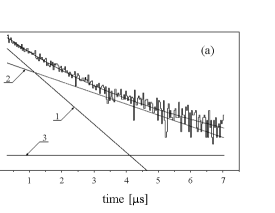
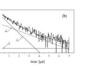
Figure 5: Time distributions of Si($dE-E$) events for Run I: (a) protons, (b) deuterons. The histograms represent the experimental data. The solid lines 1 and 2 are the exponential functions for Al and ${}^{3}\mathrm{He}$, whereas 3 is the accidental background coincidence.

Figure 5 displays the time distributions of Si($dE-E$) events for the experiment with pure ${}^{3}\mathrm{He}$. The time distributions are very well fitted by Eq. (28), using the values $\lambda_{\mathrm{Al}}=1.156\times 10^{6}\,\mbox{s}^{-1}$ and $\lambda_{\mathrm{He}}=0.457\times 10^{6}\,\mbox{s}^{-1}$ from Refs. Suzuki et al. (1987); Maev et al. (1996); Ackerbauer et al. (1998).

The second step is to remove the background arising from muon stops in aluminum. For this purpose, the time interval $\delta t=t_{2}-t_{1}$ is divided into two subintervals $\delta t_{A}=t_{3}-t_{1}$ and $\delta t_{B}$ = $t_{2}-t_{3}$. Therefore the proton yields $N_{p}$ which correspond to the two new intervals $\delta t_{A}$ and $\delta t_{B}$ have the form

$$N_{p}^{A} = \int\limits_{t_{1}}^{t_{3}}\frac{dN_{p}}{dt}dt$$

$$= \frac{D_{1}}{\lambda_{\mathrm{Al}}}e^{-\lambda_{\mathrm{Al}}\cdot t_{1}}(1-e^{-\lambda_{\mathrm{Al}}\cdot\delta t_{A}})$$

$$+ \frac{D_{2}}{\lambda_{\mathrm{He}}}e^{-\lambda_{\mathrm{He}}\cdot t_{1}}(1-e^{-\lambda_{\mathrm{He}}\cdot\delta t_{A}})+C\cdot\delta t_{A}$$

and

$$N_{p}^{B} = \int\limits_{t_{3}}^{t_{2}}\frac{dN_{p}}{dt}dt$$

$$= \frac{D_{1}}{\lambda_{\mathrm{Al}}}e^{-\lambda_{\mathrm{Al}}\cdot t_{3}}(1-e^{-\lambda_{\mathrm{Al}}\cdot\delta t_{B}})$$

$$+ \frac{D_{2}}{\lambda_{\mathrm{He}}}e^{-\lambda_{\mathrm{He}}\cdot t_{3}}(1-e^{-\lambda_{\mathrm{He}}\cdot\delta t_{B}})+C\cdot\delta t_{B}\,.$$

The total numbers of events $N_{p}^{A}$ and $N_{p}^{B}$, given for the two time intervals $\delta t_{A}$ and $\delta t_{B}$ are given by the two–dimensional amplitude distributions $(A_{jk})_{A}$ and $(A_{jk})_{B}$, created for each ($jk$) cell, where $j=1,\ldots,\ell$ and $k=1,\ldots,m$ are the cell indexes on the $dE$ (the energy losses in the thin Si detector) and the $E$ axes (the deposited energy in the thick Si detector), respectively.

The time intervals, $\delta t_{A}$ and $\delta t_{B}$, are chosen such that the difference between the proton or deuteron yields measured in the intervals $\delta t_{A}$ and $\delta t_{B}$ is independent of the aluminum muon capture contribution. This means that the first parts of Eqs. (IV) and (IV) are then equal, i.e.,

$$\frac{D_{1}}{\lambda_{\mathrm{Al}}}e^{-\lambda_{\mathrm{A}l}\cdot t_{3}}(1-e^{-\lambda_{\mathrm{Al}}\cdot\delta t_{B}})=\frac{D_{1}}{\lambda_{\mathrm{Al}}}e^{-\lambda_{\mathrm{Al}}\cdot t_{1}}(1-e^{-\lambda_{\mathrm{Al}}\cdot\delta t_{A}})\,.$$ (34)

If the initial $t_{1}$ and final $t_{2}$ measurement times are given, the middle time $t_{3}$ becomes

$$t_{3}=\frac{e^{-\lambda_{\mathrm{Al}}\cdot t_{1}}+e^{-\lambda_{\mathrm{Al}}\cdot t_{2}}}{\lambda_{\mathrm{Al}}}\cdot\ln{2}\,.$$ (35)

The difference between $N_{p}^{B}$ and $N_{p}^{A}$ is the total number of events in the resulting $(A_{jk})_{B-A}$ two–dimensional ($dE-E$) protons distribution. This distribution was obtained by subtracting channel by channel the content of the ($jk$) cell for the two $(A_{jk})_{A}$ and $(A_{jk})_{B}$ distributions.

The final number of protons $N_{p}^{\mathrm{final}}$ for the pure ${}^{3}\mathrm{He}$ measurement is then

$$N_{p}^{\mathrm{final}} = N_{p}^{B}-N_{p}^{A}$$

$$= \frac{N_{\mu}^{\mathrm{He}}\cdot\tilde{\varepsilon}_{p}\cdot\lambda_{\mathrm{cap}}^{p}(\Delta E_{p})\cdot F_{t}}{\lambda_{\mathrm{He}}}$$

$$+ C\cdot[\delta t_{B}-\delta t_{A}]$$

with

$$F_{t} = e^{-\lambda_{\mathrm{He}}\cdot t_{1}}(1-e^{-\lambda_{\mathrm{He}}\cdot\delta t_{A}})$$ (37)

$$+ e^{-\lambda_{\mathrm{He}}\cdot t_{3}}(1-e^{-\lambda_{\mathrm{He}}\cdot\delta t_{B}})\,,$$

whereas, for the $\mathrm{D}_{2}+{}^{3}\mathrm{He}$ mixture, it becomes

$$N_{p}^{\mathrm{final}} = N_{\mu}^{\mathrm{D/He}}\cdot\tilde{\varepsilon}_{p}\cdot\lambda_{\mathrm{cap}}^{p}(\Delta E_{p})\cdot F_{t}$$ (38)

$$+ C\cdot[\delta t_{B}-\delta t_{A}]$$

with

$$F_{t} = (\mathrm{a}_{\mathrm{He}}+\xi_{\mathrm{D}})\cdot\left.\frac{2e^{-\lambda_{\mathrm{He}}\cdot t_{3}}-e^{-\lambda_{\mathrm{He}}\cdot t_{1}}-e^{-\lambda_{\mathrm{He}}\cdot t_{2}}}{\lambda_{\mathrm{He}}}\right.$$

$$- \xi_{\mathrm{D}}\cdot\left[\frac{e^{-\lambda_{\mu\mathrm{d}}\cdot t_{3}}(1-e^{-\lambda_{\mu\mathrm{d}}\cdot\delta t_{B}})}{\lambda_{\mu\mathrm{d}}}\right.$$

$$- \left.\frac{e^{-\lambda_{\mu\mathrm{d}}\cdot t_{1}}(1-e^{-\lambda_{\mu\mathrm{d}}\cdot\delta t_{A}})}{\lambda_{\mu\mathrm{d}}}\right]\,.$$

Analyzing the data according to Eqs. (34) and (35) we obtained the intervals $\Delta t_{A}=[t_{1};t_{3}]=[0.51;1.098]\,\mu\mbox{s}$ and $\Delta t_{B}=[t_{3};t_{2}]=[1.098;6.0]\,\mu\mbox{s}$. The corresponding capture events in aluminum amount to $\sim 23$% of the total events. As an example, Table 2 show the number of events measured in Run II in both time intervals and both elements.

Table 2: Number of aluminum and helium events in Run II, as a function of the time intervals $\Delta t_{A}$ and $\Delta t_{B}$.

Particle	Interval $\Delta t_{A}$		Interval $\Delta t_{B}$
	Aluminum	Helium	Aluminum	Helium
Proton	2700	3600	2700	10 800
Deuteron	1150	1650	1150	5800

Our subtraction method, while reducing the number of events in helium by a factor 2 (see Table 2), yields essentially background–free events. However, Eqs. (IV) and  (38) still contain some parameters that need to be determined, namely the energy interval $\Delta E_{p}$ and the accidental coincidence background described by the constant $C$.

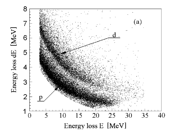
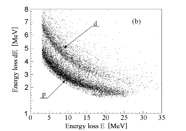
Figure 6: Two–dimensional energy distributions of the Si($dE-E$) detector events for the time interval $0.5\leq t\leq 6.0$ $\mu$s relative to the muon stop. (a) represents Run I (pure ${}^{3}\mathrm{He}$) and (b) Run II ($\mathrm{D}_{2}+{}^{3}\mathrm{He}$ mixture). The distinction between protons and deuterons is clearly visible for both measurements.

The energy intervals for detecting protons and deuterons by the Si($dE-E$) detectors were chosen such that the real detection sensitivity is the same for any initial energies. This allows us to remove any possible distortion in our amplitude distribution, which would occur for too low or too high energies. The chosen limits are $4-23$ MeV for both protons and deuterons in the thick $E$ detector. The thin $dE$ detector has two different energy intervals, namely $1-6$ MeV for the protons and $2-8$ MeV for the deuterons.

Figure 6 displays the two–dimensional ($dE-E$) distributions of events detected by the Si($dE-E$) detectors in Run I with pure ${}^{3}\mathrm{He}$ and in Run II with the $\mathrm{D}_{2}+{}^{3}\mathrm{He}$ mixture. The two distinct branches of events corresponding to the protons and the deuterons are clearly visible and lie inside our chosen energy intervals. Note that the shapes of the two–dimensional ($dE-E$) distributions obtained in the runs with pure ${}^{3}\mathrm{He}$ and with the $\mathrm{D}_{2}+{}^{3}\mathrm{He}$ mixture coincide. This indicates that there are no neglected systematic errors, and that the algorithm used for the data analysis is correct.

As to the accidental coincidence background described by the constant $C$, its contribution to Eqs. (IV) and (38) is small when compared to the muon stop contributions in Al and ${}^{3}\mathrm{He}$, as can be seen in Fig. 5. The constant $C$ was quantitatively determined in each Run by fitting the time distribution, as given in Fig. 5, including the time interval $-0.4\,\mu\mbox{s}\leq t\leq 0$ with respect to the muon stop. Details of such a fit shown in the muon decay electron time spectra are in Fig. 3.

As mentioned in the introduction, we want to determine different characteristics of the muon capture by ${}^{3}\mathrm{He}$ nuclei, namely:

• the initial energy distributions of protons and deuterons ($S(E_{p}),\ S(E_{d})$),

• the muon capture rates as function of the energy for both the protons and deuterons ($\lambda_{\mathrm{cap}}^{p}(\Delta E_{p})$ and $\lambda_{\mathrm{cap}}^{d}(\Delta E_{d})$),

• their derivatives $d\lambda_{\mathrm{cap}}^{p}/dE_{p}$ and $d\lambda_{\mathrm{cap}}^{d}/dE_{d}$.

For this purpose, following Eqs. (12), (27), and (13), we need to determine the number of protons $N_{p}(\Delta E_{p}$, $\Delta T)$ and deuterons $N_{d}(\Delta E_{d}$, $\Delta T)$ for each energy interval $\Delta E_{p}$ and $\Delta E_{d}$. In the next two subsections we describe the two approaches to determine the respective number of protons and deuterons, based on the analysis of the two–dimensional $(A_{jk})_{B-A}$ distributions as function of $dE$ and $E$ for each of the three Runs (I–III).

IV.1 Method I: Least–squares

The principle of this method is to use Monte Carlo (MC) simulations to reproduce the experimental data and to minimize the free parameters which are required by such a simulation. The simulation conditions and parameters will be given below. The energy spectra of the protons and deuterons produced by reactions (1) and (2) are divided into $i$ subintervals of 1 MeV fixed widths. Since the theoretical maximum energies are $\approx 53$ MeV for the protons and $\approx 33$ MeV for the deuterons, the numbers of subintervals are 53 and 33, respectively.

Using the experimental muon stop distribution in our target, we simulate the probability $P^{\mathrm{MC}}(A_{jk}/E_{p}^{i})$ that a proton (analogously a deuteron) produced with an energy $E_{p}^{i}$ (in the $i$-th interval $\Delta E_{p}^{i}$) will be detected by the Si($dE-E$) detectors in the ($jk$) cell of the two–dimensional distribution $A_{jk}$. This probability is

$$P^{\mathrm{MC}}(A_{jk}/E_{p}^{i})=\frac{(n_{jk})_{i}^{\mathrm{MC}}}{(n_{o})_{i}},$$ (40)

where $(n_{jk})_{i}^{\mathrm{MC}}$ is the number of simulated events detected in the ($jk$) cell when the number of protons, which were created with an initial energy $E_{p}^{i}$ from the interval $\Delta E_{p}^{i}$, is $(N_{o})_{i}$. The ($jk$) cell size is chosen arbitrarily and mainly depends on the statistics of events $(n_{jk})_{i}^{\mathrm{MC}}$ belonging to a particular cell ($jk$).

Then the MC simulated “pseudo–experimental” (i.e., normalized to the experimental counts $N_{p}^{\mathrm{final}}=N_{p}(\Delta E_{p},\Delta T)$) event numbers $(N_{jk})^{\mathrm{MC}}$ for each ($jk$) cell, become

$$(N_{jk})^{\mathrm{MC}} = N_{p}^{\mathrm{final}}\sum\limits_{i}P^{MC}(A_{jk}/E^{i}_{p})$$ (41)

$$\times \int\limits_{E^{i}_{p}}^{E^{i}_{p}+\delta E^{i}_{p}}S(E_{p})dE_{p}\,,$$

where $S(E_{p})$ is the initial proton energy distribution normalized to unity in the full energy interval $\Delta E_{p}$.

In our energy intervals $10\leq E_{p}\leq 49$ MeV and $13\leq E_{d}\leq 31$ MeV both the proton and deuteron energy distributions, $S(E_{p})$ and $S(E_{d})$, obtained via the impulse approximation model and the realistic wave functions for the ${}^{3}\mathrm{He}$ nucleus ground state Philips et al. (1975); Glöckle et al. (1990); Skibinski et al. (1999); Glöckle et al. (1996) can be well described by the expression

$$S(E_{p})=A_{p}e^{-\alpha_{p}E_{p}},$$ (42)

where the amplitude $A_{p}$ and the fall–off yield $\alpha_{p}$ are the variable parameters. Thus Eq. (41) can be rewritten as

$$(N{jk})^{MC}=N_{p}^{\mathrm{final}}\sum\limits_{i}P^{MC}(A_{jk}/E^{i}_{p})\cdot\tilde{S}(E_{p}^{i})\,,$$ (43)

where

$$\tilde{S}(E_{p}^{i})=\frac{1-e^{-\alpha_{p}\cdot\delta E_{p}^{i}}}{\alpha_{p}}S(E_{p}^{i})\,.$$ (44)

We created $(N_{jk})^{MC}$ for different values of the amplitude $A_{p}$ and the fall–off yield $\alpha_{p}$ and used the $\chi^{2}$ minimization procedure between the MC and experimental events,

$$\chi^{2}=\sum\limits_{j=1}^{l}{\sum\limits_{k=1}^{m}{\frac{\left[({N_{jk})^{\exp}-(N_{jk})^{\mathrm{MC}}}\right]^{2}}{\sigma_{N_{jk}^{\exp}}^{2}}}},$$ (45)

to obtain the best values for the parameters $A_{p}$ and $\alpha_{p}$ which describe the initial energy distribution of protons $S(E_{p})$. $(N_{jk})^{\exp}$ is the number of measured events belonging to the ($jk$) cell, obtained for pure ${}^{3}\mathrm{He}$ and the $\mathrm{D}_{2}+{}^{3}\mathrm{He}$ mixture, respectively. The $N_{p}^{\mathrm{final}}$ values of Eqs. (IV) and (38) represent the sum of the $(N_{jk})^{\exp}$ over $j$ and $k$.

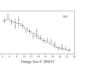
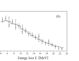
Figure 7: $E$ axis projections of the two–dimensional ($dE-E$) distributions for the protons (a) and the deuterons (b) obtained in Run II with the $\mathrm{D}_{2}+{}^{3}\mathrm{He}$ mixture. The histogram shows the experimental data, whereas the black triangles are MC events from Method I.

A second and parallel minimization is done when projecting the experimental and MC events onto the two energy axes $j$ and $k$. When projecting onto the $E$ axis, we have the experimental data as

$$(N_{k})^{\exp}=\sum\limits_{j=1}^{l}{(N_{jk})^{\exp}},$$ (46)

and the MC events as

$$(N_{k})^{\mathrm{MC}} = \sum\limits_{j=1}^{l}{(N_{jk})^{\mathrm{MC}}}$$

$$= N_{p}^{\mathrm{final}}\sum\limits_{i}{\sum\limits_{j=1}^{l}{P^{MC}(A_{jk}/}}E_{p}^{i})\cdot\tilde{S}(E^{i}_{p})\,.$$

Therefore $\chi^{2}$ becomes

$$\chi^{2}=\sum\limits_{k=1}^{m}{\frac{\left[{(N_{k})^{\exp}-(N_{k})^{\mathrm{MC}}}\right]^{2}}{\sigma_{N_{k}^{\exp}}^{2}}}\,.$$ (48)

Similar equations can be written for the second axis $j$ when we project the events onto the $dE$ axis.

Figure 7 displays the least–squares comparison of the $E$ axis projection of the two–dimensional experimental and the MC simulated distributions for the protons and the deuterons of Run II. As seen, the MC distributions correspond very well to the experimental proton and deuteron energy distributions, thus strongly supporting our analysis method I.

The amplitude and fall–off yield results from the three experimental Runs (I–III) are

$${A}_{p}= (0.832 \pm\,\,0.043)\,\,\mbox{MeV}^{-1}$$

$$\alpha_{p}= (-0.163 \pm\,\,0.002)\,\,\mbox{MeV}^{-1}$$ (49)

for the protons and

$${A}_{d}= (5.59 \pm\,\,1.39)\,\,\mbox{MeV}^{-1}$$

$$\alpha_{d}= (-0.243 \pm\,\,0.012)\,\,\mbox{MeV}^{-1}$$ (50)

for the deuterons.

Table 3: Mean proton energy distribution normalized to unity in the energy range $10\leq\mathrm{E}_{p}\leq 49$ MeV, from methods I and II.

$E_{p}$	$<S(E_{p})>$ [MeV-1]
[MeV]	Method I	Method II
10.5	0.150 (13)	0.1570 (83)
11.5	0.127 (12)	0.1309 (48)
12.5	0.108 (10)	0.1077 (35)
13.5	0.0922 (88)	0.0958 (29)
14.5	0.0784 (77)	0.0765 (24)
15.5	0.0667 (67)	0.0644 (22)
16.5	0.0568 (59)	0.0525 (22)
17.5	0.0483 (51)	0.0485 (20)
18.5	0.0411 (45)	0.0392 (18)
19.5	0.0349 (39)	0.0313 (17)
20.5	0.0297 (34)	0.0284 (16)
21.5	0.0252 (30)	0.0251 (14)
22.5	0.0215 (26)	0.0208 (14)
23.5	0.0183 (22)	0.0184 (13)
24.5	0.0155 (20)	0.0162 (11)
25.5	0.0132 (17)	0.0150 (12)
26.5	0.0112 (15)	0.01135 (28)
27.5	0.0095 (13)	0.00934 (19)
28.5	0.0081 (11)	0.00793 (16)
29.5	0.00688 (98)	0.00679 (14)
30.5	0.00585 (85)	0.00585 (22)
31.5	0.00497 (74)	0.00528 (27)
32.5	0.00422 (64)	0.00440 (21)
33.5	0.00359 (56)	0.00379 (16)
34.5	0.00305 (49)	0.00316 (13)
35.5	0.00259 (42)	0.00255 (11)
36.5	0.00220 (37)	0.00210 (9)
37.5	0.00187 (32)	0.00177 (7)
38.5	0.00158 (28)	0.00142 (6)
39.5	0.00135 (24)	0.00119 (5)
40.5	0.00114 (21)	0.00105 (4)
41.5	0.00097 (18)	0.00092 (4)
42.5	0.00082 (16)	0.00079 (3)
43.5	0.00070 (13)	0.00067 (3)
44.5	0.00059 (12)	0.00057 (2)
45.5	0.00050 (10)	0.00048 (2)
46.5	0.00043 (9)	0.00041 (2)
47.5	0.00036 (8)	0.00034 (1)
48.5	0.00031 (7)	0.00029 (1)

The capture rates $\lambda_{\mathrm{cap}}^{p}(\Delta E_{p})$ are obtained after using Eq. (43) to calculate the proton yield $N_{p}(\Delta E_{p},\Delta T)$ and then applying Eqs. (12) and (27). The differential capture rates $d\lambda^{p}_{\mathrm{cap}}/dE_{p}$ also follow from the proton yield and Eq. (13); they are given in Figs. 12 and 13 for the protons and deuterons, respectively.

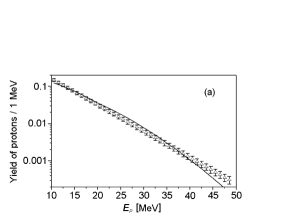
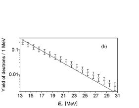
Figure 8: Experimental energy distributions (open triangles) of protons (a) and deuterons (b) found by the method I and averaged over Runs (I–III) in comparison with the theoretical model Philips et al. (1975) (solid line).

The average energy distributions $<S(E_{p}>$ and $<S(E_{d})>$ from Runs (I–III) normalized to unity for the energy intervals $10\leq E_{p}\leq 49$ MeV and $13\leq E_{d}\leq 31$ MeV are given in Table 3 for the protons and in Table 4 for the deuterons. Figure 8 displays the energy distributions $<S(E_{p})>$ and $<S(E_{d})>$ averaged over Runs (I–III) in comparison with the model distributions obtained when treating the muon capture in the simple plane–wave impulse approximation Philips et al. (1975) and in the impulse approximation with the realistic Bonn B potential Machleidt (1989) of NN interaction in the final state Skibinski et al. (1999).

Table 4: Mean deuteron energy distribution normalized to unity in the energy range $13\leq E_{d}\leq 31$ MeV, from methods I and II.

$E_{d}$	$<S(E_{d})>$ [MeV-1]
[MeV]	Method I	Method II
13.5	0.210 (44)	0.216 (11)
14.5	0.167 (36)	0.1690 (65)
15.5	0.133 (29)	0.1281 (47)
16.5	0.106 (24)	0.1043 (41)
17.5	0.084 (19)	0.0842 (35)
18.5	0.067 (16)	0.0674 (29)
19.5	0.053 (13)	0.0521 (25)
20.5	0.042 (10)	0.0426 (23)
21.5	0.0328 (84)	0.0345 (23)
22.5	0.0258 (68)	0.0251 (21)
23.5	0.0202 (55)	0.0181 (18)
24.5	0.0158 (44)	0.0132 (18)
25.5	0.0124 (35)	0.0124 (17)
26.5	0.0096 (28)	0.0101 (16)
27.5	0.0075 (23)	0.0071 (16)
28.5	0.0058 (18)	0.0058 (19)
29.5	0.0045 (14)	0.0052 (18)
30.5	0.0034 (12)	0.0044 (14)

Experimental and theoretical results agree quite well within the statistical errors for the energy ranges $10\leq E_{p}\leq 40$ MeV and $13\leq$ $E_{d}\leq 24$ MeV, respectively. For proton energies $E_{p}>40$ MeV and deuteron energies $E_{d}>24$ MeV a discrepancy exceeding the tolerable range determined by the statistical errors is observed. The cause of the discrepancy is not clear yet. It may be due to the necessity of taking into account exchange current contributions in the interaction and nucleon pair correlations in muon capture by the ${}^{3}\mathrm{He}$ nucleus.

IV.2 Method II: Bayes theorem

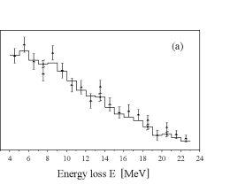
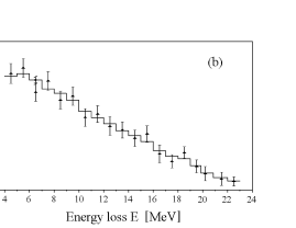
Figure 9: $E$ axis projections of the two-dimensional ($dE-E$) distributions for the protons (a) and deuterons (b) obtained in Run II. The histogram shows the experimental data, whereas the black triangles are MC events from Method II.

In this approach we use the Bayes theorem Gnedenko (1961); Johnson and Leone (1964); Box and Tiao (1992); D’Agostino (1995, 1999) to determine the initial energy distribution, $S(E)$, of the protons and the deuterons produced by muon capture in ${}^{3}\mathrm{He}$. For this purpose, we apply inverse transformations from the detected two dimensional ($dE-E$) amplitude distributions.

The relation between the probability $P(A_{jk}/E_{p}^{i})$ that a proton produced with an initial energy $E_{p}^{i}$ (in the $i$–th interval of 1 MeV width in our case) will be detected by the Si($dE-E$) telescopes and the inverse probability $P(E_{p}^{i}/A_{jk})$ (probability that a proton detected in the ($jk$) cell comes from the $\Delta E^{i}_{p}$ subinterval) is

$$P(E_{p}^{i}/A_{jk})=\frac{\tilde{S}(E^{i}_{p})\cdot P(A_{jk}/E_{p}^{i})}{\sum\limits_{i}\tilde{S}(E^{i}_{p})\cdot P(A_{jk}/E_{p}^{i})}\,.$$ (51)

The probability $P(A_{jk}/E_{p}^{i})$ is given by the MC simulated probability $P^{MC}(A_{jk}/E_{p}^{i})$ defined in Eq. (40).

In the first step of the analysis we start from the initial energy distribution $S_{o}(E_{p})=S(E_{p})$ given by (42) with an arbitrary set of parameters. When using the probability given by Eq. (51) and the experimental data of each ($jk$) cell, we obtain a set of $i$ relations

$$N_{p}(\Delta E_{p},\Delta T)\cdot\tilde{S}(E_{p}^{i})=\frac{\sum\limits_{j=1}^{l}{\sum\limits_{k=1}^{m}{P(E_{p}^{i}/A_{jk})}\cdot(N_{jk})^{\exp}}}{P(A/E_{p}^{i})}\,,$$ (52)

where $N_{p}(\Delta E_{p},\Delta T)$ corresponds to Eqs. (10) or (26), and $P(A/E_{p}^{i})$ is the probability that a proton of initial energy $E_{p}^{i}$ is detected anywhere in the proton branch of the two–dimensional distribution $A_{jk}$. This probability can be written as

$$P(A/E_{p}^{i})=\sum\limits_{j=1}^{l}{\sum\limits_{k=1}^{m}{P^{MC}(A_{jk}/E_{p}^{i})}}\,.$$ (53)

We then compare $N_{p}(\Delta E_{p},\Delta T)$ and the experimental counts $N^{\exp}=\sum\sum(N_{jk})^{\exp}$ for each $i$-th interval via a $\chi^{2}$ analysis and obtain a proton energy distribution $S(E_{p}^{i})$ from Eqs. (52) and (44). As long as the $\chi^{2}$ is not satisfactory, we re–use the last $\tilde{S}(E_{p}^{i})$ as the starting values in Eq. (51) in the next iteration.

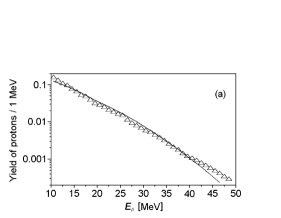
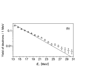
Figure 10: Experimental energy distributions (open triangles) of protons (a) and deuterons (b) found by the method II and averaged over Runs (I–III) in comparison with the theoretical model Philips et al. (1975) (solid line).

In addition, the initial energy distributions of the protons and deuterons can also be derived by analyzing the projections of the two–dimensional distribution $(A_{jk})$ onto the $dE$ axis $(A_{j})$ and the $E$ axis $(A_{k})$. The equations for the $dE$ axis are

$$P(E_{p}^{i}/A_{j})=\frac{\tilde{S}(E_{p}^{i})\sum\limits_{k=1}^{m}{P^{MC}(A_{jk}/E_{p}^{i})}}{\sum\limits_{i}{\tilde{S}(E_{p}^{i})\cdot\sum\limits_{k=1}^{m}{P^{MC}(A_{jk}/E_{p}^{i})}}}$$ (54)

and

$$N_{p}(\Delta E_{p},\Delta T)\cdot\tilde{S}(E_{p}^{i})=\frac{\sum\limits_{j=1}^{l}{P(E_{p}^{i}/A_{j})\cdot(N_{j})^{\exp}}}{P(A/E_{p}^{i})}\,.$$ (55)

Similar equations can be written for the $E$ axis. Using the above equations, we obtain simulated values for the proton and deuteron yields as measured by the Si($dE-E$) detectors. Figure 9 shows the projections of the experimental and simulated ($dE-E$) distributions for protons and deuterons onto the $E$ axis.

The mean proton $<S(E_{p})>$ and deuteron $<S(E_{d})>$ energy distributions from Runs (I–III) are given in Tables 3 and 4. The mean values are also displayed in Fig. 10. It is important to note that the distribution $S(E_{p})$ does practically not depend on the form of the energy distribution $S_{o}(E_{p})$ which is chosen for the first iteration. Variation errors in the determination of $S(E_{p})$ fall within the statistical errors of $(N_{jk})^{\exp}$. Since Eqs. (52) and (55) (as well as the other projection) have an identical solution, their comparison makes it possible to conclude, with an accuracy determined by the statistics of the detected events, that there are no systematic errors in the analysis of experimental data.

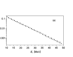
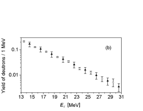
Figure 11: Comparison of the proton (a) and deuteron (b) energy distributions found by methods I (black triangles) and II (open circles) averaged over Runs (I–III). For sake of visibility, we plotted both methods results alternatively.

A comparison between the experimental energy distributions given in Fig. 10 and the energy distribution calculated by the impulse approximation reveals some discrepancies of the same character as in the method I analysis, as long as the interactions between the reaction products (1) and (2) are considered and a realistic Bonn B Skibinski et al. (1999) nucleon-nucleon potential is employed.

The capture rates $\lambda_{\mathrm{cap}}^{p}(\Delta E_{p})$ as well as the differential capture rates $d\lambda^{p}_{\mathrm{cap}}/dE_{p}$ which are found from Eqs. (52) and (55) using Eqs. (12), (13), and (27) are given in Fig. 12 for the protons and in Fig. 13 for the deuterons.

V Conclusions

Table 5: Relations $d\lambda_{\mathrm{cap}}^{p}(E_{p})/dE_{p}$ found by methods I and II and averaged over Runs (I–III). The proton energies $E_{p}$ correspond to the middle of the respective 1 MeV intervals.

$E_{p}$	$<\frac{d\lambda_{\mathrm{cap}}^{p}}{dE_{p}}>$ [MeV-1s-1]
[MeV]	Method I	Method II
10.5	5.49 (59)	5.77 (47)
11.5	4.67 (51)	4.81 (35)
12.5	3.98 (44)	3.95 (28)
13.5	3.38 (38)	3.52 (25)
14.5	2.88 (33)	2.81 (20)
15.5	2.45 (29)	2.37 (17)
16.5	2.08 (25)	1.93 (15)
17.5	1.77 (22)	1.78 (13)
18.5	1.51 (19)	1.44 (11)
19.5	1.28 (16)	1.151 (95)
20.5	1.09 (14)	1.041 (88)
21.5	0.93 (12)	0.920 (77)
22.5	0.79 (11)	0.763 (71)
23.5	0.671 (92)	0.675 (64)
24.5	0.570 (80)	0.595 (56)
25.5	0.485 (69)	0.549 (55)
26.5	0.412 (60)	0.417 (28)
27.5	0.350 (52)	0.343 (23)
28.5	0.298 (45)	0.291 (19)
29.5	0.253 (39)	0.249 (17)
30.5	0.215 (34)	0.215 (16)
31.5	0.183 (29)	0.194 (16)
32.5	0.155 (26)	0.162 (13)
33.5	0.132 (22)	0.139 (11)
34.5	0.112 (19)	0.116 (9)
35.5	0.095 (17)	0.094 (7)
36.5	0.081 (14)	0.077 (6)
37.5	0.069 (12)	0.065 (5)
38.5	0.058 (11)	0.052 (4)
39.5	0.050 (9)	0.044 (3)
40.5	0.042 (8)	0.038 (3)
41.5	0.036 (7)	0.034 (3)
42.5	0.030 (6)	0.029 (2)
43.5	0.026 (5)	0.024 (2)
44.5	0.022 (4)	0.021 (2)
45.5	0.019 (4)	0.018 (1)
46.5	0.016 (3)	0.015 (1)
47.5	0.013 (3)	0.013 (1)
48.5	0.011 (2)	0.011 (1)

Table 6: Relations $d\lambda_{\mathrm{cap}}^{d}(E_{d})/dE_{d}$ found by methods I and II and averaged over Runs (I–III). The deuteron energies $E_{d}$ correspond to the middle of the respective 1 MeV intervals.

$E_{d}$	$<\frac{d\lambda_{\mathrm{cap}}^{d}}{dE_{d}}>$ [MeV-1s-1]
[MeV]	Method I	Method II
13.5	4.46 (94)	4.74 (36)
14.5	3.56 (77)	3.70 (26)
15.5	2.84 (63)	2.81 (19)
16.5	2.26 (51)	2.29 (16)
17.5	1.80 (42)	1.84 (13)
18.5	1.43 (34)	1.48 (11)
19.5	1.13 (28)	1.141 (87)
20.5	0.90 (22)	0.933 (74)
21.5	0.70 (18)	0.756 (67)
22.5	0.55 (15)	0.550 (55)
23.5	0.43 (12)	0.397 (47)
24.5	0.340 (95)	0.289 (44)
25.5	0.266 (76)	0.272 (41)
26.5	0.207 (61)	0.221 (37)
27.5	0.161 (49)	0.156 (35)
28.5	0.124 (39)	0.127 (42)
29.5	0.096 (31)	0.114 (41)
30.5	0.074 (25)	0.095 (31)

The proton and deuteron energy distributions found by methods I and II largely coincide within the measurement errors, which points to the compatibility of the different approaches and to the absence of any systematic errors which may have been neglected in the analysis of the experimental data (see Fig. 11). However, the errors on $S(E_{p})$ and $S(E_{d})$ found by both methods are different. The analysis using method II gives a more precise information about the proton and deuteron energy distributions than method I. In method I, we compare using the numbers of detected events from a ($jk$) cell with similar MC simulated data. Such numbers are the sums of the contributions from all $i$-th proton energy subintervals $\Delta E^{i}_{p}$. In method II, we have much deeper relations because the comparisons are performed via Eq. (52) for each $i$–th subinterval separately and all comparisons should be simultaneously satisfactory.

Similar remarks hold for the differential capture rates $d\lambda_{\mathrm{cap}}^{p}(E_{p})/dE_{p}$ and $\lambda_{\mathrm{cap}}^{p}(\Delta E_{p})$, as seen in Fig. 12. Tables 5 and 6 list the values of $<d\lambda_{\mathrm{cap}}^{p}(E_{p})/dE_{p}>$ and $<d\lambda_{\mathrm{cap}}^{d}(E_{d})/dE_{d}>$ found from the analysis of the Runs (I–III) with pure ${}^{3}\mathrm{He}$ and $\mathrm{D}_{2}+{}^{3}\mathrm{He}$ mixtures data by methods I and II.

Table 7: Muon capture rates by ${}^{3}\mathrm{He}$ nucleus (in s^-1) followed by the proton and deuteron production following methods I and II.

Method	I	II
$\lambda_{\mathrm{cap}}^{p}(10\leq E_{p}\leq 49\,\mbox{MeV})$	$36.7\pm 1.2$	$36.8\pm 0.8$
$\lambda_{\mathrm{cap}}^{d}(13\leq E_{p}\leq 31\,\mbox{MeV})$	$21.3\pm 1.6$	$21.9\pm 0.6$

The addition of the differential rates in Tables 5 and 6 yields the muon capture rates by the ${}^{3}\mathrm{He}$ nucleus followed by proton and deuteron production in the final state in the energy intervals $10\leq\mathrm{E}_{p}\leq 49$ MeV and $13\leq E_{d}\leq 31$ MeV, respectively (see Table 7).

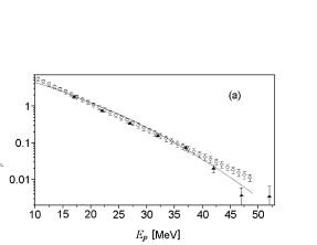
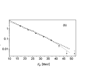
Figure 12: Differential rates $d\lambda_{\mathrm{cap}}^{p}(E_{p})/dE_{p}$ (open circles) found by methods I (a) and II (b) averaged over Runs (I–III). Black triangles are the results of Refs. Kuhn et al. (1994); Cummings et al. (1992); the solid line corresponds to the model Philips et al. (1975).

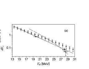
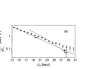
Figure 13: Differential rates $d\lambda_{\mathrm{cap}}^{d}(E_{d})/dE_{d}$ (black triangles) found by methods I (a) and II (b) and averaged over Runs (I–III). Black boxes are the results of Refs. Kuhn et al. (1994); Cummings et al. (1992); the solid line corresponds to the model Philips et al. (1975); the dotted line is based on calculations from Ref. Skibinski et al. (1999).

Looking more closely at Figs. 12 and 13, our results and their comparison with the experimental data Kuhn et al. (1994); Cummings et al. (1992) and the calculations Philips et al. (1975); Skibinski et al. (1999); Glöckle et al. (1996) indicate the following results for the protons and deuterons. Experimental (obtained by methods I and II) and calculated differential rates $d\lambda_{\mathrm{cap}}^{p}(E_{p})/dE_{p}$ and $\lambda_{\mathrm{cap}}^{p}(\Delta E_{p})$ for muon capture by the ${}^{3}\mathrm{He}$ nucleus followed by proton production in the energy range $10\leq E_{p}\leq 40$ MeV show quite good agreement both in form and in magnitude. The calculations were carried out in the simple plane–wave impulse approximation (PWIA) with allowance made for final–state interaction of reaction (1) and (2) products. However, there is a difference between the results of the present paper and the calculations Philips et al. (1975) for proton energies $E_{p}>40$ MeV.

The measured dependence $d\lambda_{\mathrm{cap}}^{d}(E_{d})/dE_{d}$ found by using methods I and II is quite well described by the theoretical PWIA dependence Philips et al. (1975) in the deuteron energy ranges $13\leq E_{d}\leq 20$ MeV (Method I) and $13\leq E_{d}\leq 17$ MeV (Method II), respectively. For deuteron energies $E_{d}>20$ MeV there is a noticeable discrepancy between experiment and theory Philips et al. (1975). The measured values of $d\lambda_{\mathrm{cap}}^{d}(E_{d})/dE_{d}$ and the PWIA calculations Skibinski et al. (1999) with the refined realistic NN interaction potential (Bonn B) appreciably disagree over the entire deuteron energy range.

Next, we can estimate the total capture rate (full energy range $[0;\infty)$) using a simple extrapolation of our data at low energies and a one–exponential weighted fit of the differential capture rate in the full energy range. Using the function

$$\frac{d\lambda_{\mathrm{cap}}^{p}(E_{p})}{dE_{p}}=H\cdot e^{-G\cdot E_{p}}\,,$$ (56)

where $H$ and $G$ are free parameters, we obtain the total capture rate for the proton as their ratio

$$\lambda_{\mathrm{cap}}^{p}=\frac{H}{G}\,.$$ (57)

Results for protons and deuterons, using both methods, are given in Table 8. The summed rate $\lambda_{\mathrm{cap}}^{p}+\lambda_{\mathrm{cap}}^{d}$ (which corresponds to Eq. (7) without the triton contribution) is also compared to other experimental Zaĭmidoroga et al. (1963); Auerbach et al. (1965); Maev et al. (1996) and theoretical Yano (1964); Philips et al. (1975); Congleton (1994) values. Agreement between our results and previous ones is excellent.

Table 8: Total muon capture rate for reactions (1) and (2). The results of this work is an estimation from both methods I (least–square) and II (Bayes theorem).

Method	$\lambda_{\mathrm{cap}}^{p}$	$\lambda_{\mathrm{cap}}^{d}$	$\lambda_{\mathrm{cap}}^{p}+\lambda_{\mathrm{cap}}^{d}$
	[s-1]	[s-1]	[s-1]
This work
Least–square	$187\pm 11$	$491\pm 125$	$678\pm 126$
Bayes	$190\pm 7$	$497\pm 57$	$687\pm 60$
Zaimidoroga Zaĭmidoroga et al. (1963)			$660\pm 160$
Auerbach Auerbach et al. (1965)			$665\>\>^{+\>170}_{-\>430}$
Maev Maev et al. (1996)			$720\pm 70$
Yano Yano (1964)			670
Philips Philips et al. (1975)	209	414	623
Congleton Congleton (1994)			650

An experimental determination of muon capture on ${}^{3}\mathrm{He}$ nuclei makes a study of electromagnetic and weak interactions of elementary particles with 3N systems possible without introducing uncertainties due to inadequate approximations of 3N states in the analysis. According to the theory, meson exchange currents must also be taken into account in future analysis of experimental data. As compared with Refs. Kuhn et al. (1994); Cummings et al. (1992), this experiment yields for the first time information on the “softer” region of proton and deuteron energy spectra, which is more sensitive to the theoretical models describing the final–state nucleon–nucleon interactions.

Finally it should be mentioned that by increasing the efficiencies of the proton and deuteron detection systems and their functional capabilities, by decreasing the lower and increasing the upper thresholds in the Si($dE-E$) telescopes, the above method will provide precise information on the characteristics of muon capture by bound few–nucleon systems. It then becomes possible to verify various theoretical models of muon capture by helium nuclei and to clarify the nature of discrepancies between the results of the present paper and the experimental data Kuhn et al. (1994); Cummings et al. (1992).