One-neutron removal reactions on light neutron-rich nuclei

Abstract

A study of high energy (43–68 MeV/nucleon) one-neutron removal reactions on a range of neutron-rich psd-shell nuclei (Z = 5–9, A = 12–25) has been undertaken. The inclusive longitudinal and transverse momentum distributions for the core fragments, together with the cross sections have been measured for breakup on a carbon target. Momentum distributions for reactions on tantalum were also measured for a subset of nuclei. An extended version of the Glauber model incorporating second order noneikonal corrections to the JLM parametrisation of the optical potential has been used to describe the nuclear breakup, whilst the Coulomb dissociation is treated within first order perturbation theory. The projectile structure has been taken into account via shell model calculations employing the psd-interaction of Warburton and Brown. Both the longitudinal and transverse momentum distributions, together with the integrated cross sections were well reproduced by these calculations and spin-parity assignments are thus proposed for ¹⁵B, ¹⁷C, ^19-21N, ^21,23O, ^23-25F. In addition to the large spectroscopic amplitudes for the $\nu 2$s_1/2 intruder configuration in the $N=9$ isotones,¹⁴B and ¹⁵C, significant $\nu 2$s${}_{1/2}^{2}$ admixtures appear to occur in the ground state of the neighbouring $N=10$ nuclei ¹⁵B and ¹⁶C. Similarly, crossing the N=14 subshell, the occupation of the $\nu 2$s_1/2 orbital is observed for ²³O, ^24,25F. Analysis of the longitudinal and transverse momentum distributions reveals that both carry spectroscopic information, often of a complementary nature. The general utility of high energy nucleon removal reactions as a spectroscopic tool is also examined.

PACS number(s): 24.10.-i, 25.60.-t, 25.60.Dz, 25.60.Gc

I Introduction

High energy heavy-ion projectile fragmentation has been investigated now for some 25 years [1, 2]. The initial emphasis centred on reactions employing stable beams at relativistic energies [3, 4] and the observed momentum distributions (typically Gaussian in form with FWHM $\sim$ 200 MeV/$c$) were interpreted within a statistical description as reflecting the Fermi momentum of the removed nucleons [5]. Further refinements lead to more sophisticated models incorporating the peripheral nature of the reaction process [6, 7]. Beyond relatively simple considerations, such as the surface cluster model [7], the projectile structure played no role in the fragment distributions.

More recently, the investigation of fragmentation reactions using radioactive beams has lead to the recognition of narrow fragment momentum distributions (FWHM $\sim$ 50 MeV/$c$) as a signature of the extended valence nucleon density distributions in halo nuclei [8]. Originally these momentum distributions were assumed, in terms of the transparent limit of the Serber model [9], to be a direct mapping via the Fourier transform, of the valence nucleon(s) wave function. Detailed investigation of the role played by the reaction mechanisms, particularly in the case of the single-neutron halo nucleus ¹¹Be [10, 11] demonstrated that such an interpretation was not generally applicable. The longitudinal core fragment momentum distributions have been suggested [12, 13, 14] to be less influenced by such effects and as such to represent a cleaner probe. As foreseen in the original work of Serber [9] and more explicitly in the case of heavy ions by Hüfner and Nemes [6], the requirement of core survival drives few nucleon removal to probe essentially only that part of the valence nucleon(s) wave function residing outside the core [17, 18]. Consequently, in the spirit of the spectator-core model of Hussein and McVoy [19], various Glauber-type approaches to modelling the dissociation of energetic beams of nuclei far from stability have been developed [15, 16, 17, 18, 20, 21, 22, 23, 24, 25]. The essential results are that the momentum distributions, as first recognized by Bonaccorso and Brink [26] and Sagawa and Yazaki [15], reflect the angular momentum ($l$) of the removed nucleon, whilst the corresponding cross section may provide a measure of the associated spectroscopic strength [27].

Recently, experimental measurements of single-nucleon removal reactions including $\gamma$-ray detection have demonstrated that significant population of core fragment excited states may occur [27, 28, 29, 30, 31, 32, 33, 34]. The inclusion of the core states within the theoretical framework [23, 37], as foreseen in the original work of Sagawa and Yazaki [15], has lead to the proposal that such reactions (often termed “knockout” [35]) may be used as a spectroscopic tool [23, 28]. To date, however, this approach has been largely confined to selected weakly bound halo and near dripline systems [28, 29, 30, 31, 32, 33, 36].

The objective of the present study was to undertake a systematic study of single-neutron removal reactions over a range of neutron-rich nuclei. For these purposes the light psd-shell nuclei were selected as the nuclear structure could be reliably calculated within the shell model. The region encompassed a number of nuclei of current interest and the production rates were relatively high. The use of high energy nucleon-removal reactions as a spectroscopic tool could thus be verified on a number of near stable nuclei with well known ground state structures. Additionally, the structural evolution with isospin across the psd-shell, as expressed in the core fragment observables, could be explored. As will be demonstrated, even inclusive measurements of the core fragments when executed using a broad range high acceptance spectrograph offer a means to survey changes in structure over a wide range of isospin in a single measurement.

Earlier measurements of halo nuclei have suggested that the influence of nuclear and Coulomb dissociation on the core fragment longitudinal momentum distributions is relatively weak [12, 13, 14, 38]. In order to explore further such effects, both Carbon and Tantalum targets have been used in the present work. The results obtained for the longitudinal momentum distributions and cross sections on the Carbon target have been briefly described elsewhere [39]. Here further details of the experimental techniques are given along with a detailed account of the theoretical models. In addition, the results obtained for the transverse momentum distributions using the Carbon target are presented, as are the longitudinal distributions from reactions on Tantalum.

The paper is organized as follows. The experimental setup and techniques are described in Section II and the experimental results are presented in Section III. Sections IV to VII are devoted to the description of eikonal based modelling of nuclear and Coulomb dissociation. The results and comparison to calculations are discussed in Section VIII. A discussion, in the light of the present results, of the utility of single-nucleon removal as a spectroscopic tool is presented in section IX. The paper concludes (Section X) with a summary and perspectives. Explicit analytical formulae pertaining to the Coulomb dissociation calculations are presented in Appendix A. The results of the shell model and cross section calculations are tabulated in Appendix B.

II Experimental method

The experiment was performed at the GANIL coupled cyclotron facility. The secondary beams were produced via the fragmentation of an intense ($\sim 1\mu$Ae) 70 MeV/nucleon ⁴⁰Ar¹⁷⁺ primary beam on a 490 mg/cm² thick carbon target. The reaction products were collected and analysed (B$\rho$=2.880 Tm) using the SISSI device [40] coupled to the beam analysis spectrometer. The resulting secondary beam was composed of ^12-15B, ^14-18C, ^17-21N, ^19-23O and ^22-25F nuclei with energies between 43 and 68 MeV/nucleon and intensities ranging from $\sim$600 pps (¹⁵C) to $\sim$1 pps (²⁵F). The energy spread in the beam, as defined by the acceptance of the beam analysis spectrometer, was $\Delta E/E$=1%. Secondary reaction targets of carbon (170 mg/cm²) and tantalum (190 mg/cm²) were used.

Owing to the large energy spread in the secondary beam, an energy-loss spectrometer was required to undertake a high resolution measurement of the core fragment momentum distributions [8]. In the present case, the SPEG spectrometer [41] was employed and operated at a central angle of zero degree in a dispersion matched mode for which an intrinsic resolution of $\delta p/p$=4.5$\times$10^-4 (FWHM) was achieved. The final resolution, including target effects was $\delta p/p$=3.5$\times$10^-3 (FWHM). The overall momentum acceptance of the spectrometer was 7%, which permitted the momentum distributions for the fragments resulting nuclei from one-neutron removal on all the nuclei of interest to be obtained in a single setting for each target (B$\rho_{SPEG}$=2.551 Tm for the carbon target and B$\rho_{SPEG}$=2.615 Tm for tantalum).

Importantly, the broad angular acceptances of the spectrometer — 4^∘ in the horizontal (bending) and vertical planes — provided, in the case of the carbon target, for almost complete collection (see below) of the core fragments, obviating any ambiguities in the integrated cross sections and longitudinal momentum distributions that may arise from limited transverse momentum acceptances [42, 43, 44]. In the case of the tantalum target (Section VIIC and ref. [45]), the effects of multiple scattering and Coulomb deflection resulted in greatly reduced effective transverse momentum acceptances that curtailed the extraction of any reliable transverse momentum distributions or cross sections. An investigation of the effects of incomplete transverse acceptances on the longitudinal momentum distributions is presented elsewhere [45, 46].

Ion identification at the focal plane of SPEG was achieved using the energy loss derived from a gas ionisation chamber and the time-of-flight between a thick plastic stopping detector and the cyclotron radio-frequency. Additional information was provided by the residual energy measurement furnished by the plastic detector and the time-of-flight with respect to a thin-foil microchannel plate detector located at the exit of the beam analysis spectrometer. Two large area drift chambers straddling the focal plane of SPEG were employed to determine the angles of entry of each ion and, consequently, allowed the focal plane position spectra to be reconstructed. The calibration in angle was performed using a tightly collimated beam and a calibrated mask placed at the entrance to the spectrometer. The momentum of each particle was derived from the reconstructed focal plane position. Calibration in momentum was achieved by removing the reaction target and stepping the mixed secondary beam of known rigidity along the focal plane. This procedure also facilitated a determination of the efficiency across the focal plane for the collection of the reaction products — the range of angles accepted by the spectrograph being restricted at the limits of the focal plane. Where necessary, corrections were then applied to account for any reduction in efficiency.

The angles of incidence on target of the secondary beam particles were determined using two beam tracking detectors (each comprising four 10$\times$10 cm² drift chambers) located in the analysis line of the spectrometer. The calibration in incident angle was derived from the trajectories reconstructed at the focal plane of the spectrometer for a measurement made with the target removed and the spectrometer set to the same rigidity as the analysis line. Consequently, the transverse momentum distributions for the core fragments could be reconstructed on an event-by-event basis from the incident projectile angle and the core fragment outgoing angle. The beam envelope was approximately Gaussian in form and characterized by half-angles of $\Delta\theta_{1/2}$=0.35^∘ and $\Delta\phi_{1/2}$=0.5^∘ (FWHM) in the horizontal and vertical planes respectively. Owing to the superior resolution in the determination of the angles in the bending (horizontal) plane of the spectrometer ($\delta\theta$=0.1^∘, $\delta\phi$=0.4^∘ (FWHM)), the transverse momentum distributions presented here have been reconstructed in this plane ($p_{x}$), with final resolutions including multiple scattering of some 5% being achieved.

The intensities of the various components of the secondary beam were derived from a measurement of the primary beam current, which was recorded continuously during the experiment using a non-interceptive monitor, with respect to runs taken with the secondary reaction target removed and the spectrometer set to the same rigidity as the beamline. A redundant check was also provided by counting rates in two microchannel plate detectors placed in the incident secondary beam: one, as noted above, at the exit of the beam analysis spectrometer and another located on the upstream side of the secondary reaction target. The final cross sections were determined using an average of these three normalisations and the uncertainties quoted include contributions from both the statistical uncertainty and that arising from the determination of the secondary beam intensities (typically $\sim$ 7%).

The core fragment angular distributions were inspected to ensure that no events were lost due to the finite acceptance of the spectrometer ($\Delta\Omega$=5 msr). For the reactions on the C target only in the cases of the broadest distributions did the losses exceed a few percent. The number of events not detected was estimated based on extrapolations of Gaussian adjustments to the measured angular distributions. Corrections were also applied where necessary to those nuclei falling near the limits of the focal plane (see above). The final uncertainty in the cross section includes an estimate ($\sim$ 5-10%) of the uncertainties in these two corrections. As discussed in Section VIIC, for the reactions on the Ta target extremely broad angular distributions were encountered, which precluded any reliable estimates of the transverse momentum distributions and cross sections to be made.

In many instances — most notably ¹⁴B, ^15,16C and ^17,18N — asymmetric longitudinal momentum distributions exhibiting low momentum tails were observed (Fig. 1). The origin of these events is discussed in Section VIIIA. The cross sections reported here include these events (typically $\sim$ 5%).

To compare the measured distributions with the theoretical ones, all broadening effects inherent in the measurements should be taken into account. These effects arise from the differential energy losses of the projectile and the fragment in the target, energy and angular straggling in the target and the detector and spectrometer resolutions. In addition, for the longitudinal momentum distributions the Lorentz transformation from the laboratory to projectile frame of reference must be taken into account. In order to provide an estimate of the relative importance of these effects on momentum distributions, a Monte Carlo based simulation was developed. As an example, an evaluation of the effects for two nuclei with distributions representative of those encountered here are provided in Table I. The overall effect in the case of the longitudinal distributions is some 10–13% and is dominated by the Lorentz contraction. In the case of the transverse momentum distributions, the broadening is relatively weak (at most some 5%) and is dominated by the angular resolution of the spectrometer.

The widths of the momentum distributions were derived from Gaussian adjustments to the central region ($\sim$FWHM) of each distribution, thus avoiding any bias introduced by low momentum tails. The use of other lineshapes (such as a Lorentzian), or a simple statistical analysis [14] produced essentially identical results. The widths, noted FWHM_cm in Table II, are quoted in the projectile frame and have been corrected for the various broadening effects discussed above.

III Results

The core fragment longitudinal momentum distributions measured using a carbon target are displayed in Fig. 1. In order to facilitate their comparison, each distribution is displayed over the same total momentum range of 700 MeV/$c$. The estimated widths, taking into account the various experimental effects discussed above, are shown in Fig. 2 and are listed in Table II (FWHM${}^{cm}_{pz}$). The corresponding single-neutron removal cross sections are tabulated in Table II and the evolution along the isotopic chains is presented in Fig. 3.

The transverse momentum distributions $p_{x}$ from breakup on the carbon target are presented in Fig. 4. The same total momentum range (here 600 MeV/$c$) has been used to display all the results to facilitate the comparison. The widths extracted from the measured distributions, taking into account all broadening effects (Section II), are listed in Table II (FWHM${}^{cm}_{px}$). A comparison of the widths of the longitudinal and transverse momentum distributions is provided in Fig 2. The transverse distributions are systematically somewhat broader, a feature already observed in reactions with stable beams [47]. More interestingly, the transverse distributions exhibit the same trends as the longitudinal distributions, suggesting that the sensitivity to the projectile structure expected for the latter is also present to a similar degree in the transverse distributions. As will be discussed further in Sections V-B and VIII, the transverse momentum distributions present somewhat more complex forms than the longitudinal distributions. It should be stressed that the widths quoted here are only meant to serve as a comparative guide.

For a number of nuclei (¹⁴B, ^15-17C and ^17-19N) the core fragment longitudinal momentum distributions from reactions on a Ta target were also measured (Fig. 5). The momentum widths, which are seen to be almost identical with those obtained on the C target, are listed in Table III. As outlined in Section II, the corresponding transverse momentum distributions were observed to be much broader than the acceptances of the spectrograph (see, for example, Fig. 16). As such no reliable cross sections could be derived.

As noted in Tables II and III, a number of the nuclei studied in the present work have been investigated elsewhere. In the cases of ¹⁴B and ^15,17,18C measurements made at similar energies on a Be target by Bazin et al. [48, 49] found longitudinal momentum distributions with widths in good agreement with those presented here. The associated single-neutron removal cross sections are, however, significantly smaller than those measured in the present work. As pointed out in our earlier paper [39] the origin of this discrepancy lies in the rather limited acceptances of the A1200 fragment separator. This is clearly apparent from the transverse momentum distributions presented here (Fig. 4) [45] and is also confirmed by more recent measurements of ¹⁴B [30] and ^16,17C [32] undertaken using the high acceptance S800 spectrograph (Table II).

Very recently a measurement for ¹⁶C (83 MeV/nucleon) on a C target has been reported [50]. The results, which were obtained using a new time-of-flight technique to deduce the core momentum distribution [51], are in very good agreement with those reported here.

A measurement has also been carried out with the time-of-flight technique, at an energy somewhat higher (72 MeV/nucleon) than that employed here, of the breakup of ²³O by carbon [51]. The resulting ²²O longitudinal momentum distribution is in good agreement with the present work. Moreover, as discussed in Section VIII-D, the corresponding one-neutron removal cross section (233$\pm$37 mb) is in good agreement with that calculated here (Tables II and IV).

At much higher energies ($\sim$900 MeV/nucleon), the single-neutron breakup of ¹⁷C by carbon has also been measured [38, 52]. A width (FWHM) of 141$\pm$6 MeV/$c$, slightly broader than reported here, was extracted [38] together with a cross section of 129$\pm$22 mb [52]. Recently an experiment using the same setup as that of refs. [38, 52] has been carried out to explore single-neutron removal on neutron-rich isotopes of N, O and F at some 900 MeV/nucleon. The preliminary results for the momentum distributions — in particular for ²³O (Section VIII-D) — are in very good agreement with those reported here [53].

In the case of reactions on the Tantalum target (Table III), there is a relative paucity of work with high-Z targets with which comparison can be made. Indeed, of the nuclei measured here, the literature reports results for only ¹⁴B and ^15,17C. In the case of the former, very good agreement is found with the measurement made employing the S800 spectrometer [30], whilst the earlier work of Bazin et al. found a somewhat narrower core momentum distribution [49]. The core momentum distribution measured for ¹⁵C in the same experiment [49] is in reasonable agreement with that observed here. In the case of the heavier isotope, ¹⁷C, a preliminary study [80] reported a momentum distribution consistent with that found in the present work. Unfortunately the more complete study of Maddalena and Shyam [79] does not quote any widths for the momentum distributions.

In order to examine quantitatively the relationship between the projectile structure and the measured distributions we now turn to a detailed development of the necessary reaction theory.

IV Extended Glauber model for nuclear dissociation

The ensemble of data presented in the previous section constitutes a test not only for the structure models of neutron rich nuclei in p–sd shell but also for the description of the reaction mechanisms involved. The aim of this section is to provide a model that, starting from realistic projectile wave functions and taking properly into account the reaction mechanism, can explain the momentum distributions and cross sections. In the formal development, the principle features of which are similar to approaches developed by Esbensen [18], Bertsch et al. [20, 54], Negoita et al. [22] and Tostevin [23, 37], we have attempted to retain the role played by the wave function via its Wigner transform as this reveals clearly the momentum content. The formulae obtained for the fragment momentum distributions and cross sections explicitly display, in the spirit of the Glauber model, the distorting functions arising from the reaction mechanism. The details concerning the practical calculation of some basic ingredients — in particular the S-matrix elements — are also provided.

We shall assume that the ground state of the projectile $(J^{\pi})$ could be approximated by a superposition of configurations of the form $[I_{c}^{\pi}\otimes nlj]^{J^{\pi}}$, where $I_{c}^{\pi}$ denotes the core states and $nlj$ are the quantum numbers specifying the single particle wave function of the last neutron, taken here as Woods-Saxon wave functions evaluated using the effective separation energy $S^{eff}_{n}=S_{n}+E_{ex}^{c}$ ($E_{ex}$ being the excitation energy of the core state). We neglect coupling of core states to the final state and dynamical excitation of excited core states in the reaction. In this approximation the reaction can populate a given core state only to the extent that there is a nonzero spectroscopic factor $C^{2}S(I^{\pi}_{c},nlj)$ in the projectile ground state. When more than one configuration contributes to a given core state, then the total cross section for one neutron removal is written, following refs. [23, 37], as an incoherent superposition of single particle cross sections:

$$\sigma_{-1n}(I^{\pi}_{c})=\sum_{nlj}C^{2}S(I^{\pi}_{c},nlj)\;\sigma_{sp}(nlj,S^{eff}_{n}).$$ (1)

The total inclusive one-neutron removal cross section ($\sigma_{-1n}^{Glauber}$) is then the sum over the cross sections to all core states. A similar relation holds for the momentum distributions. The coordinate system used in the calculations is sketched in Fig. 6, whereby the impact parameters for the neutron and the core are given by,

$$\vec{b}_{n}=\vec{R}_{\perp}+\frac{A_{c}}{A_{c}+1}\vec{s},$$ (2)

$$\vec{b}_{c}=\vec{R}_{\perp}-\frac{1}{A_{c}+1}\vec{s}.$$ (3)

We shall neglect recoil effects, so that ($A_{c}\gg 1$),

$$\vec{b}_{n}=\vec{b}+\vec{s}+O\left(\frac{1}{A_{c}}\right),$$ (4)

$$\vec{b}_{c}=\vec{b}+O\left(\frac{1}{A_{c}}\right).$$ (5)

Since the core states are not coupled by the interaction, the core plays a spectator role. Thus it is sufficient to consider only the neutron degrees of freedom as described by the wave function $\Psi_{JM}$ corresponding to the coupling scheme $[[\vec{l}\otimes\vec{\frac{1}{2}}]\vec{j}\otimes\vec{I}_{c}]\vec{J}$. We assume only one bound state in the projectile and we need to consider density matrix elements of the form:

$$\rho^{J}_{M^{\prime}M}(\vec{r})=<\Psi_{JM^{\prime}}|\Psi_{JM}>_{spins},$$ (6)

where $<>_{spins}$ means average over spin coordinates. A little angular momentum algebra leads to,

$$\rho^{J}_{M^{\prime}M}(\vec{r})=\sum_{\lambda\mu}(-)^{J-2j-I_{c}-\frac{1}{2}}\frac{\hat{l}^{2}\hat{j}^{2}\hat{J}}{\sqrt{4\pi}}C^{ll\lambda}_{000}C^{J~{}\lambda~{}J}_{M^{\prime}\mu M}W\left(jljl,\frac{1}{2}\lambda\right)W\left(JjJj,I_{c}\lambda\right)R_{nlj}^{2}(r)Y_{\lambda\mu}(\hat{r}),$$ (7)

with the property,

$$Tr\rho=\frac{1}{\hat{J}^{2}}\sum_{M}\rho_{M^{\prime}M}^{J}\delta_{M^{\prime}M}=R_{nlj}^{2}(r)/4\pi\equiv\rho_{val}(r),$$ (8)

with $R_{nlj}(r)$ the radial part of the single particle wave function. It is useful to introduce also the projected density,

$$\tilde{\rho}_{M^{\prime}M}^{J}(\vec{s}) = \int_{-\infty}^{\infty}dz\rho_{M^{\prime}M}^{J}(\vec{r}),$$ (9)

$$\tilde{\rho}_{val}(s) = \frac{1}{\hat{J}^{2}}\sum_{M}\tilde{\rho}^{J}_{MM}(s).$$ (10)

If $S_{c}$ and $S_{n}$ are the S-matrices in impact parameter representation for the core and neutron-target interactions, the absorption cross section (or stripping) is given by,

$$\sigma_{abs}=\frac{1}{\hat{J}^{2}}\int d\vec{b}\sum_{k}\sum_{M}|<\phi_{k}|\Omega_{abs}|\Psi_{JM}>|^{2},$$ (11)

where $\phi_{k}$ are scattering states and $\Omega_{abs}^{2}=(1-|S_{n}|^{2})|S_{c}|^{2}$ is the transition operator for neutron absorption. As the neutron is absorbed, only the scattering states are available to the core. In this case the closure relation is,

$$\sum_{k}|\phi_{k}><\phi_{k}|=1.$$ (12)

Combining Eqs. (11) and (12) we obtain,

$$\sigma_{abs}=\frac{1}{\hat{J}^{2}}\sum_{M}\int d\vec{b}\int d\vec{r}\;\left(1-|S_{n}(\vec{b}+\vec{s})|^{2}\right)\;|S_{c}(b)|^{2}\;\rho_{MM}^{J}(\vec{r}),$$ (13)

which we rewrite in the form

$$\sigma_{abs}=\int d\vec{b}d\vec{s}\;(1-|S_{n}(\vec{b}+\vec{s})|^{2})|S_{c}(b)|^{2}\tilde{\rho}_{val}(s)\equiv\int d\vec{s}D_{abs}(s)\tilde{\rho}_{val}(s),$$ (14)

where $D_{abs}$ is the distortion kernel [22]. This kernel has a very intuitive physical interpretation: it is the convolution product of the survival probability for the core and the probability for the absorption of the neutron, as originally defined by Hűfner and Nemes [6]. In fact the general absorption operator can be decomposed as follows,

$$1-|S_{c}|^{2}|S_{n}|^{2}=|S_{c}|^{2}(1-|S_{n}|^{2})+|S_{n}|^{2}(1-|S_{c}|^{2})+(1-|S_{n}|^{2})(1-|S_{c}|^{2}).$$ (15)

where the first term corresponds to neutron absorption, the second to core absorption and the double scattering term to the absorption of both the core and the neutron. For the last two (inelastic) channels the total cross section is formally identical to Eq. (14) with appropriate redefinitions of the distorting kernels.

For diffraction a similar formula to Eq. (11) holds, except that the transition operator is replaced in this case by $\Omega_{diff}=S_{c}S_{n}-1$. We shall again assume a structureless continuum and treat it via sum rules. In addition it is assumed that the projectile has only one bound state. Since the scattering states should be orthogonal to the ground state, the closure relation is in this case:

$$\sum_{M}|\Psi_{JM}><\Psi_{JM}|+\sum_{k}|\phi_{k}><\phi_{k}|=1.$$ (16)

Clearly, the “one bound state assumption” will lead to an overestimation of the breakup cross section, since any additional bound state will subtract cross section [87]. The orthogonality condition allows us to replace the “$-1$” in the definition of the diffraction transition operator by any function which does not couple the nucleon coordinates. For the purpose of convergence, the most convenient form for this operator is $\Omega_{diff}=S_{c}(S_{n}-1)$. With this, the total cross section for diffraction is,

$$\sigma_{diff}=\frac{1}{\hat{J}^{2}}\int d\vec{b}\;\left\{\sum_{M}<\Psi_{JM}||\Omega_{diff}|^{2}|\Psi_{JM}>-\sum_{M^{\prime}M}|<\Psi_{JM}|\Omega_{diff}|\Psi_{JM^{\prime}}>|^{2}\right\},$$ (17)

which demonstrates that the diffraction cross section is given by the fluctuation of the transition operator in the ground state. In terms of the density matrix (6-10) the nuclear diffraction cross section is,

$$\sigma_{diff}=\int d\vec{b}d\vec{s}\;|S_{c}(b)|^{2}|1-S_{n}(\vec{b}+\vec{s})|^{2}\>\tilde{\rho}_{val}(s)$$ (18)

$$-\frac{1}{\hat{J}^{2}}\sum_{M^{\prime}M}\int d\vec{b}\;\left|\int d\vec{s}\Omega_{diff}(\vec{b},\vec{s})\tilde{\rho}_{M^{\prime}M}^{J}(\vec{s})\right|^{2}.$$ (19)

The first term is similar in structure to (14) and provides the main contribution to the diffraction cross section. The second is a small correction arising from the orthogonality requirement. One can further simplify this correction by observing that it arises essentially from the diagonal elements of the density matrix. Indeed, if one considers the following integral,

$$I=\int d\vec{s}dz\;\Omega\left(\vec{b},\vec{s}\right)\;\rho_{M^{\prime}M}^{J}(\vec{r}),$$ (20)

and expands the density in multipoles,

$$\rho_{M^{\prime}M}^{J}(\vec{r})=\sum_{\lambda\mu}\rho_{\lambda\mu}(r)P_{\lambda\mu}(\theta)e^{i\mu\phi},$$ (21)

where $\cos\theta=z/r$ and $\phi=\phi(x,y)$ and assume that the dependence of $\Omega$ on angles of $\vec{s}$ is weak and may be neglected, we are left with,

$$I=\sum_{\lambda\mu}\int sdsd\phi\;\Omega(b,s)f_{\lambda\mu}\>e^{i\mu\phi}\sim\delta_{\mu 0}.$$ (22)

Therefore the main contribution to such integrals comes from multipoles with $\mu=0$ and only the diagonal elements of density matrix contribute ($M^{\prime}=M$, see (7)). Our final formula for diffraction cross section is then,

$$\sigma_{diff}=\int d\vec{b}d\vec{s}\;|S_{c}(b)|^{2}|1-S_{n}(\vec{b}+\vec{s})|^{2}\;\tilde{\rho}_{val}(s)$$ (23)

$$-\frac{1}{\hat{J}^{2}}\sum_{M}\int d\vec{b}\;|S_{c}(b)|^{2}\left|\int d\vec{s}(1-S_{n}(\vec{b}+\vec{s}))\tilde{\rho}_{MM}^{J}(s)\right|^{2}.$$ (24)

As mentioned earlier the first term is dominant and can be written in the form,

$$\sigma_{diff}^{(1)}=\int d\vec{s}\;D_{diff}(s)\;\tilde{\rho}_{val}(s),$$ (25)

with $D_{diff}\simeq D_{abs}$.

Further simplifications arise if one observes that for spin independent transition operators one can neglect the intrinsic spin of the nucleon and the coupling to core spin. In this case the total spin $J$ is replaced by the angular momentum $l$. Thus, for example the density matrix (7) becomes,

$$\rho_{m^{\prime}m}^{l}(\vec{r})=R_{l}^{2}(r)\sum_{\lambda\mu}\frac{\hat{l}^{2}}{\sqrt{4\pi}\hat{\lambda}}\;C^{ll\lambda}_{000}\;C^{~{}l~{}l~{}\lambda}_{-m^{\prime}m\mu}\;Y_{\lambda\mu}(\hat{r}),$$ (26)

which has the same properties as in Eqs. (8-10). The total cross sections for absorption and diffraction become,

$$\sigma_{abs} = \int d\vec{b}d\vec{s}\;\left(1-|S_{n}(\vec{b}+\vec{s})|^{2}\right)|S_{c}(b)|^{2}\;\tilde{\rho}_{val}(s),$$ (27)

$$\sigma_{diff} = \int d\vec{b}d\vec{s}\;\left|S_{c}(b)\right|^{2}\left|1-S_{n}(\vec{b}+\vec{s})\right|^{2}\;\tilde{\rho}_{val}(s)$$ (29)

$$-\frac{1}{\hat{l}^{2}}\sum_{m}\int d\vec{b}\;|S_{c}(b)|^{2}\left|\int d\vec{s}\;\left(1-S_{n}(\vec{b}+\vec{s})\right)\;\tilde{\rho}_{mm}^{l}(s)\right|^{2}.$$

Finally one may note that the absorption cross section is fully equivalent with the corresponding cross section obtained by Hussein and McVoy in the core spectator model [19].

V Momentum distributions

A Longitudinal momentum

As final state interactions are neglected the scattering states are taken as plane waves. The basic matrix element which gives the localization probability in momentum space is,

$$\frac{dP}{d\vec{k}}=\frac{1}{(2\pi)^{3}\hat{J}^{2}}\sum_{MM_{I}m_{s}}\left|\langle\,e^{-i\vec{k}\vec{r}}\chi_{\frac{1}{2}m_{s}}(\sigma)\chi_{IM_{I}}(\xi)|\Omega(\vec{b},\vec{s})|\Psi_{JM}(\vec{r},\sigma,\xi)\,\rangle\right|^{2}.$$ (30)

Integration is taken over nucleon ($\vec{r},\sigma$) and core spin ($\xi$) coordinates. The intrinsic momentum distribution ($W_{0}(\vec{k})$) is obtained by choosing $\Omega\equiv 1$. For absorption and diffraction one uses the appropriate operators defined in the previous section. After applying some angular momentum algebra, one finds,

$$\frac{dP}{d\vec{k}}=\frac{1}{(2\pi)^{3}\hat{l}^{2}}\sum_{m_{l}}\left|\int d\vec{r}e^{i\vec{k}\vec{r}}\;\Omega(\vec{b},\vec{s})\;R_{l}(r)\;Y_{lm_{l}}(\hat{r})\right|^{2}.$$ (31)

The longitudinal momentum distribution ($k_{z}$) is obtained by integration over the unobserved components ($k_{x}$ and $k_{y}$). To obtain closed formulae it is useful to introduce the partial Wigner transform of the wave function,

$$w_{m}(\vec{s},k_{z})=\frac{1}{\sqrt{2\pi\hat{l}^{2}}}\int dze^{ik_{z}z}R_{l}(r)Y_{lm}(\hat{r}),$$ (32)

in terms of which the total Wigner transform is,

$$W(\vec{s},k_{z})=\sum_{m}|w_{m}(\vec{s},k_{z})|^{2},$$ (33)

with the properties,

$$\int dk_{z}W(\vec{s},k_{z})=\tilde{\rho}_{val}(s),$$ (34)

$$\int d\vec{s}dk_{z}W(\vec{s},k_{z})=1,$$ (35)

$$\int d\vec{s}W(\vec{s},k_{z})=W_{0}(k_{z}).$$ (36)

The longitudinal momentum distribution for absorption is thus calculated as,

$$\left(\frac{d\sigma}{dk_{z}}\right)_{abs}=\int d\vec{b}d\vec{s}\;\left(1-|S_{n}(\vec{b}+\vec{s})|^{2}\right)|S_{c}(b)|^{2}\;W(\vec{s},k_{z})\equiv\int d\vec{s}\;D_{abs}(s)W(\vec{s},k_{z}).$$ (37)

For diffraction the situation is somewhat more complicated and three terms must be considered,

$$\left(\frac{d\sigma}{dk_{z}}\right)_{diff}^{(1)} = \int d\vec{b}d\vec{s}\;|S_{c}(b)|^{2}|S_{n}(\vec{b}+\vec{s})-1|^{2}\;W(\vec{s},k_{z}),$$ (38)

$$\left(\frac{d\sigma}{dk_{z}}\right)_{diff}^{(2)} = \sum_{mm_{1}m_{2}}\int d\vec{b}\;|S_{c}(b)|^{2}\int d\vec{s}\;w_{m_{1}}(\vec{s},k_{z})w^{*}_{m_{2}}(\vec{s},k_{z})$$ (40)

$$\times\int d\vec{s}_{1}\;\tilde{\rho}_{m_{1}m}(s_{1})\;\left(S_{n}(\vec{b}+\vec{s}_{1})-1\right)\int d\vec{s}_{2}\tilde{\rho}^{*}_{m_{2}m}(s_{2})\;\left(S^{*}_{n}(\vec{b}+\vec{s}_{2})-1\right),$$

$$\left(\frac{d\sigma}{dk_{z}}\right)_{diff}^{(3)} = -2\Re\sum_{mm_{1}}\int d\vec{b}|S_{c}(b)|^{2}\int d\vec{s}_{1}\;\tilde{\rho}_{m_{1}m}\;\left(S^{*}_{n}(\vec{b}+\vec{s}_{1})-1\right)$$ (42)

$$\times\int d\vec{s}_{2}\;w_{m}(\vec{s}_{2},k_{z})w^{*}_{m_{1}}(\vec{s}_{2},k_{z})\;\left(S_{n}(\vec{b}+\vec{s}_{2})-1\right).$$

To a good approximation one can use again the fact that the main contribution to diffraction arises from the diagonal part of the density matrix. In this case the second and third terms become,

$$\left(\frac{d\sigma}{dk_{z}}\right)_{diff}^{(2)} = \sum_{m}\int d\vec{b}|S_{c}(b)|^{2}\int d\vec{s}|w_{m}(\vec{s},k_{z})|^{2}\left|\int d\vec{s}_{1}\left(S_{n}(\vec{b}+\vec{s}_{1})-1\right)\tilde{\rho}_{mm}(s_{1})\right|^{2},$$ (43)

$$\left(\frac{d\sigma}{dk_{z}}\right)_{diff}^{(3)} = -2\Re\sum_{m}\int d\vec{b}|S_{c}(b)|^{2}\int d\vec{s}_{1}\tilde{\rho}_{mm}(s_{1})\left(S^{*}_{n}(\vec{b}+\vec{s}_{1})-1\right)$$ (45)

$$\times\int d\vec{s}_{2}|w_{m}(\vec{s}_{2},k_{z})|^{2}\left(S_{n}(\vec{b}+\vec{s}_{2})-1\right).$$

It can be checked that integration over $k_{z}$, in the range ($-\infty,+\infty$) leads exactly to the integrated cross sections derived in the previous section. It has been shown by Bonaccorso and Bertsch [55] that the error introduced by these limits is less that 5 % for the beam energies considered in the present experiment.

B Transverse momentum

Transverse momentum distributions ($k_{x},k_{y}$) are obtained by projecting the probability (31) onto the axis of interest. For example we have,

$$\frac{dP}{dk_{x}}=\frac{1}{2\pi\hat{l}^{2}}\sum_{m}\int_{-\infty}^{\infty}dydz\;\left|\int_{-\infty}^{\infty}dxe^{ik_{x}x}\Omega(\vec{b},\vec{s})R_{l}(r)Y_{lm}(\hat{r})\right|^{2},$$ (46)

For the other transverse direction one simply exchange the indices $x\longleftrightarrow y$. The corresponding cross sections are given by

$$\left(\frac{d\sigma}{dk_{x}}\right)_{abs}=\frac{1}{2\pi\hat{l}^{2}}\sum_{m}\int d\vec{b}_{n}\left[1-|S_{n}(b_{n})|^{2}\right]\int dydz\left|\int dxe^{ik_{x}x}S_{c}(|\vec{b}_{n}-\vec{s}|)R_{l}(r)Y_{lm}(\hat{r})\right|^{2},$$ (47)

and

$$\left(\frac{d\sigma}{dk_{x}}\right)_{diff}=\frac{1}{2\pi\hat{l}^{2}}\sum_{m}\int d\vec{b}|S_{c}(b)|^{2}\int dydz\left|\int dxe^{ik_{x}x}\left(S_{n}(|\vec{b}+\lambda\vec{s}|)-1\right)R_{l}(r)Y_{lm}(\hat{r})\right|^{2}.$$ (48)

with $\lambda=\frac{A_{c}}{A_{c}+1}$ as a measure of recoil effects. In the derivation, we assume small excitation energies in a structureless continuum (plane wave approximation) and neglect the orthogonality requirement described in the preceding subsection. If $\lambda=1$, integration of equations (47-48) over $k_{x}$ leads to the total cross sections (14) and (25) respectively. It should be noted that the transverse momentum distributions are symmetric around $k_{x}=0$. There is no asymmetry in the nuclear breakup transverse momentum distributions, principally due to the straight line approximation for the trajectory and the inherent neglect of the conservation of the energy. This symmetry means that only half of the distributions need to be computed. The necessity to evaluate a five dimensional integral for each value of $k_{x}$, for two different transition operators and for each core state renders the calculations onerous. One may reduce the complexity by assuming that the angle dependence $(\vec{b},\vec{s})$ of the transition operators is weak and can be replaced by an average value. For example, in the case of diffraction one has,

$$\bar{S_{n}}(b,s)=\frac{1}{2\pi}\int_{0}^{2\pi}d\phi\left(S_{n}\left(\sqrt{b^{2}+\lambda^{2}s^{2}+2\lambda bs\cos\phi}\right)-1\right).$$ (49)

The use of average transition operators allows a straightforward integration over angles of $\vec{b}$ and reduces the integration domain to $(0,\infty)$ for $x,y$ and $z$ variables. The computational time is thus reduced by one order of magnitude and the precision in the calculation is significantly increased. We have checked that averaged transition operators contain almost the same transverse momentum components as the original ones, at least for impact parameters in the range of the strong absorption radius.

Equations (47) and (48) illustrate the essential difference between the longitudinal and transverse momentum distributions. The former are given essentially by the Wigner transform of the valence nucleon wave function weighted by distortion kernels for absorption and diffraction, whilst for transverse momentum distributions additional components appear due to nuclear interaction. The neutron-target interaction influences strongly the transverse momentum distribution for diffraction and leads to a broader distribution as compared to that arising from absorption (see Fig. 14).

VI Coulomb dissociation

In this section we describe the Coulomb dissociation within the framework of the eikonal approximation which is formally equivalent to a first order perturbation theory. We use the long wavelength approximation for the transition operator and obtain a general formula for any electric multipolarity $(Elm)$. However, the calculations are done only for dipole and quadrupole transitions, since these give rise to the principle contributions to the cross sections.

The Coulomb excitation amplitude for a projectile in the field of a target may be expressed in terms of the electric multipole matrix elements characterizing the electromagnetic decay of nuclear states. If the charge distributions of the two nuclei do not overlap during the collision, then the relative motion takes place along a classical Rutherford trajectory. At very high energies, the trajectory is well approximated by a straight line and the first order eikonal approximation should give reasonable results for momentum distributions and integrated cross sections.

Our starting point for the Coulomb amplitude ($f_{C}$), is the result of Bertulani and Baur [56] in a first order eikonal approximation (formally equivalent to the first order Born approximation),

$$f_{C}(\vec{Q},\vec{q})=i{Z_{t}\alpha\over\beta\gamma}kR^{2}\sum_{lm}i^{m}\hat{l}\left({\omega\over c}\right)^{l}\;G_{Elm}\;\Phi_{m}(Q)\;{\cal M}(Elm),$$ (50)

where ${\cal M}(Elm)$ are the matrix elements for electric transition of multipolarity $(lm)$

$${\cal{M}}(Elm)=\sum_{j=1,2}Z_{j}\int\varphi_{f}^{*}(\vec{r})r_{j}^{l}\;Y_{lm}(\hat{r}_{j})\>\varphi_{i}(\vec{r})\>{\rm d}\vec{r},$$ (51)

and $\varphi_{i(f)}$ are initial (final) state of the projectile. This is the long wavelength limit of the transition operator written in terms of cluster coordinates $\vec{r}_{j}(j=1,2)$. The two clusters are characterized by masses ($m_{j}$), charges ($Z_{j}$), and momenta ($\vec{k}_{j}$). The relative motion of the outgoing clusters is described in terms of the relative momentum,

$$\vec{q}=(m_{2}\vec{k}_{1}-m_{1}\vec{k}_{2})/(m_{1}+m_{2}),$$

whilst the momentum change in the scattering ($\vec{Q}$) is given by $Q=2k\sin{\theta\over 2}$, where $\theta$ and $k$ are respectively the scattering angle and the incident momentum in the center of mass. The other notations in formula (50) are: the target charge, $Z_{t}$; the velocity of the projectile in units of the speed of light, $\beta$; the relativistic Lorentz factor, $\gamma$; the fine-structure constant, $\alpha$; and the interaction radius, R. In addition

$$\hbar\omega=\varepsilon+E_{q}=\varepsilon+{\hbar^{2}q^{2}\over 2\mu},$$

is the excitation energy, i.e. the sum of the (absolute) binding energy and the kinetic energy of the separated clusters. The relativistic functions of Winther and Adler [57] are used in the form $G_{Elm}=i^{l+m}\overline{G}(\beta,\gamma)$ with the complex phase factorized out, whilst the nondimensional functions $\Phi_{m}(Q)$, also defined in refs. [56, 57], contain information on reaction mechanism whereby

$$\Phi_{m}(Q)=\int_{1}^{\infty}J_{m}(QRx)\>K_{m}\left({\omega Rx\over c\gamma\beta}\right)\>xdx,$$

and standard notation has been employed for the Bessel functions. The transition matrix elements (51) are calculated using a simple shell model wave function for the ground state,

$$\varphi_{i}(\vec{r})={\cal R}(r)Y_{LM}(\hat{r}).$$ (52)

Note the change in notation with respect to the previous sections for the quantum numbers of the wave function: $L,M$ instead of $l,m$. If final state interactions are also neglected, the continuum may be considered to be structureless and the final state wave function may be treated as plane waves. This is a good approximation for small excitation energies.

Under the above approximations, the matrix element in (51) is given by,

$${\cal{M}}(Elm)=(Z_{1}\beta_{1}^{l}-(-)^{l}Z_{2}\beta_{2}^{l})\int d\vec{r}~{}e^{-i\vec{q}\vec{r}}~{}r^{l}~{}Y_{lm}(\hat{r})~{}{\cal R}_{L}(r)~{}Y_{LM}(\hat{r})$$ (53)

$$=\sqrt{4\pi}Z_{l}^{eff}~{}\hat{l}~{}\hat{L}~{}\sum_{\lambda\nu}i^{-\lambda}\hat{\lambda}^{-1}Y_{\lambda\nu}(\hat{q})~{}C^{Ll\lambda}_{0~{}0~{}0}~{}C^{Ll\lambda}_{Mm\nu}\int_{0}^{\infty}r^{2}drr^{l}j_{\lambda}(qr){\cal R}_{L}(r),$$ (54)

with an obvious notation for the effective charge $Z^{eff}$ and $\beta_{1(2)}=m_{2(1)}/(m_{1}+m_{2})$. Since the spin orientations are not specified, the differential cross section for Coulomb excitation is obtained by averaging the square of the Coulomb amplitude over the magnetic projections,

$$d^{4}\sigma=\hat{L}^{-1}\sum_{M}\left|f_{C}(\vec{Q},\vec{q})\right|^{2}\>{d\vec{q}QdQ\over(2\pi)^{2}k^{2}}.$$ (55)

The main contribution in (54) is given by dipole ($E1$) and quadrupole ($E2$) transitions, therefore only terms with $l=1$ or $l=2$ are included. The complexity of Eq. (55) arise from the evaluation of integrals,

$$f_{m_{1}m_{2}}(\xi)=2R^{2}\xi^{2}\int_{0}^{\infty}QdQ\Phi_{m_{1}}^{*}(Q,\xi)\Phi_{m_{2}}(Q,\xi),$$ (56)

where,

$$\xi={\omega R\over\gamma v}={\omega\over c}{R\over\beta\gamma},$$

is the adiabaticity parameter, defined in terms of the excitation energy ($\hbar\omega$) and the minimum impact parameter $R$, given by

$$R=R_{p}+R_{t}+{\pi Z_{p}Z_{t}e^{2}\over 4E_{lab}\gamma},$$

which includes a correction due to the deviation of the trajectory from a straight line [57]. The function (56) is obtained in general by numerical integration except for the diagonal term which admits a simple analytical expression. However, one can profitably perform first the integration over the azimuthal angle ($\phi$) of the relative momentum,

$$d\vec{q}=q^{2}dq\sin\theta d\theta d\phi.$$

This integration automatically selects only the diagonal terms in (56) and,

$$f_{mm}=\overline{K}_{m}(\xi),$$

with functions $\overline{K}$ given by:

$$\overline{K}_{0}(\xi)=(K_{1}^{2}-K_{0}^{2}),$$

$$\overline{K}_{1}(\xi)=\frac{2}{\xi}K_{0}K_{1}-(K_{1}^{2}-K_{0}^{2}),$$

$$\overline{K}_{2}(\xi)=\frac{4}{\xi^{2}}K_{1}^{2}+(K_{1}^{2}-K_{0}^{2}),$$

where $K_{m}$ are modified Bessel functions of the first kind and $\overline{K}_{-m}=\overline{K}_{m}$. After some simple calculation we obtain the following expression for the differential cross section:

$${d^{2}\sigma\over q^{2}dq\sin\theta d\theta}={Z_{t}^{2}\alpha^{2}\over\sqrt{4\pi}}\sum(-)^{L+m}(-)^{{\lambda_{2}-\lambda_{1}+l_{1}-l_{2}\over 2}}\>\hat{l}_{1}^{2}\hat{l}_{2}^{2}\hat{\lambda}_{1}\hat{\lambda}_{2}\hat{S}^{-1}\left({\omega\over c}\right)^{l_{1}-1}\left({\omega\over c}\right)^{l_{2}-1}$$ (57)

$$\times~{}Z_{l_{1}}^{eff}~{}Z_{l_{2}}^{eff}~{}\overline{G}_{l_{1}m}~{}\overline{G}_{l_{2}m}~{}\overline{K}_{m}(\xi)$$

$$\times~{}I_{Ll_{1}\lambda_{1}}(q)~{}I_{Ll_{2}\lambda_{2}}(q)~{}C^{Ll_{1}\lambda_{1}}_{0~{}0~{}0}~{}C^{Ll_{2}\lambda_{2}}_{0~{}0~{}0}~{}C^{\lambda_{1}\lambda_{2}S}_{0~{}0~{}0}~{}C^{l_{1}l_{2}S}_{m-m0}\left\{{}^{Sl_{1}l_{2}}_{L\lambda_{2}\lambda_{1}}\right\}\overline{Y}_{S0}(\hat{q}),$$

where $I_{Ll\lambda}(q)$ is a shorthand notation for the radial integrals appearing in (54). The summation runs over all quantum numbers except $L$. The angular dependence of the cross section is given by functions $\overline{Y}_{S0}$ which are the standard spherical harmonics defined without the phase factor $e^{im\phi}$ (where $\phi$ has already been integrated). The energy dependence of the reaction mechanism is governed by the functions $\overline{G}$ and $\overline{K}$. However, the magnitude of the cross section for a given multipolarity transition is mainly determined by the effective charge. If the clusters have equal charge to mass ratio, then the dipole transition has vanishing cross section in this approximation. This is readily understood from classical arguments since in this case the dipole field acts on the two clusters with the same force in the same direction and does not lead to dissociation. This is a consequence of the assumption of a well defined cluster structure for the projectile. Experimentally an appreciable, but not complete suppression of the $E1$ transition occurs. The interference term $E1E2$ does not contribute to the total cross section.

Various observables may be readily obtained from (57) by appropriate integration or change of variables. The total Coulomb dissociation cross section $\sigma_{C}=\sigma_{E1}+\sigma_{E2}$ can be obtained by numerical integration of equation (57). In practice we have used the closed formulae given in Appendix A. For momentum distributions a change of variables is made such that,

$$d\vec{q}~{}=~{}dq_{x}~{}dq_{y}~{}dq_{z}~{}=~{}2\pi q^{2}~{}dq~{}\sin\theta~{}d\theta~{}=~{}2\pi~{}q_{r}~{}dq_{r}~{}dq_{z}.$$

The radial momentum distribution is obtained by integrating over the longitudinal momenta,

$${d\sigma\over q_{r}~{}dq_{r}}~{}=~{}\int_{-\infty}^{\infty}dq_{z}~{}\sum_{\alpha,S}A_{S}^{\alpha}(q)\overline{Y}_{S0}\left({q_{z}\over q}\right)~{}=~{}2\sum_{\alpha,S=even}\int_{0}^{\infty}A_{s}^{\alpha}(q)\overline{Y}_{S0}\left({q_{z}\over q}\right)dq_{z},$$

where we have used a shorthand notation for the general cross section (57). In addition, $q^{2}=q_{r}^{2}+q_{z}^{2}$, $\cos\theta=q_{z}/q$, $\sin\theta=q_{r}/q$ and ($\alpha$) denotes all summation indices appearing in (57), different from $S$. There is no $E1E2$ asymmetry in the radial momentum distribution since the interference term in (57) contains only odd S-values. Similarly, one can demonstrate that the longitudinal momentum distribution takes the form,

$${d\sigma\over dq_{z}~{}}(q_{z}>0)~{}=~{}\sum_{\alpha,S}\int_{q_{z}}^{\infty}A_{S}^{\alpha}(q)\overline{Y}_{S0}\left({q_{z}\over q}\right)q~{}dq,$$

and

$${d\sigma\over dq_{z}~{}}(q_{z}<0)~{}=~{}\sum_{\alpha,S}\int_{|q_{z}|}^{\infty}(-)^{S}~{}A_{s}^{\alpha}(q)\overline{Y}_{S0}\left({q_{z}\over q}\right)q~{}dq.$$

This leads imediately to,

$${d\sigma_{E1,E2}\over dq_{z}~{}}(q_{z}<0)~{}=~{}{d\sigma_{E1,E2}\over dq_{z}~{}}(q_{z}>0),$$

$${d\sigma_{E1E2}\over dq_{z}~{}}(q_{z}<0)~{}=-~{}{d\sigma_{E1E2}\over dq_{z}~{}}(q_{z}>0).$$

From the above relations it can be seen that the loss of information — concerning e.g. the $E1E2$ interference term — inherent when an integration over all variables is performed, may be partially compensated for by measuring the longitudinal momentum distribution. In an inclusive measurement, such as that performed here, only the core-like particle momentum is measured. To compare with the data, we have to transform the theoretical momentum distribution which is given as a function of $\it{relative}$ $\it{momentum}$ to a function of $\it{fragment}$ $\it{momentum}$. This is done most easily in the projectile rest frame, taking into account momentum conservation,

$$\vec{q}=\beta_{1}\vec{q}_{1}-\beta_{2}\vec{q}_{2}$$

$$\vec{q}_{1}+\vec{q}_{2}=0,$$

and

$${d\sigma\over dq_{z1}}=\int dq_{z}~{}dq_{z2}~{}f(q_{z})~{}\delta(q_{z}-\beta_{1}q_{z1}+\beta_{2}q_{z2})~{}\delta(q_{z1}+q_{z2})~{}=~{}f(q_{z1}).$$

where $f$ is a generic notation for the theoretical momentum distribution. A similar formula holds for the other fragment.

VII S-matrices and optical model potentials

The remaining physics is to describe interaction of the core and the removed nucleon with the target. These enter through the associated S-matrices, $S_{c,n}$, expressed as a function of impact parameter. Previously, S-matrix calculations have been based on the optical limit of the eikonal model [20, 22, 23, 28]. In this approach the nucleus-nucleus phase shifts are entirely determined by nucleon-nucleon collisions in the density overlap volume. The energy dependence is dictated by the total nucleon-nucleon cross sections $\sigma_{NN}$. However, diffraction dissociation is sensitive to the refractive power of the optical potential and these effects are not very well controlled in the above approximation.

Recently, a more fundamental approach has been introduced by Bonaccorso and Carstoiu [58] and Tostevin [37], whereby the G-matrix interaction of Jeukenne, Lejeune and Mahaux (JLM) [59], which is obtained in a Brueckner-Hartree-Fock approximation from the Reid soft core nucleon-nucleon potential, has been employed. This interaction is complex, density and energy dependent and, therefore, provides simultaneously both the real and imaginary parts of the optical potential. The optical potential calculation with this interaction is described in detail in refs. [58, 60]. The single particle densities for the core and target were generated in a spherical Hartree-Fock + BCS calculation using the density functional of Beiner and Lombard[61]. The strength of the surface term in the functional was slightly adjusted in order to reproduce the experimental binding energy for each nucleus. The matter radii resulting from these calculations are in good agreement with the existing experimental values of Liatard et al. [62] and with results of relativistic mean field calculations (RMF) by Ren et al. [63, 64, 65], as shown in Fig. 7. In Fig. 7, other experimental radii values derived from reaction cross sections at higher energy are also presented [66, 67]. Except for the case of oxygen isotopes, these values are systematically slightly smaller than those obtained by Liatard et al..

The resulting optical potentials were renormalised in order to reproduce the total cross section for neutron target interaction in an eikonal calculation including noneikonal corrections up to second order. For the core target potentials the renormalisation constants have been taken from ref. [60]. It should be noted that the potentials are strong and the eikonal expansion (as defined by Wallace [68]) does not converge at low energies.

The resulting S-matrix elements and transmission coefficients are displayed in Fig. 8 for n+¹²C and ¹⁴C+¹²C at energies of 30 MeV and 30 MeV/nucleon respectively. One sees clearly substantial changes in the shape and magnitude of all matrix elements for the neutron if higher order noneikonal corrections are taken into account. These effects are most pronounced at low impact parameters where neutron absorption profile shows an important contribution from trajectories reflected inside the barrier superimposed on a characteristic strong absorption at the nuclear surface. The eikonal approximation in lowest order underestimates the interaction range and the absorption in the nuclear interior. Given the surface dominance of the breakup reactions, this approximation will lead to an underestimation of the stripping and dissociation cross sections. The distortion kernels obtained from these S-matrix elements are displayed in Fig. 9. It is clear that diffraction dissociation is most sensitive to the noneikonal corrections. The asymptotic behaviour of the distorting kernels is most affected and this has important consequences for the calculation of the momentum distributions, since large impact parameters probe the low momentum content of the projectile wave function.

Finally, the neutron S-matrix has been checked against known experimental total cross sections for four targets [69]. The results are displayed in Fig. 10. The comparison is reasonably good for all targets except tantalum where the absorptive potential is too strong to be treated in the eikonal approximation. Nevertheless, we have been able to find normalization constants which reproduce, at least qualitatively the experimental cross sections. The second order eikonal calculation for n+¹²C match reasonably well recently evaluated data for elastic and reaction cross sections in the range 20–100 MeV[70] (Fig. 10b).

VIII Discussion

A number of features are apparent from the systematics of the core fragment momentum distributions and associated single-neutron removal cross sections for reactions on Carbon (Figs. 1-3). Firstly, the crossing of the N=8 shell and N=14 subshell closures are associated with a significant reduction in the widths of both the longitudinal and transverse momentum distributions for ^14,15B, ¹⁵C, ²³O and ^24,25F compared to the neighbouring less exotic nuclei. Such behaviour is a clear indication of the role played by the structure of the projectile owing to the large valence $\nu$2s_1/2 admixtures expected in the ground state wave functions (as discussed in detail below). Secondly, as a result of this and the weak binding of the valence neutron ¹⁴B (S_n=0.97 MeV) and ¹⁵C (S_n=1.22 MeV) exhibit enhanced cross sections in comparison to the neighbouring isotopes, suggesting a spatial delocalisation of the valence neutron orbital[39].

In order to analyse quantitatively the measurements presented here, we now proceed to make a comparison with the results of calculations using the extended Glauber model described above coupled with the results of shell model calculations.

A Cross sections and longitudinal momentum distributions: Carbon target

The spectroscopic factors $C^{2}S(I^{\pi}_{c},nlj)$ employed here were calculated with the shell-model code OXBASH [71] using the WBP [72] interaction within the 1$p$-2$s$1$d$ model space. In order to avoid energy-shift effects [73] only pure 0, 1 or 2 $\hbar\omega$ excitations were considered. The older Millener-Kurath [74] interaction (PSDMK) was also investigated and the results were found, for the nuclei examined here, to be comparable to those obtained using the WBP interaction. Where known, the experimentally established spin-parity ($J^{\pi}$) assignments and core excitation energies [75, 76, 77, 78] have been used for calculation of cross sections and momentum distributions. In all other cases, the shell-model predictions were employed. It was found that the cross sections were relatively insensitive to the excitation energies of the core states. A detailed listing of the spectroscopic factors and calculated cross sections are given in Appendix B.

Aside from the spectroscopic factors the principle parameters entering into the calculations were the S-matrices and the geometry of the Woods-Saxon potential used to define the single-particle wave function. As described in section VII, the JLM calculations of the S-matrices were verified through comparison with measured total, elastic and reaction cross section data. The strength parameter of the single-particle potential was fixed by fitting the known experimental one-neutron separation energy. The radius and diffusivity of the Woods-Saxon potential were fixed at $r_{ws}$=1.15 fm and $a_{ws}$=0.5 fm for the isotopes of B and C, and $r_{ws}$=1.2 fm, and $a_{ws}$=0.6 fm for N, O and F. These values were chosen to provide a good global agreement with the measured cross sections. Better agreement is obtained if for example radius and diffusivity parameters are tuned locally. The sensitivity to the choice of these parameters may be illustrated by the example of ¹⁶C breakup at 50 MeV/nucleon, for which a change in geometry to $r_{ws}$=1.20 fm and $a_{ws}$=0.65 fm leads to an increase of about 27 % in the total one-neutron removal cross section. As might be expected the shape and width of the momentum distributions were found to be rather insensitive to the radius and diffusivity since these parameters mainly affect the single-particle asymptotic normalization coefficient of the wave function. It should also be noted that in the present calculations the ground and excited states of the core were assumed to have the same density distributions. As such the same Woods-Saxon geometry was employed for all core states of each projectile.

In order to facilitate the comparison of the calculated and measured momentum distributions, the former were filtered through a Monte Carlo simulation (Section II) to take into account the experimental broadening effects. As may be seen in Figs. 1 and 3, the measured distributions and cross sections for all the nuclei included in the present study, including those nuclei with well established structure, are well reproduced with the exception of ²²F, where the cross section is somewhat underestimated.

It is, however, apparent that for a number of nuclei the calculated momentum distributions are slightly broader than the experimental ones, in particular the low and high momentum wings are somewhat more pronounced. This effect appears to arise from the specific shapes of the distorting functions ($D(s)$, Section V) at low impact parameters, as shown in Fig. 9. The use of distortion kernels calculated with less realistic black disk S-matrix elements leads to a strong suppression of the high momentum components in the wave function, and momentum distributions consequently become much narrower.

To illustrate the contributions from the different mechanisms leading to the removal of the neutron, the various contributions — absorption, diffraction and Coulomb dissociation — to the breakup of ¹⁴B, ¹⁵C, ¹⁷C and ²¹O are displayed in Fig. 11. The Coulomb dissociation cross section is typically less than 1 mb in all but the most favourable cases — ¹⁴B and ¹⁵C — for which the Coulomb induced breakup was estimated to amount to some 7 mb. As expected [17], absorption and diffraction result in distributions with very similar lineshapes. The diffraction cross section is, however, smaller than that for absorption for well bound states, whilst the two are essentially identical for weakly bound states (Fig. 3). This evolution with binding is also illustrated in Fig. 12 for single-neutron removal at 50 MeV/nucleon from an $A=17$ system comprising a core and a single-valence neutron. In the case where the neutron occupies an $s$-wave configuration (left panel) the absorption and diffraction cross sections are almost equal independent of the binding energy. If the beam energy is increased, absorption becomes the dominant process, whilst at lower energies diffraction is favoured. For a $d$-wave valence neutron the cross section is dominated for all energies by absorption and the contribution from diffraction decreases as $S_{n}$ increases.

The effects of applying the noneikonal corrections described in Section VII are also displayed in Fig. 12. These corrections lead to an increase in the total (absorption and diffraction) cross section: for example, for a valence neutron binding energy of 1 MeV, an increase of some 12% occurs. As expected [91] the effect is even more pronounced at a lower energies (e.g., some 19% at 30 MeV/nucleon).

Following Brown et al.[89] we introduce a quenching factor $R_{s}=\sigma_{-1n}/\sigma_{-1n}^{Glauber}$ in analogy with the $z$ factor of Pandharipande et al.[90]. Individual values are plotted in Fig. 13 as a function of projectile mass number. Averaging over the 22 one-neutron removal reactions for which cross sections were measured here, one obtains $R_{s}=0.98\pm 0.16$. Note that our data base includes both loosely ($S_{n}\approx 1$ MeV) and well bound nuclei ($S_{n}\approx 2-8$ MeV ). For the loosely bound systems (¹⁴B and ¹⁵C ) $R_{s}=0.8\pm 0.1$ in agreement with the values deduced by Brown et al.[89] and Enders et al.[36] for ⁸B and ⁹C.

B Transverse momentum distributions: Carbon target

The transverse momentum distributions ($p_{x}$) were calculated as described in Sections V and VI. In order to make a comparison with the experimentally measured distributions, the calculated distributions were filtered through a simulation which took into account the various broadening effects — straggling, the resolution of the tracking detectors and the spectrometer (Section II and Table I) — together with the finite angular acceptances of the spectrograph. The most significant effect was that arising from the acceptances, whereby the high momentum wings of the distributions were reduced in intensity. Good agreement, as may be seen in Fig. 4, was found between the measured and calculated distributions.

As mentioned in Section V-B, the transverse momenta are strongly influenced by the interaction with the target and the distributions arising from absorption and diffraction exhibit different lineshapes. This effect is explored in Fig. 14, where the longitudinal and transverse distributions have been calculated for $s$, $p$ and $d$-wave single-particle states with binding energies of 1 MeV in an A=14 system. In the case of the longitudinal momenta both the $s$ and (to a lesser extent) $p$-wave states result in relatively narrow distributions, whilst the $d$-wave state may be identified with a broad distribution exhibiting two symmetric peaks.

In the case of the transverse momenta, the contribution arising from diffraction is systematically much broader than that from absorption and as such dominates the high momentum components of the total distribution. In addition, only the $s$-wave configuration gives rise to a relatively narrow distribution. The $p$ and $d$-wave states are relatively broad with the former presenting a flat topped distribution with a small central dip. These features, combined with the intrinsic structure of the projectile results in transverse distributions significantly different in form from the longitudinal distributions. In particular, the presence in a mixed configuration of a non negligible $s$-wave component will manifest itself in the transverse momentum distribution as a narrow feature superimposed on a much broader component. This is particulary well illustrated by the results for ²³O and ^24,25F (Fig. 4). Thus, whilst the lineshapes of the transverse momentum distributions may be more complex, they remain sensitive to the nature of the projectile ground state and may furnish spectroscopic information in a complementary manner.

As noted in the preceding section a number of the longitudinal momentum distributions exhibit low momentum tails (Fig. 1). Such asymmetric distributions may arise from dissipative core-target collisions, such as observed in stable beam fragmentation [1, 2, 86] or, more likely in the case of weakly bound systems as a result of diffractive/elastic breakup [87]. Experimentally a correlation exists between the longitudinal and transverse momenta for events in the low momentum tail, as displayed in Fig. 15. Here the data for ¹⁵C, where the yield is dominated by breakup to the ¹⁴C ground state, was analysed so as to minimise any momentum shifts arising from core excited states. When events situated in the tail are selected the corresponding transverse momentum distribution is broad. In contrast, for events with $p_{z}$ greater than the mean momentum the transverse momentum distribution is much narrower, with a width identical to that of the total distribution (Fig. 4). The low momentum events constituting the tail thus, on average, exhibit a much larger scattering angle. This result is consistent with the observation by Tostevin et al. [87] of asymmetric longitudinal momentum distributions at scattering angles away from zero degrees in the breakup of ¹⁵C. Furthermore, the average momenta of the distributions were observed to be downshifted with increasing scattering angle. Such energy nonconservation effects cannot be described within the framework of the eikonal approximation employed here. As described in ref. [87], fully dynamical coupled discretised continuum channels calculations are capable of reproducing these effects, suggesting that the origin is diffractive/elastic breakup. A model independent confirmation could be furnished by fully exclusive measurements in which the beam velocity neutrons from breakup (a signature of diffractive dissociation) are measured in coincidence with the core fragments and deexcitation gamma rays.

C Longitudinal and transverse momentum distributions: Ta target

As noted earlier, the longitudinal momentum distributions were measured for the breakup of ¹⁴B, ^15-17C and ^17-19N on Ta (Fig. 5), and distributions almost identical in width and form to those obtained for reactions on C were observed. Owing to the Coulomb deflection of the projectile and core fragment in the field of the target nucleus very broad transverse momentum distributions were encountered experimentally. As an example the distribution obtained for ¹⁵C is displayed in Figure 16. It is clearly evident that the acceptances ($p_{x}$ $\simeq$ $\pm$200 MeV/$c$) of the spectrograph were too limited to allow either transverse momentum distribution or the single-neutron removal cross section to be determined.

An estimate of the effects of Coulomb orbital deflection on the dissociation of ¹⁵C is shown in Fig. 16. For simplicity the transverse distribution has been calculated assuming pure Coulomb breakup (which is expected to dominate for the breakup of ¹⁵C) and considering only the dominant $s$-wave component in the ground state wave function. The solid line in Fig. 16 corresponds to the assumption that the core fragment is deflected, following dissociation, along a classical Rutherford trajectory. In this case the angle of deflection depends only on the impact parameter $b$. The final transverse distribution was simulated assuming a distribution of impact parameters given by the calculations described in Section VI for $b>b_{min}=R_{core}+R_{target}$ joined smoothly with a diffuse shape for $b<b_{min}$ mocked up by a Woods-Saxon form factor. The calculation in Fig. 16 shows that the broadening effect in the transverse momentum distribution is largely explained by core deflection in the target Coulomb field and suggests the breakdown of the straight line trajectory assumption at intermediate energies for heavy targets.

We can now turn to the longitudinal core fragment momentum distributions on Ta target. Calculations including nuclear and Coulomb components compare well with the data as displayed in Fig. 5. As for the results obtained with the carbon target the theoretical predictions have been filtered through a Monte Carlo simulation (Section II) to take account the experimental effects. Details of the calculation are shown in Fig. 17 for ^15,17C. In the case of ¹⁵C, with a ground state dominated by an $s$-wave valence neutron and low $S_{n}$, the nuclear and Coulomb distributions are almost identical, an example of the “numerical coincidence” pointed out by Hansen [17]. In the case of ¹⁷C, which is dominated by a $d$-wave valence neutron the Coulomb and nuclear distributions are not identical. The Coulomb interaction samples large impact parameters and selects small momentum components and the corresponding momentum distribution is narrow. For the cases detailed here, the laboratory grazing angle is about 1.4^∘, whilst the measured angular range is $\pm 2^{\circ}$. Clearly a nuclear component must be present in these data and the calculations presented in Fig. 17 suggest that the absolute nuclear and Coulomb contributions predicted by the Glauber model coupled to first order perturbation theory for Coulomb dissociation seem to be realistic.

D Momentum distributions as a spectroscopic tool

On the basis of the preceding comparisons, the reaction mechanism on the carbon target appears to be understood and, except for the low momentum tails, well described by a Glauber type approach within the eikonal approximation. When the nuclear structure is well known, as is the case for the nuclei closest to stability, the data are well reproduced by the model. In this section the manner by which the spin-parity assignments given in our earlier paper [39] to nuclei with poorly established ground state structure will be outlined. This will also be instructive in illustrating the sensitivity of the inclusive core fragment momentum distributions to the structure of the projectile.

A comparison of the measured core fragment longitudinal momentum distributions from reactions on the carbon target and those calculated for the possible ground-state spin-parities is provided in Fig. 18. Here both the calculated and experimental distributions are displayed on an absolute scale (mb/[MeV/$c$]) without any normalisation, except for ²³O where no cross section could be extracted experimentally (Section III). In this case the calculated momentum distributions have been normalised so as to best reproduce the experimental distribution. In most of the cases the choice between the various $J^{\pi}_{gs}$ is clear and the favoured spin-parity assignments, represented by the solid lines in Fig. 18, are listed in Table II. Interestingly, in all the cases presented here, the favoured spin-parity assignments correspond to those suggested by the shell model calculations.

In two cases (¹⁷C and ²³O) the spin-parity assignments are not directly evident from inspection of Fig. 18. As it has been the object of recent attention [51, 92, 93] we will first turn our attention to ²³O. The form of the single-neutron removal longitudinal momentum distribution obtained here is well reproduced by both $J^{\pi}_{gs}$=1/2⁺ and 5/2⁺ assignments (similar results hold for the transverse momentum distribution). The former, however, leads to a predicted cross section of some 224 mb (Appendix B, Table IV), a factor of around 4 higher than for $J^{\pi}_{gs}$=5/2⁺. Based on the systematics of the cross sections obtained here for the Oxygen isotopes (Fig. 3), a 1/2⁺ assignment was favoured [39]. This conclusion is, contrary to the arguments made recently by the the authors of Ref. [51], confirmed by their measured cross section for single-neutron removal — 233$\pm$37 mb as compared to a value of 185 mb which we predict (Table IV), using the ground state structure given in Appendix B, at their beam energy of 72 MeV/nucleon (a very similar result was also found by Brown et al. [92]). Further support for this ground state structure for ²³O may be found in the preliminary results for single-neutron removal at very high energy (936 MeV/nucleon) obtained using the FRS [53]. Not only can we reproduce well the measured longitudinal momentum distribution assuming a 1/2⁺ ground state, but a cross section of 82 mb is predicted (Table IV ) as compared to the experimental value of 84$\pm$11 mb.

In the case of ¹⁷C the three possible ground state spin-parity assignments are shown in Fig. 18. It is clear that the 1/2⁺ assignment grossly overestimates the cross section. The 3/2⁺ and 5/2⁺ assignments reproduce the data quite well, with the former providing a marginally better description of the central part of the distribution. As noted in Appendix B, a $J^{\pi}_{gs}$=3/2⁺ results in a large yield to the ¹⁶C 2${}^{+}_{1}$ state in single-neutron removal from ¹⁷C. The observation by Maddalena et al.[32] and Datta Pramanik et al.[94] of the corresponding 1.76 MeV gamma-ray transition thus confirms directly the 3/2⁺ assignment.

Interestingly, the transverse momentum distribution measured here for ¹⁷C also supports this assignment. This may be seen in Fig. 19 where the predictions (obtained with the same spectroscopic factors as above and without adjusting the parameters of the reaction calculation) for the three possible spin-parity assignments are compared to the measured distribution. This illustrates, as noted earlier, that the transverse momentum distributions can carry spectroscopic information complementary to that provided by the longitudinal momenta.

In the light of the results described here, the evolution of the core fragment momentum distributions with $T_{z}$ may be understood, in particular through the competing contributions of the valence neutron $\nu$2s_1/2 and $\nu$1d_5/2 admixtures. In summary, following the crossing of N=8, the ground states of the N=9 – ¹⁴B, ¹⁵C – and N=10 isotones – ¹⁵B, ¹⁶C – are significantly influenced by the intruder $\nu$2s_1/2 and $\nu$2s${}_{1/2}^{2}$ configurations, respectively. As the neutron number increases so too does the contribution from $\nu$1d_5/2 configurations. This reaches a maximum at N=14 and then, as expected from the naive shell model, the the $\nu$2s_1/2 orbital is occupied for N=15 and 16. Similar conclusions may also be drawn from the interaction cross section measurements of Ozawa et al., which exhibit enhancements for ²³O and ^24,25F [66, 88].

IX Conclusions

An investigation of high-energy one-neutron removal reactions on 23 neutron-rich p-sd shell nuclei has been presented. By studying isotopic chains extending from strongly bound near stable systems to weakly bound near dripline nuclei, the evolution of structure with isospin, as expressed by the core fragment observables (longitudinal and transverse momentum distributions and inclusive cross sections) has been explored. Experimentally, the measurements were carried out using a broad range high resolution, high acceptance spectrometer which permitted the data to be collected at a single magnetic field setting. Data were recorded using both Carbon and Tantalum targets in order to explore nuclear and Coulomb induced breakup. In the case of the Carbon target data, the large angular acceptances of the spectrometer were sufficient to encompass the full range of transverse momenta, thus permitting unambiguous measurements of the longitudinal and transverse momentum distributions and associated cross sections to be made. Owing to the large Coulomb deflection present in the reactions on the Tantalum target, the effective transverse momentum acceptances were very limited. As such only the longitudinal momentum distributions could be deduced.

From the theoretical standpoint, an extended version of the Glauber model which incorporates effective NN interactions and second order noneikonal corrections to the JLM parameterisation of the optical potential has been developed. The treatment of Coulomb dissociation using first order perturbation theory has also been described. Particular emphasis has been devoted to retain the rôle played by the valence-neutron wave function via its Wigner transform in mapping the intrinsic momentum components onto the measured distributions. Despite a number of simplifying assumptions the model predictions agree very well with the experimental data, in particular those obtained for nuclei near stability with relatively well known structure.

In the case of nuclear induced breakup the model suggests that for the longitudinal momentum distribution the reaction mechanism factorises in a manner such that only the low or surface momentum components in the wave function are selected. As a consequence only the asymptotic part of the wave function is probed. In the transverse momentum distributions this factorization does not occur and additional momenta arising from interactions with the target come into play. The principle drawback of the present approach, which is inherent to all Glauber-type models, is the neglect of energy and momentum conservation in describing diffractive/elastic breakup. The predicted momentum distributions are thus always symmetric and the low momentum tails observed here for some of the weakly bound nuclei cannot be reproduced. As noted in Section VIII-B, the description of such asymmetries requires the implementation of fully dynamical calculations (see, for example, [87]).

Shell model spectroscopic factors calculated using the Warburton-Brown effective interaction formed the structural input for the calculations. The resulting momentum distributions and cross sections were found to be in very good agreement (except for the cross section for ²²F which was underpredicted by some 30%) with the measurements. This agreement, especially for those nuclei with well established structure, suggests that the longitudinal momentum distributions and associated inclusive cross sections constitute a spectroscopic tool and ground state spin-parity assignments were proposed for ¹⁵B, ¹⁷C, ^19-21N, ^21,23O, ^23-25F. In addition to the dominance of the $\nu 2$s_1/2 intruder configuration in the $N=9$ isotones,¹⁴B and ¹⁵C, significant $\nu 2$s${}_{1/2}^{2}$ admixtures were found to occur in the ground states of the neighbouring $N=10$ nuclei ¹⁵B and ¹⁶C. Similarly, following the crossing the N=14 subshell, the occupation of the $\nu 2$s_1/2 orbital is clearly observed for ²³O, ^24,25F.

The calculations of the transverse momentum distributions were also seen to agree well with the measurements. Thus, whilst being systematically somewhat broader than the longitudinal distribution the transverse distribution also carries structural information. Interestingly, due to the interplay of the projectile structure and reaction mechanism the transverse momenta were seen to often carry information in a complementary manner. In particular, the competition between $s$ and $d-$wave valence neutron configurations can exhibit itself directly in the transverse momentum distribution. Such complementary information may be of utility when conducting experiments with weak beams.

Ultimately, the experimental determination of the core excited states populated in the reaction is required if detailed, unambiguous spectroscopic information is to be deduced. As seen elsewhere [28, 29, 30, 31, 32, 33, 34] this may be obtained for bound core states using large scale NaI or Germanium-detector arrays. As the neutron dripline is approached and the core itself becomes weakly bound, coincident neutron detection will also become necessary.

Finally, in terms of perspectives, we conclude with some more general observations concerning the use of high-energy single-nucleon removal reactions as a probe of structure. As noted above, the reaction probes only the surface content of the projectile wavefunction. As such comparatively simple wavefunctions have been employed to describe the valence nucleon. These wavefunctions, weighted by spectroscopic factors derived from large scale shell model calculations are, as described here, coupled to relatively sophisticated reaction model calculations. As is evident from the present work and has already been pointed out by others [27, 35], remarkably good agreement has been achieved to date in describing the measurements.

A few caveats should, however, be added. First, given the uncertainties inherent in the calculations, such as those described in Section VIII-A, uncertainties of order $\pm$10% should be ascribed to the predicted cross sections. Coupled with the experimental uncertainties — typically of a similar order — it would appear that deficiencies in our modelling of $\sim$10-20% in cross section could easily be overlooked. High precision data obtained employing beams with very well established structure would, therefore, provide a means to help validate the accuracy to which the present approaches can be employed. A recent reanalysis of very high-energy inclusive measurements of single-nucleon removal from beams of ¹²C and ¹⁶O [89] is an encouraging step in the this direction and dedicated experiments employing coincident gamma-ray detection are to be expected.

Second, modelling employing “realistic” wavefunctions should be explored. In the case of single-nucleon transfer reactions it has long been known that despite their surface nature, the extraction of absolute spectroscopic factors can depend strongly on the description of the valence nucleon wavefunction [95]. In this context, it is instructive to recall a recent reanalysis of (d,³He) measurements by Kramer et al. [96]. In this study it was demonstrated that whilst only the tail of the bound-state wavefunction is sampled, it is very sensitive to the exact shape of the potential, thus introducing a significant model dependence in the calculated cross sections. In terms of weakly bound nuclei, the need to employ realistic wavefunctions was also found in the analysis of the p(¹¹Be,¹⁰Be(2⁺))d reaction [97]. Similar effects must almost certainly be addressed in the analysis of high-energy, single-nucleon removal, and the levels to which they occur may provide a limit to the relatively simple analyses employed to date.

A

In this appendix explicit analytical expressions for the Coulomb dissociation cross section Eq. (57) are given for $s$, $p$ and $d$-wave functions for $E_{1}$, $E_{2}$ transitions and $E_{1}E_{2}$ interference. The short hand notations $FX_{x}$ are defined below. $P_{l}$ denote Legendre polynomials where the argument $\cos\theta$ has been omitted. The functions $\overline{K}_{\mu}$ are defined in Section VI.

$$F1_{E1}=\overline{K}_{0}(\xi)+\overline{K}_{1}(\xi)\gamma^{2}$$ (A1)

$$F2_{E1}=-2\overline{K}_{0}(\xi)+\overline{K}_{1}(\xi)\gamma^{2}$$ (A2)

$$F1_{E2}=3\overline{K}_{0}(\xi)+\overline{K}_{2}(\xi)+\overline{K}_{1}(\xi)\gamma^{2}(2-\beta^{2})^{2}$$ (A3)

$$F2_{E2}=3\overline{K}_{0}(\xi)-\overline{K}_{2}(\xi)+\frac{1}{2}\overline{K}_{1}(\xi)\gamma^{2}(2-\beta^{2})^{2}$$ (A4)

$$F3_{E2}=9\overline{K}_{0}(\xi)+\frac{1}{2}\overline{K}_{2}(\xi)-2\overline{K}_{1}(\xi)\gamma^{2}(2-\beta^{2})^{2}$$ (A5)

$$F1_{E1E2}=2\overline{K}_{0}(\xi)+\overline{K}_{1}(\xi)\gamma^{2}(2-\beta^{2})$$ (A6)

$$F2_{E1E2}=3\overline{K}_{0}(\xi)-\overline{K}_{1}(\xi)\gamma^{2}(2-\beta^{2})$$ (A7)

L=0

$$\frac{d^{2}\sigma_{E1}}{q^{2}dq\sin{\theta}d\theta} = \frac{4}{3}\;\frac{Z^{2}_{t}(Z^{eff}_{1})^{2}\alpha^{2}}{\gamma^{2}\beta^{2}}I_{011}^{2}\times\left(\right.$$ (A8)

$$+ F1_{E1}$$ (A9)

$$- P_{2}\;F2_{E1}\left.\right)$$ (A10)

$$\frac{d^{2}\sigma_{E2}}{q^{2}dq\sin{\theta}d\theta} = \frac{1}{105}\;\frac{Z^{2}_{t}(Z^{eff}_{2})^{2}\alpha^{2}}{\gamma^{2}\beta^{4}}(\omega/c)^{2}I_{022}^{2}\times\left(\right.$$ (A12)

$$+ 7\;F1_{E2}$$ (A13)

$$+ 10\;P_{2}\;F2_{E2}$$ (A14)

$$+ 6\;P_{4}\;F3_{E2}\left.\right)$$ (A15)

$$\frac{d^{2}\sigma_{E1E2}}{q^{2}dq\sin{\theta}d\theta} = \frac{4}{5}\;\frac{Z^{eff}_{1}Z^{eff}_{2}Z^{2}_{t}\alpha^{2}}{\gamma^{2}\beta^{3}}\;(\omega/c)I_{011}I_{022}\times\left(\right.$$ (A17)

$$+ P_{1}\;F1_{E1E2}$$ (A18)

$$+ P_{3}\;F2_{E1E2}\left.\right)$$ (A19)

L=1

$$\frac{d^{2}\sigma_{E1}}{q^{2}dq\sin{\theta}d\theta} = \frac{4}{3}\;\frac{Z^{2}_{t}(Z^{eff}_{1})^{2}\alpha^{2}}{\gamma^{2}\beta^{2}}\times\left(\right.$$ (A21)

$$+ F1_{E1}\;(I_{110}^{2}+2I_{112}^{2})$$ (A22)

$$+ P_{2}\;F2_{E1}\;(2I_{110}I_{112}-I_{112}^{2})\left.\right)$$ (A23)

$$\frac{d^{2}\sigma_{E2}}{q^{2}dq\sin{\theta}d\theta} = \frac{1}{525}\;\frac{Z^{2}_{t}(Z^{eff}_{2})^{2}\alpha^{2}}{\gamma^{2}\beta^{4}}(\omega/c)^{2}\times\left(\right.$$ (A24)

$$+ 7\;F1_{E2}\;(2I_{121}^{2}+3I_{123)^{2}}$$ (A25)

$$+ 2\;P_{2}\;F2_{E2}\;(7I_{121}^{2}+12I_{123}^{2}-6I_{121}I_{123})$$ (A26)

$$+ 6\;P_{4}\;F3_{E2}\;(I_{123}^{2}-4I_{121}I_{123})\left.\right)$$ (A27)

$$\frac{d^{2}\sigma_{E1E2}}{q^{2}dq\sin{\theta}d\theta} = \frac{4}{75}\;\frac{Z^{eff}_{1}Z^{eff}_{2}Z^{2}_{t}\alpha^{2}}{\gamma^{2}\beta^{3}}\;(\omega/c)\times\left(\right.$$ (A28)

$$+ P_{1}\;F1_{E1E2}\;(5I_{110}I_{121}-7I_{112}I_{121}+9I_{112}I_{123})$$ (A29)

$$+ P_{3}\;F2_{E1E2}\;(-5I_{110}I_{123}-6I_{112}I_{121}+4I_{112}I_{123})\left.\right)$$ (A30)

L=2

$$\frac{d^{2}\sigma_{E1}}{q^{2}dq\sin{\theta}d\theta} = \frac{4}{75}\;\frac{(Z^{eff}_{1})^{2}Z^{2}_{t}\alpha^{2}}{\gamma^{2}\beta^{2}}\times\left(\right.$$ (A32)

$$+ 5\;F1_{E1}\;(2I_{211}^{2}+3I_{213}^{2})$$ (A33)

$$+ 2\;P_{2}\;F2_{E1}\;(-\frac{1}{2}I_{211}^{2}+9I_{211}I_{213}-6I_{213}^{2})\left.\right)$$ (A34)

$$\frac{d^{2}\sigma_{E2}}{q^{2}dq\sin{\theta}d\theta} = \frac{1}{25725}\;\frac{(Z^{eff}_{2})^{2}Z^{2}_{t}\alpha^{2}}{\gamma^{2}\beta^{4}}\;(\omega/c)^{2}\times\left(\right.$$ (A36)

$$+ 49\;F1_{E2}\;(18I_{224}^{2}+7I_{220}^{2}+10I_{222}^{2})$$ (A37)

$$+ 10\;P_{2}\;F2_{E2}\;(-15I_{222}^{2}+90I_{224}^{2}-98I_{220}I_{222}-72I_{222}I_{224})$$ (A38)

$$+ 6\;P_{4}\;F3_{E2}\;(20I_{222}^{2}+27I_{224}^{2}+98I_{220}I_{224}-100I_{222}I_{224})\left.\right)$$ (A39)

$$\frac{d^{2}\sigma_{E1E2}}{q^{2}dq\sin{\theta}d\theta} = \frac{4}{175}\;\frac{Z^{eff}_{1}Z^{eff}_{2}Z^{2}_{t}\alpha^{2}}{\gamma^{2}\beta^{3}}\;(\omega/c)\times\left(\right.$$ (A41)

$$+ P_{1}\;F1_{E1E2}\;(7I_{211}I_{222}+18I_{213}I_{224}-3I_{213}I_{222}-7I_{211}I_{220})$$ (A42)

$$+ P_{3}\;F2_{E1E2}\;(-12I_{211}I_{224}-8I_{213}I_{222}+2I_{211}I_{222}+$$ (A44)

$$\;\;\;\;7I_{213}I_{220}+6I_{213}I_{224})\left.\right)$$

B

In the following, listings are provided of the calculated spectroscopic factors ($C^{2}S$) and cross sections ($\sigma(I^{\pi}_{c})$) to the core excited states ($E_{ex}^{c}$, $I^{\pi}_{c}$) populated in single-neutron removal from the projectile nucleus (^AZ, $J^{\pi}$) by the Carbon target. The contributions arising from absorption ($\sigma_{abs}$) and diffractive dissociation ($\sigma_{diff}$) are detailed (note: the latter includes the very small contributions arising from Coulomb breakup) and the total inclusive cross section ($\sigma_{-1n}^{Glauber}$) to all core states is given. Projectile $J^{\pi}_{gs}$ and core excited state energies taken from the shell model predictions are marked in parentheses. Only the results for the preferred ground structure are given here: the listings for other $J^{\pi}$ may be found in ref. [45].

AZ	$J^{\pi}$	$E_{ex}^{c}$	$I^{\pi}_{c}$	$nlj$	$C^{2}S$	$\sigma_{abs}$	$\sigma_{diff}$	$\sigma(I^{\pi}_{c})$
		[MeV]				[mb]	[mb]	[mb]
12B	$1^{+}$	g.s.	$3/2^{-}$	1p1/2	0.71	19.9	14.7	34.6
		2.124	$1/2^{-}$	1p3/2	0.27	6.6	4.4	11.0
		4.444	$5/2^{-}$	1p3/2	0.2	4.14	2.66	6.8
		5.02	$3/2^{-}$	1p3/2	0.36	7.2	4.5	11.7
		8.92	$5/2^{-}$	1p3/2	1.02	17.2	10.0	27.2
$\sigma_{-1n}^{Glauber}$=91 mb
13B	$3/2^{-}$	g.s.	$1^{+}$	1p3/2	0.61	13.0	9.9	22.9
		0.953	$2^{+}$	1p1/2	1.17	22.6	16.7	39.3
$\sigma_{-1n}^{Glauber}$=62 mb
14B	$2^{-}$	g.s.	$3/2^{-}$	1d5/2	0.31	9.6	8.7	18.3
				2s1/2	0.64	57.0	64.7	121.7
		3.483	$3/2^{+}$	1p1/2	0.41	8.5	7.1	15.6
		3.68	$5/2^{+}$	1p1/2	0.8	16.2	13.3	29.5
$\sigma_{-1n}^{Glauber}$=185 mb
15B	($3/2^{-}$)	g.s.	$2^{-}$	1d5/2	0.28	5.8	5.3	11.1
				2s1/2	0.48	20.3	22.3	42.6
		(0.89)	$1^{-}$	2s1/2	0.27	9.4	9.9	19.3
		(0.73)	$1^{+}$	1p1/2	0.58	11.7	11.3	23
		(0.96)	$3^{-}$	1d5/2	0.47	8.7	7.6	16.3
$\sigma_{-1n}^{Glauber}$=112 mb

AZ	$J^{\pi}$	$E_{ex}^{c}$	$I^{\pi}_{c}$	$nlj$	$C^{2}S$	$\sigma_{abs}$	$\sigma_{diff}$	$\sigma(I^{\pi}_{c})$
		[MeV]				[mb]	[mb]	[mb]
14C	$0^{+}$	g.s.	$1/2^{-}$	1p1/2	1.67	26.4	15.9	42.3
		3.089	$1/2^{+}$
		3.684	$3/2^{-}$	1p3/2	2.05	29.7	16.9	46.6
$\sigma_{-1n}^{Glauber}$=89 mb
15C	$1/2^{+}$	g.s.	$0^{+}$	2s1/2	0.83	62.1	62.1	124.2
		6.094	$1^{-}$	1p3/2	0.16	2.8	1.9	4.7
				1p1/2	1.03	16.3	10.9	27.2
		6.903	$0^{-}$	1p1/2	0.46	6.9	4.6	11.5
$\sigma_{-1n}^{Glauber}$=168 mb
16C	$0^{+}$	g.s.	$1/2^{+}$	2s1/2	0.6	19.3	17.5	36.8
		0.740	$5/2^{+}$	1d5/2	1.23	21.9	16.2	38.1
$\sigma_{-1n}^{Glauber}$=75 mb
17C	($3/2^{+}$)	g.s.	$0^{+}$	1d3/2	0.035	0.9	0.8	1.7
		1.762	$2^{+}$	1d5/2	1.41	29.3	25.5	54.8
				2s1/2	0.16	6.9	7.2	14.1
		4.1	$2,3,4^{+}$	1d5/2	0.76	12.5	10.0	22.5
				2s1/2	0.22	6.1	5.7	11.8
$\sigma_{-1n}^{Glauber}$=105 mb
18C	$0^{+}$	g.s.	$3/2^{+}$	1d3/2	0.1	1.4	1.2	2.6
		(0.04)	$5/2^{+}$	1d5/2	2.8	43.3	38.0	81.3
		(0.3)	$1/2^{+}$	2s1/2	0.65	17.2	17.7	34.9
$\sigma_{-1n}^{Glauber}$=119 mb

AZ	$J^{\pi}$	$E_{ex}^{c}$	$I^{\pi}_{c}$	$nlj$	$C^{2}S$	$\sigma_{abs}$	$\sigma_{diff}$	$\sigma(I^{\pi}_{c})$
		[MeV]				[mb]	[mb]	[mb]
17N	$1/2^{-}$	g.s.	$2^{-}$	1d5/2	0.59	11.1	7.6	18.7
		0.120	$0^{-}$	2s1/2	0.12	3.4	2.7	6.1
		0.298	$3^{-}$	1d5/2	0.784	14.5	9.8	24.3
		0.397	$1^{-}$	1d5/2	0.36	9.9	7.8	17.7
$\sigma_{-1n}^{Glauber}$=67 mb
18N	$1^{-}$	g.s.	$1/2^{-}$
		1.374	$3/2^{-}$	1d5/2	0.65	13.4	10.1	23.5
				2s1/2	0.195	6.7	5.9	12.6
		1.850	$1/2^{+}$
		1.907	$5/2^{-}$	1d5/2	0.89	15.4	11.4	26.8
		3.129	$7/2^{-}$	1d5/2	0.42	7.6	5.4	13
		3.2	$3/2^{-}$	2s1/2	0.15	4.1	3.4	7.5
				1d3/2	0.29	4.6	3.2	7.8
$\sigma_{-1n}^{Glauber}$=91 mb
19N	($1/2^{-}$)	g.s.	$1^{-}$	1d3/2	0.02	0.3	0.24	0.54
				2s1/2	0.005	0.14	0.16	0.3
		0.115	$(2^{-})$	1d5/2	1.26	21.6	16.9	38.5
		0.747	$(3^{-})$	1d5/2	1.71	24.9	18.7	43.6
		(0.936)	$(1^{-})$	2s1/2	0.35	8.6	7.7	16.3
$\sigma_{-1n}^{Glauber}$=99 mb
20N	($2^{-}$)	g.s.	$1/2^{-}$	1d5/2	0.36	8.5	7.9	16.4
		(1.68)	$3/2^{-}$	1d5/2	0.66	12.4	10.7	23.1
		(2.17)	$5/2^{-}$	1d5/2	0.38	6.8	5.8	12.6
		(3.9)	$7/2^{-}$	1d5/2	1.73	26.8	21.6	48.4
$\sigma_{-1n}^{Glauber}$=101 mb
21N	($1/2^{-}$)	g.s.	$2^{-}$	1d5/2	1.744	28.3	25.1	53.4
		(0.6)	$3^{-}$	1d5/2	2.61	40.1	35.1	75.2
		(0.74)	$1^{-}$	2s1/2	0.45	11.1	11.1	22.2
$\sigma_{-1n}^{Glauber}$=151 mb

AZ	$J^{\pi}$	$E_{ex}^{c}$	$I^{\pi}_{c}$	$nlj$	$C^{2}S$	$\sigma_{abs}$	$\sigma_{diff}$	$\sigma(I^{\pi}_{c})$
		[MeV]				[mb]	[mb]	[mb]
19O	$5/2^{+}$	g.s.	$0^{+}$	1d5/2	0.685	14.1	9.8	23.9
		1.982	$2^{+}$	1d5/2	0.48	8.4	5.6	14.0
				1d3/2	0.019	0.3	0.2	0.5
				2s1/2	0.009	0.25	0.2	0.45
		3.555	$4^{+}$	1d5/2	1.24	19.7	12.6	32.3
		3.92	$2^{+}$	1d5/2	0.22	3.4	2.2	5.6
				2s1/2	0.06	1.34	0.96	2.3
		5.25	$2^{+}$	1d3/2	0.023	0.3	0.18	0.48
				1d5/2	0.016	0.2	0.18	0.38
		5.38	$3^{+}$	2s1/2	0.11	2.2	1.5	3.7
$\sigma_{-1n}^{Glauber}$=84 mb
20O	$0^{+}$	g.s.	$5/2^{+}$	1d5/2	3.43	51.3	34.5	85.8
		0.096	$3/2^{+}$	1d3/2	0.05	0.66	0.44	1.1
		1.471	$1/2^{+}$	2s1/2	0.28	5.3	4.0	9.3
$\sigma_{-1n}^{Glauber}$=96 mb
21O	($5/2^{+}$)	g.s.	$0^{+}$	1d5/2	0.345	6.7	5.4	12.1
		1.67	$2^{+}$	1d5/2	1.3	21.8	16.4	38.2
				2s1/2	0.004	0.1	0.1	0.2
		3.57	$4^{+}$	1d5/2	2.59	38.0	27.3	65.3
		4.072	$2^{+}$	1d5/2	0.09	1.3	0.9	2.2
				2s1/2	0.05	1.0	0.9	1.9
		4.456	$0^{+}$
		4.85	$4^{+}$
		5.23	$2^{+}$	1d5/2	0.12	1.6	1.1	2.7
$\sigma_{-1n}^{Glauber}$=123 mb
22O	$0^{+}$	g.s.	$5/2^{+}$	1d5/2	5.22	74.9	56.9	131.8
		1.33	$1/2^{+}$	2s1/2	0.23	4.3	3.7	8.0
		2.2	$3/2^{+}$	1d3/2	0.03	0.33	0.27	0.6
		3.08	$5/2^{+}$	1d3/2	0.14	1.7	1.2	2.9
$\sigma_{-1n}^{Glauber}$=143 mb
23O	($1/2^{+}$)	g.s.	$0^{+}$	2s1/2	0.8	31.7	33.8	65.5
		3.38	$2^{+}$	1d3/2	0.053	0.7	0.5	1.2
				1d5/2	2.1	30.5	24.5	55.0
		(4.62)	$0^{+}$	2s1/2	0.11	2.2	1.9	4.1
		(4.83)	$3^{+}$	1d5/2	3.08	40.5	31.7	72.2
		(6.5)	$2^{+}$	1d5/2	0.24	2.9	2.1	5.0
		(6.64)	$0^{-}$	1p1/2	0.36	3.4	2.6	6.0
		(6.9)	$1^{-}$	1p1/2	0.94	8.6	6.5	15.1
$\sigma_{-1n}^{Glauber}$=224 mb

AZ	$J^{\pi}$	$E_{ex}^{c}$	$I^{\pi}_{c}$	$nlj$	$C^{2}S$	$\sigma_{abs}$	$\sigma_{diff}$	$\sigma(I^{\pi}_{c})$
		[MeV]				[mb]	[mb]	[mb]
22F	$4^{+}$	g.s.	$5/2^{+}$	1d5/2	0.56	9.1	6.4	15.5
		0.2799	$1/2^{+}$
		1.73	$3/2^{+}$	1d5/2	0.24	3.6	2.4	6.0
		(1.9)	$9/2^{+}$	1d5/2	0.96	13.6	9.1	22.7
		(3.56)	$3/2^{+}$	1d5/2	0.09	1.19	0.81	2.0
		(3.64)	$7/2^{+}$	1d5/2	0.087	1.15	0.75	1.9
				2s1/2	0.015	0.3	0.2	0.5
		(3.7)	$9/2^{+}$	1d5/2	0.58	7.4	4.8	12.2
		(4.02)	$1/2^{+}$
		(4.45)	$7/2^{+}$	1d5/2	0.03	0.4	0.2	0.6
				2s1/2	0.02	0.3	0.2	0.5
		(4.84)	$11/2^{+}$	1d5/2	0.54	6.5	4.1	10.6
				1d3/2	0.04	0.4	0.3	0.7
		(4.91)	$13/2^{+}$	1d5/2	0.52	6.3	3.9	10.2
		(5.31)	$7/2^{+}$	1d5/2	0.07	0.8	0.5	1.3
				2s1/2	0.03	0.5	0.3	0.8
		(5.5)	$7/2^{+}$	1d5/2	0.012	0.2	0.1	0.3
		(6.95)	$13/2^{+}$	1d5/2	0.075	0.8	0.5	1.3
$\sigma_{-1n}^{Glauber}$=87 mb
23F	($5/2^{+}$)	g.s.	$4^{+}$	1d5/2	1.2	15.9	11.1	27.0
		(0.2)	$3^{+}$	1d5/2	0.76	10.0	6.8	16.8
				2s1/2	0.06	1.1	0.9	2.0
		(0.7)	$2^{+}$	1d5/2	0.64	8.1	5.6	13.7
				2s1/2	0.03	0.63	0.49	1.12
		1.41	$5^{+}$	1d5/2	1.4	17.0	11.4	28.4
		(1.6)	$1^{+}$	1d5/2	0.06	0.7	0.5	1.2
		(1.65)	$3^{+}$	2s1/2	0.07	1.2	0.8	2.0
		(1.67)	$2^{+}$	1d5/2	0.31	3.7	2.5	6.2
		(2.3)	$1^{+}$	1d5/2	0.27	3.1	2.1	5.2
		(3.5)	$5^{+}$	1d5/2	0.11	1.2	0.8	2.0
$\sigma_{-1n}^{Glauber}$=106 mb
24F	($3^{+}$)	g.s.	$5/2^{+}$	1d5/2	0.09	1.6	1.3	2.9
				2s1/2	0.74	22.3	21.1	43.4
		(1.8)	$1/2^{+}$	1d5/2	0.073	1.1	0.8	1.9
		(2.9)	$7/2^{+}$	1d5/2	0.44	6.0	4.4	10.4
		(3.2)	$5/2^{+}$	1d5/2	0.37	4.9	3.6	8.5
		(3.7)	$9/2^{+}$	1d5/2	0.96	12.3	9.0	21.3
		(4.2)	$7/2^{+}$	1d5/2	0.38	4.7	3.4	8.1
		(4.4)	$3/2^{+}$	1d5/2	0.2	2.5	1.7	4.2
		(4.61)	$5/2^{+}$	1d5/2	0.09	1.1	0.8	1.9
				2s1/2	0.04	0.7	0.5	1.2
		(4.65)	$9/2^{+}$	1d5/2	0.2	2.4	1.7	4.1
		(4.78)	$5/2^{+}$	2s1/2	0.052	0.9	0.7	1.6
		(5.6)	$5/2^{+}$	1d5/2	0.12	1.4	0.9	2.3
		(6.77)	$3/2^{+}$	1d5/2	0.16	1.7	1.2	2.9
$\sigma_{-1n}^{Glauber}$=115 mb

AZ	$J^{\pi}$	$E_{ex}^{c}$	$I^{\pi}_{c}$	$nlj$	$C^{2}S$	$\sigma_{abs}$	$\sigma_{diff}$	$\sigma(I^{\pi}_{c})$
		[MeV]				[mb]	[mb]	[mb]
25F	($5/2^{+}$)	g.s.	$3^{+}$	2s1/2	0.82	21.6	21.0	42.6
				1d5/2	0.08	1.3	1.0	2.3
		(0.1)	$2^{+}$	2s1/2	0.64	16.6	16.0	32.6
		(0.8)	$1^{+}$	1d3/2	0.06	0.7	0.6	1.3
		(2.2)	$4^{+}$	1d5/2	1.0	13	10.0	23
		(2.5)	$3^{+}$	1d5/2	0.7	8.4	6.3	14.7
		(2.8)	$1^{+}$	1d5/2	0.18	2.1	1.6	3.7
		(2.9)	$1^{+}$	1d5/2	0.1	1.2	0.9	2.1
		(3.5)	$5^{+}$	1d5/2	1.6	18.3	13.5	31.8
$\sigma_{-1n}^{Glauber}$=154 mb

TABLE I.: Examples of the contributions of different experimental broadening effects on the widths (FWHM) of the core fragment momentum distributions (see text).

	AZ		Lorentz		target		spectrometer		broadening
		intrinsic	$\Rightarrow$		$\Rightarrow$		$\Rightarrow$	measured	[%]
FWHMpz	14B	56.3		59		63		63.6	11
(C target)	19N	166		175.5		187.6		188.4	11.6
FWHMpz	14B	57		60		61.8		62.2	8.4
(Ta target)	19N	176		186		193		194	9.3
	AZ		target		tracking		spectrometer		broadening
		intrinsic	$\Rightarrow$		$\Rightarrow$		$\Rightarrow$	measured	[%]
FWHMpx	14B	75		77		76.8		79	5
(C target)	19N	226		227		228		229	1.3

TABLE II.: Summary of the results obtained with the Carbon target. Where available the results of other experiments are also listed.

AZ	Energy	FWHM${}_{pz}^{lab}$	FWHM${}_{pz}^{cm}$	FWHM${}_{px}^{lab}$	FWHM${}_{px}^{cm}$	$\sigma_{-1n}$	$\sigma_{-1n}^{Glauber}$	$J^{\pi}$
	[MeV/nucleon]	[MeV/$c$]	[MeV/$c$]	[MeV/$c$]	[MeV/$c$]	[mb]	[mb]
12B	64	158 $\pm$ 3.5	142 $\pm$ 3.5	175 $\pm$ 3	173 $\pm$ 3	81 $\pm$ 5	91	1+
13B	54	150 $\pm$ 7	135 $\pm$ 7	178 $\pm$ 2	176 $\pm$ 2	59 $\pm$ 4	62	3/2-
14B	50	63.6 $\pm$ 0.5	56.5 $\pm$ 0.5	79 $\pm$ 2	75 $\pm$ 2	153 $\pm$ 15	185	2-
	86		57 $\pm$ 2 a			48 $\pm$ 5 a
	59		55 $\pm$ 2 b			176 $\pm$ 16 b
15B	43	82 $\pm$ 2.5	73 $\pm$ 2.5	84 $\pm$ 9	80 $\pm$ 9	108 $\pm$ 13	112	3/2- c
14C	67	200 $\pm$ 5	180 $\pm$ 5	222 $\pm$ 3	220 $\pm$ 3	65 $\pm$ 4	89	0+
15C	62	71 $\pm$ 0.7	63.5 $\pm$ 0.7	81 $\pm$ 1	86 $\pm$ 1	159 $\pm$ 15	168	1/2+
	54					137 $\pm$ 16 d
	85		67 $\pm$ 3 a			33 $\pm$ 3 a,q
16C	55	121 $\pm$ 2	108 $\pm$ 2	143 $\pm$ 3	140 $\pm$ 3	65 $\pm$ 6	75	0+
	62					77 $\pm$ 9 e
	83		90 $\pm$ 9 r			65${}^{+15}_{-10}$ r
17C	49	125 $\pm$ 3	111 $\pm$ 3	169 $\pm$ 9	166 $\pm$ 9	84 $\pm$ 9	105	3/2+ c,a,e,o,t
	84		145 $\pm$ 5 a			26 $\pm$ 3 a,q
	62					115 $\pm$ 14 e
	96.8		94 $\pm$ 19 f			41 $\pm$ 4 f,q
	904		141 $\pm$ 6 g			129$\pm$22 h
18C	43	143 $\pm$ 5	126 $\pm$ 5	159 $\pm$ 16	156 $\pm$ 16	115 $\pm$ 18	119	0+
	86.2		110 $\pm$ 12 f			35 $\pm$ 2 f,q
17N	65	158 $\pm$ 4	141 $\pm$ 4	217 $\pm$ 4	214 $\pm$ 4	55 $\pm$ 5	67	1/2-
18N	59	188 $\pm$ 3	168 $\pm$ 3	219 $\pm$ 3	216 $\pm$ 3	109 $\pm$ 11	91	1-
19N	53	199 $\pm$ 3	177 $\pm$ 3	229 $\pm$ 5	226 $\pm$ 5	86 $\pm$ 9	99	1/2- c,g
20N	48	184 $\pm$ 4	162 $\pm$ 4	220 $\pm$ 16	217 $\pm$ 16	98 $\pm$ 13	101	2- c
21N	43	173$\pm$ 7	149 $\pm$ 7			140 $\pm$ 44	151	1/2- c
19O	68	214 $\pm$ 8	190 $\pm$ 8	253 $\pm$ 13	250 $\pm$ 13	104 $\pm$ 12	84	5/2+
20O	62	247 $\pm$ 5	219 $\pm$ 5	254 $\pm$ 7	251 $\pm$ 7	112 $\pm$ 11	96	0+
21O	56	237 $\pm$ 6	210 $\pm$ 6	246 $\pm$ 7	243 $\pm$ 7	134 $\pm$ 14	123	5/2+ c,g
22O	51	235 $\pm$ 4	206 $\pm$ 4	240 $\pm$ 16	237 $\pm$ 16	120 $\pm$ 14	143	0+
23O	47	135 $\pm$ 9	114 $\pm$ 9	162 $\pm$ 28.5	157 $\pm$ 28.5	– n	224 s	1/2+ c
	72	94 $\pm$ 12 j	175 $\pm$ 14 j			233 $\pm$ 37 j	185 s
	936		123 $\pm$ 10 p			85 $\pm$ 15 p	82 s
22F	64	212 $\pm$ 14	185 $\pm$ 14	278 $\pm$ 28	274 $\pm$ 28	121 $\pm$ 16	87	4+
23F	59	267 $\pm$ 4	235 $\pm$ 4	236 $\pm$ 10	232 $\pm$ 10	114 $\pm$ 12	106	5/2+ c,k,l
24F	54	151 $\pm$ 4	129 $\pm$ 4	203 $\pm$ 18	198 $\pm$ 18	124 $\pm$ 16	115	3+ c,m
25F	50	128 $\pm$ 8	106 $\pm$ 8	173 $\pm$ 45	168 $\pm$ 45	173 $\pm$ 46	154	5/2+ c
$a$ ref. [49] (Be target), $b$ ref. [30] (Be target),
$c$ assignment from present experiment, $d$ ref. [87] $e$ ref. [32] (Be target), $f$ ref. [48] (Be target),
$g$ ref. [38], (C target), $h$ ref. [52] (C target),
$i$ ref. [81], $j$ ref. [51] (C target), $k$ ref. [82], $l$ ref. [83], $m$ ref. [84],
$n$ no beam intensity normalization available, $o$ ref. [85], $p$ ref. [53] (C target),
$q$ affected by limited transverse momentum acceptances, $r$ ref. [50], $s$ see Table IV, $t$ ref. [94]

TABLE III.: Summary of the results obtained with the Tantalum target. Where available the results of other experiments are also listed.

AZ	Energy	FWHM${}_{pz}^{lab}$	FWHM${}_{pz}^{cm}$	$\sigma_{-1n}$	$\sigma_{-1n}^{Glauber}$
	[MeV/nucleon]	[MeV/$c$]	[MeV/$c$]	[mb]	[mb]
14B	50	62 $\pm$ 2	57 $\pm$ 2	– d	864
	59		59 $\pm$ 3 b	638 $\pm$ 45 b
	86		48 $\pm$ 3 a	157 a,e
15C	62	69 $\pm$ 0.5	63 $\pm$ 0.5	– d	978
	85		67 $\pm$ 1 a	75 a,e
16C	55	106 $\pm$ 3	97 $\pm$ 3	– d	193
17C	49	131 $\pm$ 7	121 $\pm$ 7	– d	280
	61			350 $\pm$ 67 c
	62		$\sim$110 f
17N	65	147 $\pm$ 5	134 $\pm$ 5	– d	173
18N	59	176 $\pm$ 5	159 $\pm$ 5	– d	238
19N	53	194 $\pm$ 11	176 $\pm$ 11	– d	216
$a$ ref. [49] (Ta target), $b$ ref. [30] (Au target), $c$ ref. [79] (Au target),
$d$ no reliable cross section could be estimated owing to very broad transverse momentum distributions (see text),
$e$ affected by restricted transverse momentum acceptances, f ref. [80] (238U target)

TABLE IV.: Predicted cross sections for one-neutron removal from ²³O ($J^{\pi}_{gs}$=1/2⁺) by a Carbon target at 47 (present experiment), 72^a and 900^b MeV/nucleon. The core excited states and spectroscopic factors are those listed in Appendix B.

$E^{c}_{x}$ [MeV]	$I^{\pi}_{c}$	$E_{lab}$ [MeV/nucleon]
		47	72	900
g.s.	$0^{+}$	65.5	53.0	27.2
3.38	$2^{+}$	1.2	0.99	0.4
		55	45.4	19.3
4.62	$0^{+}$	4.1	3.33	1.6
4.83	$3^{+}$	72.2	59.8	24.6
6.5	$2^{+}$	5.0	4.2	1.7
6.64	$0^{-}$	6.0	4.9	1.9
6.9	$1^{-}$	15.1	13.2	5.2
	$\sigma_{-1n}^{Glauber}$	224	185	82
	$\sigma_{-1n}^{exp}$	–	233$\pm$37a	84$\pm$11b
a ref. [51] b ref. [53]

FIG. 1.: Comparison of the core fragment longitudinal momentum ($p_{z}$) distributions obtained using a Carbon target and the Glauber model calculations (solid line).

FIG. 2.: Comparison of the widths (FWHM) of the longitudinal (filled circles) and transverse (open circles) core fragment momentum distributions for reactions on the Carbon target.

FIG. 3.: Experimental one-neutron removal cross sections (filled circles) compared to the results of the Glauber calculations – open circle: total cros section, open triangle: absorption and open diamond: diffraction (see text for details). The points are connected by lines to guide the eye.

FIG. 4.: Comparison of the core fragment transverse momentum ($p_{x}$) distributions obtained using a Carbon target and the Glauber model calculations (solid line).

FIG. 5.: Comparison of the core fragment longitudinal momentum ($p_{z}$) distributions obtained using a Tantalum target and the Glauber model calculations (solid line).

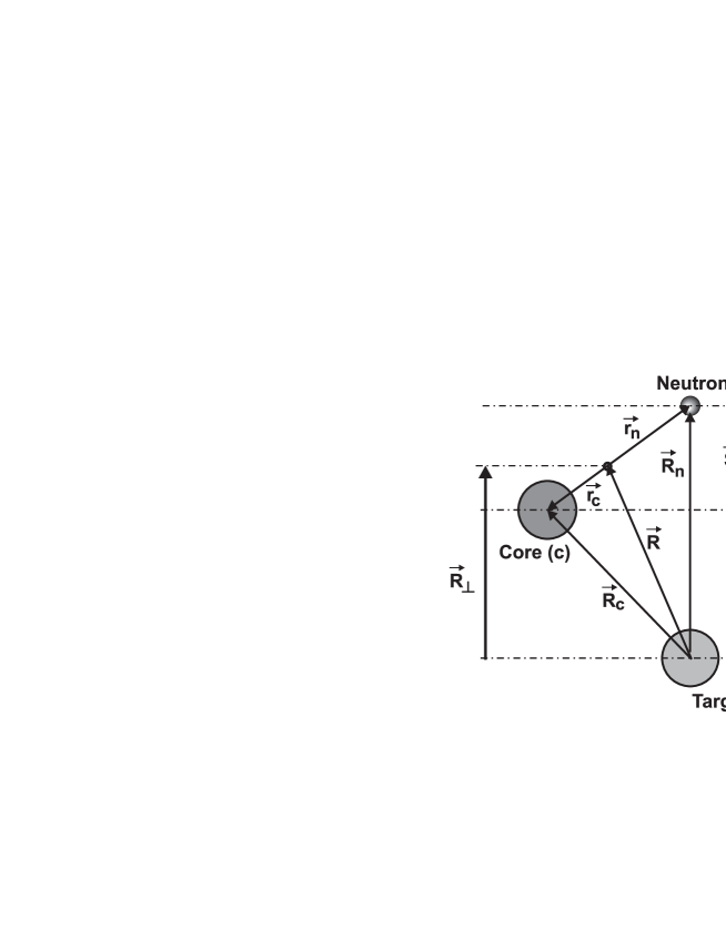
FIG. 6.: Coordinate system used in the Glauber model calculations.

FIG. 7.: $RMS$ matter radii extracted from Hartree-Fock + BCS calculations of single particle densities (black line), compared with experimental values from Liatard et al.[62] (filled circles), Ozawa et al.[66] (open circles) and Tanihata et al.[67] (open diamonds). The relativistic mean field calculations of Ren et al.[63, 64, 65] are indicated by the dashed lines.

FIG. 8.: S-matrix, absorption profiles and transmission coefficients for n–¹²C (left panels) and ¹⁴C–¹²C (right panels) interactions at 30 MeV/nucleon obtained from the JLM folding model calculations. Results using the lowest order of the eikonal approximation are shown as a dotted line, those using the first order corrections by the dot-dashed line, and those using second order corrections by the solid line. For ¹⁴C+¹²C the calculations converge with the use of first order corrections.

FIG. 9.: The effect of noneikonal corrections on the distortion kernels (see the text for definitions) as a function of impact parameter $s$, for neutron absorption and diffraction, core (¹⁴C) absorption and for absorption of both the core and neutron by ¹²C at 30 MeV/nucleon. Dotted lines: lowest order eikonal approximation. Dashed-dotted lines: first order noneikonal corrections included. Solid line: second order corrections included.

FIG. 10.: Elastic (dotted), reaction (dash-dotted) and total (solid line) neutron cross sections for reaction on four targets as a function of incident energy. The calculations were performed using JLM microscopic potentials in the eikonal approximation. Non eikonal corrections up to second order were included and the effects are shown by thin continuous lines (the convention is as per the previous two figures) for Be, C and Si targets. For the Ta target, the eikonal series does not converge in the range of energies shown. The experimental data for the total, elastic and reaction cross sections (open and closed circles and open squares) were taken from refs. [69, 70]

FIG. 11.: Selected examples (see text) of the core fragment longitudinal momentum distributions obtained using the Carbon target showing the contributions from the different reaction mechanisms. The calculated distributions (thick solid lines) include the absorption (thin solid lines), diffraction (dashed) and Coulomb (dash-dotted) components.

FIG. 12.: Calculated absorption (solid lines) and diffraction (dashed lines) cross sections versus binding energy for $s$ and $d$-wave states of an A=17 system at 50 MeV/nucleon on a Carbon target using the JLM interaction and various orders of eikonal theory.

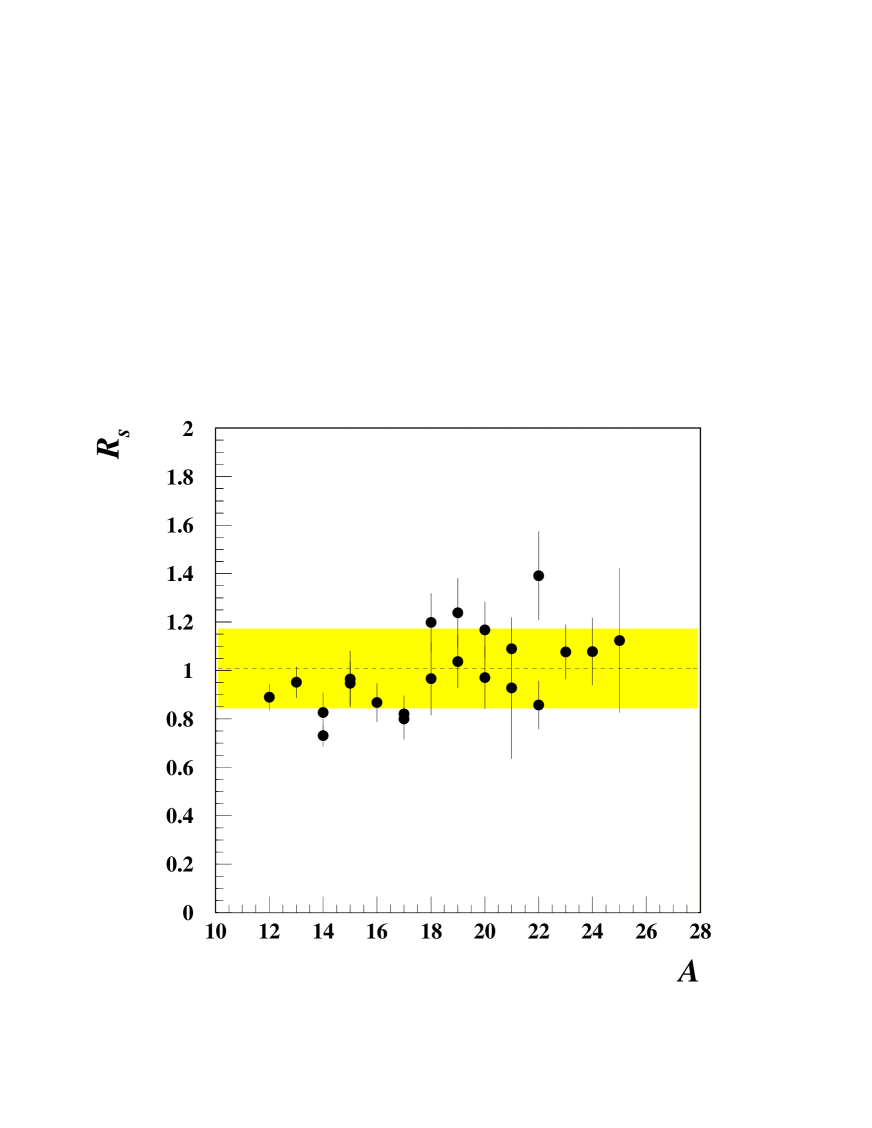
FIG. 13.: Ratio of experimental to theoretical cross sections ($R_{s}$) as a function of projectile mass number for the data obtained with the Carbon target. The dotted line indicates the mean value and the shadded band the 1$\sigma$ variance.

FIG. 14.: Test case calculations of the longitudinal ($k_{z}$) and transverse ($k_{x}$) core fragment momentum distributions for one-neutron removal by a Carbon target at 50 MeV/nucleon assuming an $s$, $p$ or $d$-wave state in an A=14 system with $S_{n}$= 1 MeV. The total (solid line), absorption (dashed), diffraction (dash-dotted) and Coulomb (dotted) components are indicated.

FIG. 15.: Correlations between the longitudinal and transverse ¹⁴C core fragment momenta for one-neutron removal from ¹⁵C by the Carbon target.

FIG. 16.: Core fragment transverse momentum distributions for one-neutron removal from ¹⁵C by the Tantalum target (filled circles). Dashed line: calculated transverse momentum distribution for Coulomb induced breakup. Solid line: same calculation after convolution with the orbital deflection in the Coulomb field of the target (see text for details).

FIG. 17.: Examples of the core fragment longitudinal momentum distributions for reactions on the Ta target. The filled circles represent the data. To aid in the comparison the calculated distributions for the total (solid lines), nuclear (dotted) and Coulomb dissociation (dashed line) are normalised to the data.

FIG. 18.: Comparison of the measured core fragment longitudinal momentum distributions (from reactions on the Carbon target) with those predicted for different projectile ground state spin-parity assignments. The favoured assignements are displayed as solid lines (see text).

FIG. 19.: Comparison of the measured ¹⁶C core fragment transverse momentum distribution for reactions of ¹⁷C on the Carbon target with the distributions calculated for the three possible ground state spin-parity assignments.

REFERENCES

- [1] D. K. Scott, Prog. in Part. Nucl. Phys. , 5 (1980) and references therein.
- [2] R. G. Stokstad, Comments Nucl. Part. Phys. , 231 (1984).
- [3] D. E. Greiner et al., Phys. Rev. Lett. , 152 (1975).
- [4] D. L. Olson et al., Phys. Rev. , 1602 (1983).
- [5] A. S. Goldhaber, Phys. Lett. , 306 (1974).
- [6] J. Hüfner and M. C. Nemes, Phys. Rev. , 2538 (1981).
- [7] W. A. Friedmann, Phys. Rev. , 569 (1983).
- [8] see, for example, N. A. Orr, Nucl. Phys. , 155 (1997) and references therein.
- [9] R. Serber, Phys. Rev. , 1008 (1947).
- [10] R. Anne et al., Phys. Lett. , 55 (1993).
- [11] R. Anne et al., Nucl. Phys. , 125 (1994).
- [12] N. A. Orr et al., Phys. Rev. Lett. , 2050 (1992).
- [13] N. A. Orr et al., Phys. Rev. , 3116 (1995).
- [14] J. H. Kelley et al., Phys. Rev. Lett. , 30 (1995).
- [15] H. Sagawa and K. Yazaki, Phys. Lett. , 149 (1990).
- [16] H. Sagawa and N. Takigawa, Phys. Rev. , 985 (1994).
- [17] P. G. Hansen, Phys. Rev. Lett , 1016 (1996).
- [18] H. Esbensen, Phys. Rev. , 2007 (1996); H. Esbensen, in Extremes of Nucl. Structure, Proc. Int. Workshop XXIV, Hirschegg on Extremes of Nuclear Structure, eds H. Feldmeyer, J. Knoll, W. Norenberg (GSI, Darmstadt, 1996) p321.
- [19] M. S. Hussein and K. W. McVoy, Nucl. Phys. , 123 (1985).
- [20] K. Hencken, G. Bertsch and H. Esbensen, Phys. Rev. , 3043 (1996).
- [21] Y. Ogawa and I. Tanihata, Nucl. Phys. , 239c (1997).
- [22] F. Negoita et al., Phys. Rev. , 2082 (1999).
- [23] J. A. Tostevin, J. Phys. G: Nucl. Part. Phys. , 735 (1999).
- [24] K. Yabana, Y. Ogawa and Y. Suzuki, Nucl. Phys. , 295 (1992).
- [25] Yu.L. Parfenova, M.V. Zhukov and J.S. Vaagen, Phys. Rev. , 044602-1 (2000).
- [26] A. Bonaccorso, D. M. Brink, Phys. Rev. , 1559 (1991).
- [27] P. G. Hansen and B. M. Sherrill, Nucl. Phys. , 133 (2001).
- [28] A. Navin et al., Phys. Rev. Lett. , 5089 (1998).
- [29] T. Aumann et al., Phys. Rev. Lett. , 35 (2000).
- [30] V. Guimarães et al., Phys. Rev. , 064609 (2000).
- [31] A. Navin et al., Phys. Rev. Lett. , 266 (2000).
- [32] V. Maddalena et al., Phys. Rev. C62, 024613 (2001).
- [33] D. Cortina-Gil et al., Phys. Lett. B529, 36 (2002).
- [34] J. Enders et al., Phys. Rev. C65, 034318 (2002).
- [35] P. G. Hansen and J. A. Tostevin, Ann. Rev. Nucl. Part. Sci. 53, in press.
- [36] J. Enders et al., Phys. Rev. C67, 064301 (2003).
- [37] J. A. Tostevin, in Proc. of the 2nd International Conference on Fission and Neutron Rich Nuclei, ed. W. Philips, (World Scientific) p. 735 (1999).
- [38] T. Baumann et al., Phys. Lett. , 256 (1998).
- [39] E. Sauvan et al., Phys. Lett. , 1 (2000).
- [40] R. Anne, Nucl. Inst. Meth. , 279 (1997).
- [41] L. Bianchi et al., Nucl. Inst. Meth. , 509 (1989).
- [42] K. Riisager, in Proc. of the 3rd Int. Conference on Radioactive Nuclear Beams, ed. D. J. Morrissey (Editions Frontières, Gif-sur-Yvette, 1993) p281.
- [43] K. Riisager, Habilitation Thesis, University of Aarhus (1994).
- [44] J. H. Kelley et al., Nucl. Inst. Meth. ,492 (1997).
- [45] E. Sauvan, Thèse, Université de Caen (2000), LPCC T00-01.
- [46] F. Carstoiu, E. Sauvan and N. A. Orr, to be published.
- [47] J. D. Silk et al., Phys. Rev. , 158 (1988).
- [48] D. Bazin et al., Phys. Rev. Lett. , 3569 (1995).
- [49] D. Bazin et al., Phys. Rev. , 2156 (1998).
- [50] T. Yamaguchi et al., Nucl. Phys. A724, 3 (2003).
- [51] R. Kanungo et al., Phys. Rev. Lett. , 142502 (2002).
- [52] D. Cortina-Gil et al., Eur. Phys. J. A10, 49 (2001).
- [53] D. Cortina-Gil, priv. comm.
- [54] G. Bertsch, H. Esbensen and A. Sustich, Phys. Rev. , 758 (1990).
- [55] A. Bonaccorso and G. F. Bertsch, Phys. Rev. , 044604 (2001).
- [56] C. A. Bertulani and G. Baur, Nucl. Phys. , 615 (1988).
- [57] A. Winther and K. Adler, Nucl. Phys. , 518 (1979).
- [58] A. Bonaccorso and F. Carstoiu, Phys. Rev. , 034605 (2000).
- [59] J. P. Jeukenne, A. Lejeune and C. Mahaux, Phys. Rev. , 80 (1977).
- [60] L. Trache et al., Phys. Rev. , 024612 (2000).
- [61] M. Beiner and R. J. Lombard, Ann. Phys. , 262 (1974).
- [62] E. Liatard et al., Europhys. Lett. , 401 (1990).
- [63] Zhongzhou Ren et al., Phys. Rev. , R20 (1995).
- [64] Zhongzhou Ren et al., Nucl. Phys. , 75 (1996).
- [65] Zhongzhou Ren et al., J. Phys. G: Nucl. Part. Phys. 22, L1 (1996).
- [66] A. Ozawa et al., Nucl. Phys. , 599 (2001).
- [67] I. Tanihata et al., Phys. Lett. , 592 (1988).
- [68] J. S. Wallace, Ann. Phys. (N.Y.) , 190 (1973).
- [69] http://www.nndc.bnl.gov
- [70] M. B. Chadwick, L. J. Cox, P. G. Young and A. S. Mengooni, Nucl. Sci. Eng. 123, 17 (1996).
- [71] B. A. Brown, A. Etchegoyen, W. D. M. Rae, Report MSUCL-524 (November 1988); http://www.nscl.msu.edu/ brown/
- [72] E. K. Warburton, B. A. Brown, Phys. Rev. , 923 (1992).
- [73] E. K. Warburton, B. A. Brown, D. J. Millener, Phys. Lett. , 7 (1992).
- [74] D. J. Millener and D. Kurath, Nucl. Phys. , 315 (1975).
- [75] F. Ajzenberg-Selove, Nucl. Phys. , 1 (1982).
- [76] F. Ajzenberg-Selove, Nucl. Phys. , 1 (1986).
- [77] F. Ajzenberg-Selove, Nucl. Phys. , 1 (1987).
- [78] P. M. Endt, Nucl. Phys. , 1 (1990).
- [79] V. Maddalena and R. Shyam, Phys. Rev. , 051601(R) (2001).
- [80] N. A. Orr et al., in Proc. of the 3rd Int. Conference on Radioactive Nuclear Beams, ed. D.J. Morrissey (Editions Frontières, Gif-sur-Yvette, 1993) p389.
- [81] W. N. Catford et al., Nucl. Phys. , 263 (1989).
- [82] N. A. Orr et al., Nucl. Phys. A491, 457 (1989).
- [83] D. R. Goosman Phys. Rev. C10, 756 (1974).
- [84] A. T. Reed et al., Phys. Rev. , 024311 (1999).
- [85] H. Ogawa et al., Eur. Phys. J. A13, 81 (2002).
- [86] J. Mougey et al., Phys. Lett. , 25 (1981).
- [87] J. Tostevin et al., Phys. Rev. , 024607 (2002).
- [88] A. Ozawa et al., Phys. Rev. Lett. , 5493 (2000).
- [89] B. A. Brown, P. G. Hansen, B. M. Sherrill and J. A. Tostevin Phys. Rev. C65, 061601(R) (2002).
- [90] V. R. Pandharipande, I. Sick and P. K. A. deWitt Huberts, Rev. Mod. Phys. , 981 (1997).
- [91] H. Esbensen and G. Bertsch, Phys. Rev. , 014608 (2001).
- [92] B. A. Brown et al., Phys. Rev. Lett. , 159201 (2003).
- [93] R. Kanungo et al., Phys. Rev. Lett. , 159202 (2003).
- [94] U. Datta Pramanik et al., Phys. Lett. B551, 63 (2003).
- [95] see, for example, G.R. Satchler, Direct Nuclear Reactions (Oxford University Press, Oxford, 1983).
- [96] G. J. Kramers, H. P. Blok and L. Lapikás, Nucl. Phys. , 267 (2001) and refs therein.
- [97] J. S. Winfield et al., Nucl. Phys. , 48 (2001).
A