Restoration of particle number as a good quantum number in BCS theory

Abstract

As shown in previous work, number projection can be carried out analytically for states defined in a quasi–particle scheme when the states are expressed in a coherent state representation. The wave functions of number–projected states are well–known in the theory of orthogonal polynomials as Schur functions. Moreover, the functions needed in pairing theory are a particularly simple class of Schur functions that are easily constructed by means of recursion relations. It is shown that complete sets of states can be projected from corresponding quasi–particle states and that such states retain many of the properties of the quasi–particle states from which they derive. It is also shown that number projection can be used to construct a complete set of orthogonal states classified by generalized seniority for any nucleus.

I Introduction

The loss of particle number as a good quantum number is a serious deficiency of the BCS and HFB (Hartree–Fock–Bogolyubov) approximations in their applications to finite nuclei. However, it can be restored with relative ease in a coherent-state representation [1, 2] in a manner that preserves much of the elegance and simplicity of the models.

Following early suggestions by Mottelson [3], number conserving extensions of BCS and HFB theory have been considered by many authors: cf., for example, the number-projected BCS approximation of Dietrich, Mang, and Pradal [4], the projected quasi-particle model of Lande, Ottaviani and Savoia [5], the antisymmetrized geminal power states of Coleman et al. [6], the broken pair model of Lorazo, Gambhir, and others [7, 8], Talmi’s generalized seniority scheme [9], and the coherent correlated pair method of Vary and Plastino [10]. A review of the subject has been given by Allaart et al. [11].

A common feature of these schemes is to approximate the ground state, for a system in which pair correlations dominate, by a state of the form

$$|{\cal N}\rangle=\Pi_{N}|x\rangle\,,$$ (1)

where $|x\rangle$ is a quasi-particle vacuum state and $\Pi_{N}$ is a projector onto the space of states of particle number $N$. We show herein that such a projection can be applied analytically, when the wave functions are expressed in a coherent-state representation. More importantly, projection from quasi-particle states gives a complete set of $N$-particle states which reflect many of the properties of the states from which they were projected. Thus, a potentially exact formalism emerges which is able to take advantage of the physical insights gained from the BCS and HFB approximations.

Analytic number projection when combined with analytic methods for projecting out states of good angular momentum from deformed intrinsic states [12] raises the possibility of developing good theories of nuclei which exhibit both rotational and superconducting properties. It also suggests a way of extending the physically significant definition of generalized seniority to the classification of complete sets of orthonormal states.

For simplicity, we restrict consideration in this paper to the BCS model. However, the methods extend to the general HB theory by the number projection methods given in ref. [1].

II Quasispin algebras and their coherent state representation

For each $j$-shell, there is an SU(2) quasispin algebra spanned by the operators

$$\hat{S}^{j}_{+}=\sum_{m=1/2}^{j}a^{\dagger}_{jm}a^{\dagger}_{j\bar{m}},\quad\hat{S}^{j}_{-}=\sum_{m=1/2}^{j}a^{j\bar{m}}a^{jm}\,,$$ (2)

$$\hat{S}^{j}_{0}=\displaystyle{1\over 4}\sum_{m=-j}^{j}(a^{\dagger}_{jm}a^{jm}-a^{jm}a^{\dagger}_{jm})\,,$$ (3)

where

$$a^{\dagger}_{j\bar{m}}=(-1)^{j-m}a^{\dagger}_{j,-m}\,,\quad a^{j\bar{m}}=(-1)^{j-m}a^{j,-m}=a_{jm}\,,$$ (4)

are creation and annihilation operators for a nucleon (e.g., neutron) which satisfy the fermion anticommutation relations

$$\{a^{jm},a^{\dagger}_{jn}\}=\delta_{mn}\,.$$ (5)

Note that we follow Einstein’s convention of using upper indices to label the components of a tensor contragredient to a tensor labeled by lower indices. With this convention, the annihilation operator $a^{jm}$ with superscripts is the Hermitian adjoint of the creation operator $a^{\dagger}_{jm}$ and the annihilation operator $a_{jm}$ with subscripts is the $m$ component of a spherical tensor. The contraction of a pair of upper and lower indices is then a scalar; e.g.,

$$\hat{n}_{j}=\sum_{m}a^{\dagger}_{jm}a^{jm}$$ (6)

is the number operator for the $j$-shell. The quasispin operators satisfy the usual SU(2) commutation relations

$$[\hat{S}^{j}_{+},\hat{S}^{j}_{-}]=2\hat{S}^{j}_{0}\,,\quad[\hat{S}^{j}_{0},\hat{S}^{j}_{\pm}]=\pm\hat{S}^{j}_{\pm}\,,$$ (7)

and the nucleon operators transform under SU(2) as components of quasispin–$1/2$ tensors:

$$\begin{array}[]{rcl}[\hat{S}^{j}_{-},a^{\dagger}_{jm}]=a_{jm},&&[\hat{S}^{j}_{+}\,,a_{jm}]=a^{\dagger}_{jm}\,,\cr[\hat{S}^{j}_{0},a^{\dagger}_{jm}]=\textstyle{1\over 2}a^{\dagger}_{jm}\,,&&[\hat{S}^{j}_{0},a_{jm}]=-\textstyle{1\over 2}a_{jm}\,.\cr\end{array}$$ (8)

Representations of a quasispin algebra are characterized by highest and lowest weights. For example, the zero-particle state $|0\rangle$ is a lowest weight state for all the quasispin algebras;

$$\hat{S}^{j}_{-}|0\rangle=0\,,\quad\hat{S}^{j}_{0}|0\rangle=-s_{j}|0\rangle\,,\quad\forall\,j\,,$$ (9)

where $s_{j}=(2j+1)/4$. Such a state is said to have multishell seniority $(0,0,\ldots)$. More generally, a state $|\nu JM\rangle$ of $\nu$ particles that satisfies the equations

$$\hat{S}^{j}_{-}|\nu JM\rangle=0\,,\quad\hat{S}^{j}_{0}|\nu JM\rangle=(-s_{j}+\nu_{j}/2)|\nu JM\rangle\,,\quad\forall\,j\,,$$ (10)

is said to have seniority $\nu$ and multishell seniority $(\nu_{j_{1}},\nu_{j_{2}},\ldots)$, where $\nu=\sum_{j}\nu_{j}$. The multishell seniority defines the values of the lowest weights and provides useful identifiers of the corresponding quasispin irreps.

A coherent state for the combined quasispin algebras is defined by

$$|x\nu\rho JM\rangle=e^{\hat{S}_{+}(x)}|\nu\rho JM\rangle\quad{\rm with}\quad\hat{S}_{+}(x)=\sum_{j}x_{j}\hat{S}^{j}_{+}\,,$$ (11)

where $|\nu\rho JM\rangle$ is a lowest weight state and $\rho$ provides whatever labels are needed, in addition to $\nu JM$, to characterize the state. A coherent state is a quasispin transform of a lowest weight state. The simplicity of the BCS and HFB theories stems from the fact that the quasi-particle operators of the Bogolyubov–Valatin transformation are also quasispin transforms of nucleon creation and annihilation operators. In particular, a coherent state of the seniority-zero irrep

$$|x\rangle=e^{\hat{S}_{+}(x)}|0\rangle$$ (12)

is the vacuum state of the quasi-particles defined, for real values of $\{x_{j}\}$, by the Bogolyubov–Valatin transformation

$$\begin{array}[]{c}\alpha^{\dagger}_{jm}=u_{j}a^{\dagger}_{jm}-v_{j}a_{jm}\,,\\ \alpha_{jm}=u_{j}a_{jm}+v_{j}a^{\dagger}_{jm}\,.\end{array}$$ (13)

with $u_{j}^{2}+v_{j}^{2}=1$ and $v_{j}=x_{j}u_{j}$. This well-known result follows from the observation that

$$\alpha_{jm}e^{\hat{S}_{+}(x)}=e^{\hat{S}_{+}(x)}(u_{j}a_{jm}+v_{j}a^{\dagger}_{jm}-x_{j}u_{j}a^{\dagger}_{jm})=u_{j}e^{\hat{S}_{+}(x)}a_{jm}\,.$$ (14)

Although the transformation $e^{\hat{S}_{+}(x)}$ is not unitary, it is simply related to the unitary transformation

$$g(x)=e^{\hat{S}_{+}(\beta)-\hat{S}_{-}(\beta)}\,,$$ (15)

for which

$$\cos\beta_{j}={1\over\sqrt{1+x_{j}^{2}}}=u_{j}\,,\quad\sin\beta_{j}={x_{j}\over\sqrt{1+x_{j}^{2}}}=v_{j}\,.$$ (16)

The relationship is given by the expansion

$$g(x)=e^{\hat{S}_{+}(x)}\prod_{j}(1+x_{j}^{2})^{\hat{S}^{j}_{0}}\,e^{-\hat{S}_{-}(x)}\,.$$ (17)

Thus, the transformation

$$|0\rangle\to|x\rangle=e^{\hat{S}_{+}(x)}|0\rangle=g(x)|0\rangle\,\prod_{j}(1+x_{j}^{2})^{s_{j}}$$ (18)

is unitary, to within a factor $\sqrt{\Phi^{s}(x^{2})}$, where

$$\Phi^{s}(x^{2})=\langle x|x\rangle=\prod_{j}(1+x_{j}^{2})^{2s_{j}}$$ (19)

and $x^{2}=(x_{j_{1}}^{2},x^{2}_{j_{2}},\ldots)$. Likewise, the BV transformation is seen as the unitary SU(2) transformation

$$a^{\dagger}_{jm}\to\alpha^{\dagger}_{jm}=g(x)a^{\dagger}_{jm}g^{\dagger}(x)\,,\quad a_{jm}\to\alpha_{jm}=g(x)a_{jm}g^{\dagger}(x)\,.$$ (20)

In a VCS (vector coherent state) representation [13, 14], a lowest weight state $|\nu\rho JM\rangle$ is regarded as an intrinsic state for an irrep of the combined quasi-spin algebras and represented by an intrinsic wave function $\xi_{\nu\rho JM}$. An arbitrary state $|\psi\rangle$ is then represented by a holomorphic wave function $\Psi$ defined over a set of complex coordinates $z=(z_{j_{1}},z_{j_{2}},\ldots)$ with values

$$\Psi(z)=\sum_{\nu\rho JM}\xi_{\nu\rho JM}\langle{\nu\rho JM}|e^{\hat{S}_{-}(z)}|\psi\rangle\,.$$ (21)

For example, if the zero-particle vacuum $|0\rangle$ has intrinsic wave function $\xi_{0}$, an arbitrary quasi-particle vacuum state $|x\rangle=e^{\hat{S}_{+}(x)}|0\rangle$ has wave function $\Psi_{x}$ with values

$$\Psi_{x}(z)=\xi_{0}\langle 0|e^{\hat{S}_{-}(z)}e^{\hat{S}_{+}(x)}|0\rangle=\xi_{0}\Phi^{s}(zx)\,,$$ (22)

where $\Phi^{s}(zx)$ is the overlap

$$\Phi^{s}(zx)=\langle z|x\rangle=\prod_{j}(1+z_{j}x_{j})^{2s_{j}}$$ (23)

with $zx=(z_{j_{1}}x_{j_{1}},z_{j_{2}}x_{j_{2}},\ldots)$. It follows that the norm of a quasi-particle vacuum state $|x\rangle$ is the value of the function $\Phi^{s}$ at $x^{2}$.

In the VCS representation, an element $\hat{X}$ of an SU(2) quasispin algebra is represented as a differential operator $\Gamma(\hat{X})$ defined by

$$[\Gamma(\hat{X})\Psi](z) = \sum_{\nu\rho JM}\xi_{\nu\rho JM}\langle{\nu\rho JM}|e^{\hat{S}_{-}(z)}\hat{X}|\psi\rangle$$ (24)

$$= \sum_{\nu\rho JM}\xi_{\nu\rho JM}\langle{\nu\rho JM}|\big{(}\hat{X}+[\hat{S}_{-}(z),X]$$ (26)

$$\quad+\textstyle{1\over 2}[\hat{S}_{-}(z),[\hat{S}_{-}(z),X]]\big{)}e^{\hat{S}_{-}(z)}|\psi\rangle\,.$$

Evaluation of the right hand side of this expression by means of the identities

$$\langle{\nu\rho JM}|\hat{S}_{+}^{j}e^{\hat{S}_{-}(z)}|\psi\rangle=0\,,\quad\langle{\nu\rho JM}|\hat{S}_{0}^{j}e^{\hat{S}_{-}(z)}|\psi\rangle=(-s_{j}+\nu_{j}/2)\Psi(z)\,,$$ (27)

$$\displaystyle\langle{\nu\rho JM}|\hat{S}_{-}^{j}e^{\hat{S}_{-}(z)}|\psi\rangle={\partial\over\partial z_{j}}\Psi(z)\,,$$ (28)

gives the representation

$$\Gamma(\hat{S}^{j}_{0})=-\hat{s}_{j}+z_{j}{\partial\over\partial z_{j}}\,,\quad\Gamma(\hat{S}^{j}_{-})={\partial\over\partial z_{j}}\,,\quad\Gamma(\hat{S}^{j}_{+})=z_{j}\Big{(}2\hat{s}_{j}-z_{j}{\partial\over\partial z_{j}}\Big{)}\,,$$ (29)

where $\hat{s}_{j}$ is a diagonal operator on intrinsic wave functions with eigenvalues

$$\hat{s}_{j}\xi_{\nu\rho JM}=(-s_{j}+\nu_{j}/2)\xi_{\nu\rho JM}\,.$$ (30)

The number operator $\hat{n}_{j}$ is represented

$$\Gamma(\hat{n}_{j})=\hat{\nu}_{j}+2z_{j}{\partial\over\partial z_{j}}\,.$$ (31)

III Number-projected states

Let $|n(x)\rangle$ denote the $n$-pair state

$$|n(x)\rangle=\big{[}S_{+}(x)\big{]}^{n}|0\rangle=n!\,\Pi_{2n}\,|x\rangle\,.$$ (32)

States of good nucleon number can also be projected from excited quasi-particle states. Consider first the one quasi-particle state $\alpha^{\dagger}_{jm}|x\rangle$. To within a factor $u_{j}=1/\sqrt{1+x_{j}^{2}}$, the $(2n+1)$-particle component of such a state is given by

$$u_{j}\Pi_{2n+1}\alpha^{\dagger}_{jm}|x\rangle=\Pi_{2n+1}e^{\hat{S}_{+}(x)}[u_{j}^{2}+x_{j}u_{j}v_{j}]a^{\dagger}_{jm}|0\rangle={1\over n!}\big{[}S_{+}(x)\big{]}^{n}|jm\rangle\,,$$ (33)

where $|jm\rangle=a^{\dagger}_{jm}|0\rangle$. This is a special case of a general result.

Claim 1: Let $Z_{\mu\beta JM}^{\dagger}(a^{\dagger})$ denote some combination of $\mu$ nucleon creation operators

$$Z_{\mu\beta JM}^{\dagger}(a^{\dagger})=\sum_{j}C^{j_{1},\ldots,j_{\mu}}_{\mu\beta JM}[a^{\dagger}_{j_{1}}\otimes a^{\dagger}_{j_{2}}\otimes\cdots\otimes a^{\dagger}_{j_{\mu}}]_{JM}$$ (34)

which creates a state

$$|\mu\beta JM\rangle=Z_{\mu\beta JM}^{\dagger}(a^{\dagger})|0\rangle$$ (35)

having the property that

$$\hat{S}_{-}(uv)|\mu\beta JM\rangle=0\,;$$ (36)

the subscript $\beta$ provides whatever labels are needed in addition to $\mu JM$ to specify the state. Let $Z_{\mu\beta JM}^{\dagger}(u\alpha^{\dagger})$ denote the corresponding quasi-particle operator in which each $a^{\dagger}_{jm}$ is replaced by $u_{j}\alpha^{\dagger}_{jm}$. Then

$$\Pi_{2n+\mu}Z_{\mu\beta JM}^{\dagger}(u\alpha^{\dagger})|x\rangle={1\over n!}\big{[}S_{+}(x)\big{]}^{n}|\mu\beta JM\rangle\,.$$ (37)

Proof: The claim follows from the identity

$$u_{j}\alpha^{\dagger}_{jm}e^{\hat{S}_{+}(x)}=e^{\hat{S}_{+}(x)}(a^{\dagger}_{jm}-u_{j}v_{j}a_{jm})=e^{\hat{S}_{+}(x)}e^{-\hat{S}_{-}(uv)}a^{\dagger}_{jm}e^{\hat{S}_{-}(uv)}$$ (38)

which implies that

$$Z_{\mu\beta JM}^{\dagger}(u\alpha^{\dagger})|x\rangle=e^{\hat{S}_{+}(x)}e^{-\hat{S}_{-}(uv)}Z_{\mu\beta JM}^{\dagger}(a^{\dagger})|0\rangle=e^{\hat{S}_{+}(x)}|{\mu\beta JM}\rangle\,.$$ (39)

Q.E.D.

It will be noted that to obtain complete sets of linearly independent states by number projection in this way, the states $\{|\mu\beta JM\rangle\}$ should include not only states that satisfy

$$\hat{S}^{j}_{-}|\mu\beta JM\rangle=0\quad\forall j\,,$$ (40)

but also states such as $\hat{S}_{+}(y)|\mu-2,\beta^{\prime}JM\rangle$ for $y\not=x$. Imposing the constraint

$$\hat{S}_{-}(uv)\hat{S}_{+}(y)|\mu-2,\beta^{\prime}JM\rangle=0$$ (41)

for all such states is one way, but not the only way, of ensuring that no linear combination of such states is of the form $\hat{S}_{+}(x)|\mu-2,\beta^{\prime}JM\rangle$. The latter states are not needed because the $(2n+\mu)$-particle states projected from $e^{\hat{S}_{+}(x)}\hat{S}_{+}(x)|\mu-2,\beta^{\prime}JM\rangle$ are proportional to those projected from $e^{\hat{S}_{+}(x)}|\mu-2,\beta^{\prime}JM\rangle$.

The above results lead to the following claim.

Claim 2: Let $\{Z^{\dagger}_{\mu\beta JM}(a^{\dagger})|0\rangle\}$ denote a complete set of orthonormal states, as defined in Claim 1, that satisfy the constraint $\hat{S}_{-}(uv)Z_{\mu\beta JM}^{\dagger}(a^{\dagger})|0\rangle=0$. Then the $N$-particle states number-projected from the corresponding quasi-particle states $\{Z^{\dagger}_{\mu\beta JM}(\alpha^{\dagger})|x\rangle\}$ form a (nonorthonormal) basis for the $N$-particle nucleus.

IV VCS wave functions of number-projected states

The number-projected state $|n(x)\rangle$ has VCS wave function

$$\Psi_{n(x)}(z)=\xi_{0}\langle 0|e^{\hat{S}_{-}(z)}|n(x)\rangle=\xi_{0}\Phi^{s}_{n}(zx)\,,$$ (42)

where $\Phi^{s}_{n}=n!P_{n}\Phi^{s}$ and $P_{n}\Phi^{s}$ is the component of $\Phi^{s}$ of degree $n$ in its argument. It turns out, as shown in refs. [1, 2] that the function $\Phi^{s}_{n}$ is well-known in the theory of symmetric polynomials [15] as a Schur function (or S-function); such functions are the characters of fully antisymmetric irreps of the unitary groups and easy to derive.

The definition

$$\Phi^{s}_{n}(zx)=\langle 0|e^{\hat{S}_{-}(z)}[\hat{S}_{+}(x)]^{n}|0\rangle$$ (43)

implies that

$$\Phi^{s}_{n}(zx)=[\Gamma(\hat{S}_{+}(x))\Phi^{s}_{n-1}](zx)\,.$$ (44)

where

$$\Gamma(\hat{S}_{+}(x))=\sum_{j}x_{j}\Gamma(\hat{S}^{j}_{+}))=\sum_{j}x_{j}z_{j}\Big{(}2s_{j}-z_{j}{\partial\over\partial z_{j}}\big{)}\,.$$ (45)

Thus, the needed Schur functions satisfy

$$\Phi^{s}_{n}(z)=\sum_{j}z_{j}\Big{(}2s_{j}-z_{j}{\partial\over\partial z_{j}}\Big{)}\Phi^{s}_{n-1}(z)\,.$$ (46)

Following the methods of ref. [1, 2], this recursion relation is solved by making a change of variables from $\{z_{j}\}$ to the symmetric power functions

$$\phi^{s}_{m}=\sum_{j}2s_{j}z_{j}^{m}\,.$$ (47)

The recursion relation then becomes

$$\Phi^{s}_{n}=\Big{[}\phi^{s}_{1}-\sum_{m}^{n-1}m\,\phi^{s}_{m+1}\nabla^{s}_{m}\Big{]}\Phi^{s}_{n-1}\,,$$ (48)

where

$$\nabla^{s}_{m}={\partial\over\partial\phi^{s}_{m}}\,,$$ (49)

and has solutions

$$\begin{array}[]{ccl}\Phi^{s}_{0}&=&1\\ \Phi^{s}_{1}&=&\phi^{s}_{1}\\ \Phi^{s}_{2}&=&(\phi^{s}_{1})^{2}-\phi^{s}_{2}\\ \Phi^{s}_{3}&=&(\phi^{s}_{1})^{3}-3\phi^{s}_{1}\phi^{s}_{2}+2\phi^{s}_{3}\,,\quad{\rm etc.}\\ \end{array}$$ (50)

The general expression is obtained by means of the identity

$$\nabla^{s}_{m}\Phi^{s}_{n}=(-1)^{m+1}{1\over m}{n!\over(n-m)!}\Phi^{s}_{n-m}\,,$$ (51)

derived in ref. [1]. With this identity, the recursion relation is given in the useful form

$$\Phi^{s}_{n}=\sum_{m=1}^{n}(-1)^{m+1}{(n-1)!\over(n-m)!}\phi^{s}_{m}\Phi^{s}_{n-m}$$ (52)

and has explicit solution given by

$$\Phi^{s}_{n}=\det\left|\matrix{\phi^{s}_{1}&1&0&0&\cdots&0\cr\phi^{s}_{2}&\phi^{s}_{1}&2&0&\cdots&0\cr\phi^{s}_{3}&\phi^{s}_{2}&\phi^{s}_{1}&3&\cdots&0\cr&&\cdots&&\cr\phi^{s}_{n}&\phi^{s}_{n-1}&\phi^{s}_{n-2}&\phi^{s}_{n-3}&\cdots&\phi^{s}_{1}\cr}\right|\,.$$ (53)

Some properties of these functions are discussed in refs. [1, 2, 15].

It follows from Claim 1 that the VCS wave function for a one quasi-particle state $u_{j}\alpha^{\dagger}_{jm}|x\rangle$ has values given by

$$\Psi_{x1jm}(z)=\xi_{jm}\langle 0|a^{jm}e^{\hat{S}_{-}(z)}e^{\hat{S}_{+}(x)}a^{\dagger}_{jm}|0\rangle\,.$$ (54)

From the observation that

$$\hat{S}_{-}^{k}a^{\dagger}_{jm}|0\rangle = 0\quad\forall k\,,$$ (55)

$$\hat{S}_{0}^{k}a^{\dagger}_{jm}|0\rangle = (-s_{k}+\textstyle{1\over 2}\delta_{kj})a^{\dagger}_{jm}|0\rangle$$ (56)

it follows that

$$\Psi_{x1jm}(z)=\xi_{jm}\Phi^{j}(zx)\,,$$ (57)

where

$$\Phi^{j}(z)=(1+z_{j})^{2s_{j}-1}\prod_{k\not=j}(1+z_{k})^{2s_{k}}\,.$$ (58)

This function has values

$$\Phi^{j}(z)={1\over 1+z_{j}}\Phi^{s}(z)=\Phi^{s^{\prime}}(z)\,,$$ (59)

where $s^{\prime}$ is the set of quasi-spins with

$$s^{\prime}_{k}=s_{k}-\textstyle{1\over 2}\delta_{kj}\,.$$ (60)

Thus, by considering $\Phi^{s}$ to be one of a set of functions parameterized by values $\{s_{j}=(2j+1)/4\}$ of the quasispins, $\Phi^{j}$ is seen to be the member of the set with $s_{j}$ replaced by $s_{j}-1/2$. This substitution will be denoted by an operator $\Delta^{j}$, i.e.,

$$\Delta^{j}:s_{j}\to s_{j}-\textstyle{1\over 2}\,,$$ (61)

so that

$$\Phi^{j}=\Delta^{j}\Phi^{s}\,.$$ (62)

The adjustment of the coherent state wave function $\Phi^{s}\to\Phi^{j}$ by the replacement $s_{j}\to s_{j}-1/2$ to take account of the occupation of one state of a single-particle level is an expression of the well-known blocking effect.

The number-projected one quasi-particle state

$$|n(x)1jm\rangle=n!u_{j}\Pi_{2n+1}\alpha^{\dagger}_{jm}|x\rangle=[\hat{S}_{+}(x)]^{n}a^{\dagger}_{jm}|0\rangle$$ (63)

is now seen to have VCS wave function with

$$\Psi_{n(x)1jm}(z)=n!\xi_{jm}P_{n}\Phi^{j}(zx)=\xi_{jm}\Phi^{j}_{n}(zx)\,,$$ (64)

where $\Phi^{j}_{n}$ is the Schur function

$$\Phi^{j}_{n}=\Delta^{j}\Phi^{s}_{n}\,.$$ (65)

Similarly, VCS wave functions are derived for all other number-projected quasi-particle states. For example, the seniority two states projected from a two quasi-particle state $n!u_{j_{1}}u_{j_{2}}[\alpha^{\dagger}_{j_{1}}\otimes\alpha^{\dagger}_{j_{2}}]_{JM}|x\rangle$ with $J\not=0$ have wave functions

$$\Psi_{n(x)(j_{1}j_{2})JM}(z)=[\xi_{j_{1}}\otimes\xi_{j_{2}}]_{JM}\Phi^{j_{1}j_{2}}_{n}(zx)\,,$$ (66)

where

$$\Phi^{j_{1}j_{2}}_{n}=\Delta^{j_{1}}\Delta^{j_{2}}\Phi^{s}_{n}=\Phi^{s^{\prime\prime}}_{n}$$ (67)

is the Schur function for the quasi-spin set $s^{\prime\prime}$ with components

$$s^{\prime\prime}_{k}=s_{k}-\textstyle{1\over 2}(\delta_{kj_{1}}+\delta_{kj_{2}})\,.$$ (68)

The seniority-zero state $\hat{S}_{+}(y)|n(x)\rangle$ has VCS wave function given by

$$\xi_{0}\sum_{j}y_{j}z_{j}\Big{(}2s_{j}-z_{j}{\partial\over\partial z_{j}}\big{)}\Phi^{s}_{n}(zx)=\xi_{0}\big{[}\phi^{s}_{1}(\tilde{y})-\sum_{m}m\phi_{1}(\tilde{y}\tilde{x}^{m})\nabla_{m}]\Phi^{s}_{n}(\tilde{x})\,,$$ (69)

where $\tilde{x}=xz$ and $\tilde{y}=yz$. Thus, with the identity (51), the VCS wave function for the state $\hat{S}_{+}(y)|n(x)\rangle$ is given by

$$\xi_{0}\langle 0|e^{\hat{S}_{-}(z)}\hat{S}_{+}(y)|n(x)\rangle=\xi_{0}\sum_{m=0}^{n}(-1)^{m}{n!\over(n-m)!}\phi_{1}(\tilde{y}\tilde{x}^{m})\Phi_{n-m}(\tilde{x})\,.$$ (70)

As expected, this wave function becomes identical to $\xi_{0}\Phi^{s}_{n+1}$ when $y=x$.

V Evaluation of energies and matrix elements

To illustrate the techniques, we consider the simple BCS Hamiltonian

$$H=\sum_{j}\varepsilon_{j}\hat{n}_{j}-G\hat{S}_{+}\hat{S}_{-}\,,$$ (71)

with

$$\hat{n}_{j}=\sum_{m}a^{\dagger}_{jm}a^{jm}\,,\quad\hat{S}_{\pm}=\sum_{j}\hat{S}^{j}_{\pm}\,.$$ (72)

For given real values of $x=(x_{j_{1}},x_{j_{2}},\ldots)$, the quasi-particle operators are defined by

$$\begin{array}[]{c}\alpha^{\dagger}_{jm}=u_{j}a^{\dagger}_{jm}-v_{j}a_{jm}\,,\\ \alpha_{jm}=u_{j}a_{jm}+v_{j}a^{\dagger}_{jm}\,,\\ \end{array}$$ (73)

such that $u_{j}^{2}+v_{j}^{2}=1$ and $v_{j}=x_{j}u_{j}$ so that

$$u_{j}^{2}={1\over 1+x^{2}_{j}}\,,\quad u_{j}v_{j}={x_{j}\over 1+x_{j}^{2}}\,,\quad v_{j}^{2}={x_{j}^{2}\over 1+x_{j}^{2}}\,.$$ (74)

A The number-projected vacuum energy

From standard BCS theory, the expectation of $H$ for a quasi-particle vacuum state is given by

$$\langle x|H|x\rangle=\Big{[}\sum_{j}2s_{j}(2\varepsilon_{j}-Gv_{j}^{2})v_{j}^{2}-G\Big{(}\sum_{j}2s_{j}u_{j}v_{j}\Big{)}^{2}\,\Big{]}\Phi^{s}(x^{2})\,.$$ (75)

With the above expressions for $u_{j}$ and $v_{j}$, this expression becomes

$$\langle x|H|x\rangle = \Big{[}\sum_{j}2\varepsilon_{j}{2s_{j}x^{2}_{j}\over 1+x^{2}_{j}}-G\sum_{j}{2s_{j}x_{j}^{4}\over(1+x^{2}_{j})^{2}}-G\Big{(}\sum_{j}{2s_{j}x_{j}\over 1+x^{2}_{j}}\Big{)}^{2}\,\Big{]}\Phi^{s}(x^{2})$$ (76)

$$= \sum_{j}4s_{j}\varepsilon_{j}x^{2}_{j}\Phi^{j}(x^{2})-G\sum_{j}2s_{j}x_{j}^{4}\Phi^{jj}(x^{2})$$ (78)

$$-G\sum_{ij}4s_{i}s_{j}x_{i}x_{j}\Phi^{ij}(x^{2})\,.$$

The energy of the $n$-pair state $|n(x)\rangle$,

$$E_{0}^{n}(x)={\langle x|H|n(x)\rangle\over\langle x|n(x)\rangle}\,,$$ (79)

is now obtained by picking out the components of $\langle x|H|x\rangle$ and $\langle x|x\rangle$ of degree $n$ in $x^{2}$. Recalling that $P_{2n}\Phi^{s}=\Phi^{s}_{n}/n!$, we immediately obtain

$$E_{0}^{n}(x) = {n\over\Phi^{s}_{n}(x^{2})}\sum_{j}\Big{[}4s_{j}\varepsilon_{j}x^{2}_{j}\Phi^{j}_{n-1}(x^{2})-G(n-1)2s_{j}x_{j}^{4}\Phi^{jj}_{n-2}(x^{2})$$ (81)

$$\qquad-G\sum_{i}4s_{i}s_{j}x_{i}x_{j}\Phi^{ij}_{n-1}(x^{2})\Big{]}\,.)$$

Thus, the values of the $x$ coefficients can be fixed such that the energy $E_{0}^{n}=E_{0}^{n}(x)$ is minimized and the variational equation

$${\partial\over\partial z_{j}}\,\langle z|(H-E_{0}^{n})|n(x)\rangle\Big{|}_{z=x}=0\,,\quad\forall\,j\,,$$ (82)

is satisfied.

B Number-projected one quasi-particle energies

As observed above, the $(2n+1)$-particle component of the one quasi-particle state $n!u_{j}\alpha^{\dagger}_{jm}|x\rangle$ is the state $|n(x)1jm\rangle=a^{\dagger}_{jm}|n(x)\rangle$. Thus, we consider the energies of number-projected one quasi-particle states defined by

$$E_{j}^{n}\,\langle n(x)1jm|n(x)1jm\rangle=\langle n(x)1jm|(H-E_{0}^{n})|n(x)1jm\rangle$$ (83)

or equivalently by

$$E_{j}^{n}\,\Phi^{j}_{n}(x^{2})=\langle x|a^{jm}(H-E_{0}^{n})a^{\dagger}_{jm}|n(x)\rangle\,.$$ (84)

Now the coherent state representation of the number operator $\hat{n}_{j}=\sum_{m}a^{\dagger}_{jm}a^{jm}$, when acting on a seniority zero state, is given by

$$\Gamma(\hat{n}_{j})\to 2z_{j}{\partial\over\partial z_{j}}\,.$$ (85)

Therefore

$$\langle x|a^{jm}a^{\dagger}_{jm}(H-E_{0}^{n})|n(x)\rangle = \Big{(}1-{z_{j}\over 2s_{j}}{\partial\over\partial z_{j}}\Big{)}\langle z|(H-E_{0}^{n})|n(x)\rangle\Big{|}_{z=x}$$ (86)

$$= 0$$ (87)

when $x$ is assigned the value for which eqn. (82) is satisfied. It follows that

$$E^{j}_{n}\,\Phi^{j}_{n}(x^{2})=\langle x|a^{jm}[H,a^{\dagger}_{jm}]|n(x)\rangle\,.$$ (88)

If we now (temporarily) regard $x$ as a variable parameter, we obtain from Claim 1 the identity

$$\langle x|a^{jm}[H,a^{\dagger}_{jm}]|n(x)\rangle = u_{j}\langle x|\alpha^{jm}[H,a^{\dagger}_{jm}]|n(x)\rangle$$ (89)

$$= n!P_{n}u_{j}\langle x|\alpha^{jm}[H,a^{\dagger}_{jm}]|x\rangle\,,$$ (90)

where $P_{n}$ picks out the component of degree $n$ in $x^{2}$ in what follows it. Note that for a particular value of $x$, the matrix element $\langle x|\alpha^{jm}[H,\alpha^{\dagger}_{jm}]|x\rangle$ is a number. However, by regarding $x$ first as a variable and evaluating the matrix element as a function of $x$, it is meaningful to extract the component of this function of degree $n$; the rhs of eqn. (90) is then the value of this component at the assigned value of $x$.

The quasi-particle vacuum properties of the state $|x\rangle$, which hold for arbitrary $x$, can now be used to put the matrix element on the right into the standard equations-of-motion form [16]

$$\langle x|\alpha^{jm}[H,a^{\dagger}_{jm}]|x\rangle=\langle x|\{\alpha^{jm},[H,a^{\dagger}_{jm}]\}|x\rangle\,.$$ (91)

This matrix element is then evaluated by BCS methods to give

$$u_{j}\langle x|\{\alpha^{jm},[H,a^{\dagger}_{jm}]\}|x\rangle=\big{[}\varepsilon_{j}u_{j}^{2}-Gu_{j}^{2}v_{j}^{2}+Gu_{j}v_{j}\sum_{i}2s_{i}u_{i}v_{i}\big{]}\Phi^{s}(x^{2})\,.$$ (92)

The final step of number projection is now easy and gives the expression for the number-projected one quasi-particle energies

$$E_{j}^{n}\Phi^{j}_{n}(x^{2})=\varepsilon_{j}\Phi^{j}_{n}(x^{2})-nGx^{2}_{j}\Phi^{jj}_{n-1}(x^{2})+nG\sum_{i}2s_{i}x_{i}x_{j}\Phi^{ij}_{n-1}(x^{2})\,.$$ (93)

This is an explicit and simple expression for $E_{j}^{n}$ which involves only the values of known (Schur) functions at the specific $x$ for which $E_{0}^{n}(x)$ is a minimum.

C Matrix elements between seniority-two states

Let $\{A^{\dagger}_{klJM}(a^{\dagger})|0\rangle\}$ be an orthonormal set of two-particle seniority-two states. The matrix elements between the corresponding number-projected quasi-particles states are given by

$$\langle x|A^{ijJM}HA^{\dagger}_{klJM}|n(x)\rangle=n!P_{n}\langle x|A^{ijJM}(u\alpha)HA^{\dagger}_{klJM}(u\alpha^{\dagger})|x\rangle\phantom{xxxxxxx}$$ (94)

$$=n!P_{n}\Big{(}\delta_{ij,kl}u_{k}^{2}u_{l}^{2}\langle x|H|x\rangle+\langle x|[A^{ijJM}(u\alpha),[H,A^{\dagger}_{klJM}(u\alpha^{\dagger})]]|x\rangle\Big{)}\,.$$ (95)

Thus, the matrix elements for seniority-two states are given by number projection of corresponding quasi-particle Tamm–Dancoff expressions, as defined in the equations-of-motion formalism [16]. Moreover, the projections are accomplished by expanding the unprojected expressions in terms of Schur functions.

D Matrix elements between seniority-zero states

After evaluating the overlaps $\langle x|\hat{S}_{-}(x)\hat{S}_{+}(y)|n(x)\rangle$ and $\langle x|\hat{S}_{-}(y)\hat{S}_{+}(y^{\prime})|n(x)\rangle$, one can construct an orthonormal set of seniority-zero states for a $2n$-particle nucleus. However, so that use can be made of Claim 1, it is convenient to start with operators $\{\hat{S}_{+}(y)\}$ that satisfy the condition

$$\hat{S}_{-}(uv)\hat{S}_{+}(y)|0\rangle=0\,.$$ (96)

The overlap $\langle x|\hat{S}_{-}(x)\hat{S}_{+}(y)|n(x)\rangle=(n+1)\langle x|\hat{S}_{+}(y)|n(x)\rangle$ is obtained from the value $\xi_{0}\langle x|\hat{S}_{+}(y)|n(x)\rangle$ at $z=x$ of the coherent state wave function for the state $S_{+}(y)|n(x)\rangle$; an expression for this wave function is given by eqn. (70). The second overlap is given by

$$\langle x|\hat{S}_{-}(y)\hat{S}_{+}(y^{\prime})|n(x)\rangle = \sum_{j,m>0}\sum_{j^{\prime},m^{\prime}>0}y_{j}y^{\prime}_{j^{\prime}}\langle x|a^{j\bar{m}}a^{jm}a^{\dagger}_{j^{\prime}m^{\prime}}a^{\dagger}_{j^{\prime}\bar{m}^{\prime}}|n(x)\rangle$$ (97)

$$= \sum_{j}2s_{j}y_{j}y^{\prime}_{j}\Phi^{jj}_{n}(x^{2})\,.$$ (98)

The matrix element $\langle x|\hat{S}_{-}(x)H\hat{S}_{+}(y)|n(x)\rangle=(n+1)\langle x|H\hat{S}_{+}(y)|n(x)\rangle$ is evaluated starting from the observation that

$$\langle x|(H-E_{0}^{n})\hat{S}_{+}(y)|n(x)\rangle = \langle n(x)|(H-E^{0}_{n})\hat{S}_{+}(y)|x\rangle$$ (99)

$$= \langle x|\hat{S}_{-}(y)(H-E^{0}_{n})|n(x)\rangle^{*}$$ (100)

and that

$$\langle z|\hat{S}_{-}(y)(H-E^{n}_{0})|n(x)\rangle=\sum_{j}y_{j}z_{j}\Big{(}2s_{j}-z_{j}{\partial\over\partial z_{j}}\Big{)}\langle z|(H-E^{n}_{0})|n(x)\rangle$$ (101)

vanishes when $z=x$ because of eqn. (82). It follows that

$$\langle x|\hat{S}_{-}(x)H\hat{S}_{+}(y)|n(x)\rangle=(n+1)E_{0}^{n}\langle x|\hat{S}_{+}(y)|n(x)\rangle\,.$$ (102)

Writing

$$\langle x|\hat{S}_{-}(y)H\hat{S}_{+}(y^{\prime})|n(x)\rangle=n!P_{n}\langle x|\hat{S}_{-}(y)H\hat{S}_{+}(y^{\prime})|x\rangle\,,$$ (103)

and defining

$$\tilde{S}_{-}(u^{2}y)=\sum_{j,m>0}u^{2}_{j}y_{j}a^{j\bar{m}}a^{jm}\,,\quad\tilde{S}_{+}(u^{2}y^{\prime})=\sum_{j,m>0}u^{2}_{j}y^{\prime}_{j}a^{\dagger}_{jm}a^{\dagger}_{j\bar{m}}\,,$$ (104)

we can use Claim 1 to obtain

$$\langle x|\hat{S}_{-}(y)H\hat{S}_{+}(y^{\prime})|n(x)\rangle=n!P_{n}\langle x|\tilde{S}_{-}(u^{2}y)H\hat{S}_{+}(u^{2}y^{\prime})|x\rangle\,.$$ (105)

Then, with the identity

$$\langle x|\tilde{S}_{-}(u^{2}y)\hat{S}_{+}(u^{2}y^{\prime})H|x\rangle=\sum_{j}2s_{j}u^{4}_{j}y_{j}y^{\prime}_{j}\langle x|H|x\rangle\,,$$ (106)

we obtain

$$\langle x|\hat{S}_{-}(y)H\hat{S}_{+}(y^{\prime})|n(x)\rangle = n!P_{n}\Big{[}\sum_{j}2s_{j}u^{4}_{j}y_{j}y^{\prime}_{j}\langle x|H|x\rangle$$ (108)

$$\quad+\langle x|[\tilde{S}_{-}(u^{2}y),[H\hat{S}_{+}(u^{2}y^{\prime})]]|x\rangle\Big{]}\,.$$

VI Generalized seniority

Talmi [9] has defined the sequence of $J=0$ states proportional to $\{[\hat{S}_{+}(x)]^{n}|0\rangle;$ $n=1,2,\ldots\}$ as states of generalized seniority zero. Likewise, the sequences of $J\not=0$ states $\{[\hat{S}_{+}(x)]^{n}|2JM\rangle;n=1,2,\ldots\}$, where $|2JM\rangle$ is a two-particle state that is annihilated by all the quasispin lowering operators (i.e., $\hat{S}^{j}_{-}|2JM\rangle$ $=0,\;\forall j$), are defined to be states of generalized seniority two. States of higher generalized seniority are similarly defined. Thus, the concept of generalized seniority identifies subsets of states of the corresponding seniority (more precisely summed multishell seniority $\nu=\sum_{j}\nu_{j}$). The generalized seniority zero states, for example, exclude states that are generated by combinations of the $\{\hat{S}^{j}_{+}\}$ operators that are not simply multiples of $\hat{S}_{+}(x)$. Such states, sometimes described as broken $\hat{S}_{+}(x)$ pair states [7], are also described as generalized seniority-two or higher states, depending on how many $\hat{S}_{+}(x)$ pairs are broken. The problem is that, while one can define two-particle $J=0$ parent states $\{|N=2,J=0\rangle\}$ as states that are annihilated by the $\hat{S}_{-}(x)$ lowering operators, in parallel with lowest-weight quasispin states, the sequences of states $\{[\hat{S}_{+}(x)]^{n}|2,J=0\rangle;n=1,2,\ldots\}$ are not orthogonal to the generalized seniority-zero states. Consequently, as Talmi has emphasized, generalized seniority does not define a complete orthogonal scheme.

Nevertheless, generalized seniority can be given a definition that does characterize a complete set of orthogonal states for each nucleus separately. For example, one can define a generalized seniority-two creation operator $\hat{S}_{+}(y)$ for the $2n$-particle nucleus such that

$$\langle x|\hat{S}_{+}(y)|n(x)\rangle=0\,.$$ (109)

With the identity

$$\langle z|\hat{S}_{+}(p)[\hat{S}_{+}(x)]^{n}|0\rangle=n!P_{n}\langle z|\hat{S}_{+}(yp)|x\rangle=n!P_{n}\sum_{j}y_{j}{\partial\over\partial x_{j}}\Phi^{s}(zx)\,,$$ (110)

this equation reduces to the easy to solve equation for the $y_{j}$ coefficients

$$\sum_{j}2s_{j}y_{j}x_{j}\Phi^{j}_{n}(x^{2})=0\,.$$ (111)

States of higher generalized seniority may be defined similarly.

Such a definition, has not been used to our knowledge probably because it would appear to destroy the simplicity and elegance of the concept. However, the facility to carry out number-projection analytically suggests that this may no longer be a significant concern.

VII Application to a two-level model

To check the above methods, they have been applied to a simple two-level model having Hamiltonian $H=\sum_{j}\varepsilon_{j}\hat{n}_{j}-G\hat{S}_{+}\hat{S}_{-}$ with $\varepsilon_{1}=0$ and $\varepsilon_{2}=1$; the excitation energy $\varepsilon_{2}-\varepsilon_{1}=1$ then sets the unit of the energy scale. For simplicity, we also set $s_{1}=s_{2}=s$ and considered a model nucleus with $n=2s$ nucleons; this corresponds to a situation in which, in the $G=0$ limit, the lower level is fully occupied and the upper level empty.

For such a two-level model, we can set

$$x_{1}=1\,,\quad x_{2}=x\,,$$ (112)

because replacing these parameters values by the substitution $x_{1}\to k$, $x_{2}\to kx$ would only change the overall norm of the state

$$|n(x)\rangle=[\hat{S}^{1}_{+}+x\hat{S}^{2}_{+}]^{n}|0\rangle\to k^{n}[\hat{S}^{1}_{+}+x\hat{S}^{2}_{+}]^{n}|0\rangle\,.$$ (113)

The energy $E^{n}_{0}(x)$ of the state, with $n=2s$, is then evaluated directly from eqn. (81) and the value of $x$, for which it is a minimum, determined.

The structure of the state $|n(x)\rangle$ is revealed by expanding it on a basis of states labeled by the two-level quasispin quantum numbers

$$\{|m\rangle=|s,s-m;s,m-s\rangle\,,\quad m=-s,\ldots,+s\}\,.$$ (114)

The state $|m\rangle$ is the state with m nucleon pairs in the upper level and $s-m$ pairs (or $m$ hole pairs) in the lower level. The expansion

$$|n(x)\rangle=\sum_{m=-s}^{s}C_{m}|m\rangle$$ (115)

in this basis is easily inferred from the identity

$$\Phi^{s}_{2s}(x^{2})=\langle x|n(x)\rangle\,,$$ (116)

which implies that the squares of the $C_{m}$ coefficients are given by the corresponding expansion of $\Phi^{s}_{2s}(x^{2})$ as a polynomial in $x^{2m}$;

$$\Phi^{s}_{2s}(x^{2})={1\over n!}\sum_{m}|C_{m}|^{2}x^{2m}\,.$$ (117)

The $C_{m}$ coefficients are shown, for $s=7/2$ and three values of $G$, in comparison with exactly computed wave functions for the model in fig. 1.

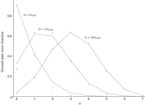
FIG. 1.: Ground state wave functions for $n=2s=14$ particles in a two–level pairing model for three values of the pairing interaction. The expansion coefficients, as defined in the text, for normalized number–projected states are shown as small circles. The corresponding coefficients for exactly computed ground states are connected by continuous lines.

For $s=7/2$, the model corresponds to 14 nucleons in two $j=13/2$ levels. Results computed for other values of $n=2s$ show that the number-projected wave functions rapidly become exact as $s\to\infty$.

As an indication of the improvement given by number projection over unprojected BCS results is given by comparing the ratio of the number of nucleons occupying the upper level to the number in the lower level. The mean number in the upper level is given for the above wave functions by

$$\langle n_{2}\rangle=\sum_{m}2m|C_{m}|^{2}x^{2m}\over\sum_{m}|C_{m}|^{2}x^{2m}$$ (118)

and the mean number for the lower level is

$$\langle n_{1}\rangle=2s-\langle n_{2}\rangle\,.$$ (119)

Fig. LABEL:fig:ratios shows the ratio $\langle n_{2}\rangle/\langle n_{1}\rangle$ for several values of the pairing interaction in comparison to the exact ratios and those of the BCS approximation.

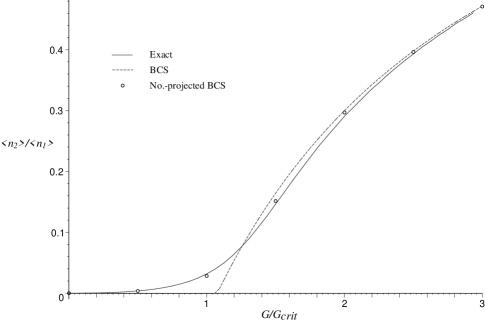
FIG. 2.: The ratio of the mean number of particles in the upper level to the mean number in the lower level for the $n=2s=14$ two–level pairing model defined in the text. The ratios for number–projected states are compared with exactly computed results and with those of the BCS approximation.

As $n=2s\to\infty$, the occupancies given by the BCS approximation are found to approach those of an exact calculation. However, for a finite number of particles, a considerable improvement is gained by number projection (as expected from previous results).

VIII Concluding remarks

The calculations that have been done, cf. for example refs. [2, 11], show clearly that number projection effects very substantial improvement to the accuracy of the BCS approximation in applications to finite nuclei. Moreover, the coherent state techniques introduced in refs. [1] and [2] were found to facilitate the practical steps of carrying out the number projection considerably. These techniques have been developed in this paper in the hope that they will be taken up by others in calculations of the low-energy spectra of nuclei in which pair-correlations are dominant. Of particular interest are the low-energy spectra of single-shell nuclei with both pairing and quadrupole interactions where the objective will be explore the emergence of deformed rotational states.

Other recent developments that may be usefully deployed in concert with number projection are: the identification of a range of seniority-conserving interactions [17], and analytic techniques to carry out angular momentum projection from a class of deformed intrinsic states [12].

REFERENCES

• [1] D.J. Rowe, T. Song, and H. Chen, Phys. Rev. C 44 (1991) R598.
• [2] H. Chen, T. Song, and D.J. Rowe, Nucl. Phys. A 582 (1995) 181.
• [3] B.R. Mottelson, in The many–body problem, (Dunod, Les Houches, 1958).
• [4] K. Dietrich, H.J. Mang, and J.H. Pradal, Phys. Rev. 135 (1964) B22.
• [5] A. Lande, Ann. Phys. 31 (1965) 525; P.L. Ottaviani and M. Savoia, Phys. Rev. 187 (1969) 1306; Nuovo Cim. 67A (1970) 630.
• [6] A.J. Coleman, J. Math. Phys. 6 (1965) 1425; J.V. Ortiz, B. Weaver, and Y.Öhrn, Int. J. Quantum Chem. Symp. 15 (1981) 113.
• [7] B. Lorazo, Phys. Lett. B 29 (1969) 150; Nucl. Phys. A 153 (1970) 255.
• [8] Y.K. Gambhir, A. Rimini, and T. Weber, Phys. Rev. 188 (1969) 1573; Phys. Rev. C 7 (1973) 1454.
• [9] I. Talmi, Nucl. Phys. A 172 (1971) 1; Phys. Lett. 55B (1975) 255.
• [10] J.P. Vary and A. Plastino, Phys. Rev. C 28 (1983) 2494.
• [11] K. Allaart, E. Boeker, G. Bonsignori, M. Savoia, and Y.K. Gambhir, Phys. Reports 169 (1988) 209.
• [12] D.J. Rowe, S.T. Bartlett, and C. Bahri, Phys. Lett. B 472, 227-231 (2000); R.M. Asherova. Yu.F. Smirnov, V.N. Tolstoy, and A.P. Shustov, Nucl. Phys. A355, 25 (1981).
• [13] D.J. Rowe, J. Math.  Phys. 25, 2662 (1984); D.J. Rowe, G. Rosensteel and R. Carr, J. Phys. A: Math. Gen. 17, L399 (1984); D.J. Rowe, G. Rosensteel and R. Gilmore, J. Math. Phys. 26, 2787 (1985).
• [14] D.J. Rowe and J. Repka, J. Math. Phys. 32, 2614 (1991).
• [15] I.G. Macdonald, Symmetric functions and Hall polynomials (Oxford, 1979).
• [16] D.J. Rowe, Rev. Mod. Phys.  40 (1968) 153; D.J. Rowe, “Nuclear Collective Motion; Models and Theory” (Methuen, London, 1970).
• [17] D.J. Rowe, “Partially solvable pair–coupling models and some challenges” (University of Toronto preprint).