Quasiclassical Born-Oppenheimer approximations

Abstract

We discuss several problems in quasiclassical physics for which approximate solutions were recently obtained by a new method, and which can also be solved by novel versions of the Born-Oppenheimer approximation. These cases include the so-called bouncing ball modes, low angular momentum states in perturbed circular billiards, resonant states in perturbed rectangular billiards, and whispering gallery modes. Some rare, special eigenstates, concentrated close to the edge or along a diagonal of a nearly rectangular billiard are found. This kind of state has apparently previously escaped notice.

]

I Introduction

A major success of the quasiclassical method began with Martin Gutzwiller. With his famous ‘trace formula’[1] he started on the road to quantize ‘hard’ chaotic systems, ones possessing only strongly unstable orbits. The work he did and the work he inspired can now be said to have solved the quantum spectral problem for two dimensional hard chaos systems.

The study of Gutzwiller’s problem led to the introduction of new tools such as the dynamical zeta function[2]. The surface of section transfer operator (SSTO), a generalization of the boundary integral method, is an important technique invented by Bogomolny[3]. This operator, $T(E),$ is a Fredholm kernel which carries a ray of energy $E$ quasiclassically from one intersection with a surface of section to the next. It was first employed as a powerful reformulation of the Gutzwiller trace formula. The spectrum is given by the zeroes of the Fredholm determinant $D(E)=\det\left[1-T(E)\right]$ which is an expression of the dynamical zeta function[2]. The trace formula itself is given by the logarithmic derivative of $D(E),$ expanded in traces of powers of $T.$ These traces are expressed quasiclassically in terms of periodic orbits.

However, chaos is not required to use the SSTO. It was discovered[4],[5] that sometimes the equation

$$T(E)\psi=\psi$$ (1)

could be solved quasiclassically for both the energy [equivalent to $D(E)=0$] and the ‘surface of section’ [SS] wavefunction $\psi.$ The two-dimensional wavefunction is obtained from $\psi$. In this way we found wavefunctions and energy levels for some problems that had been extensively studied by numerics and trace formulas[6],[7],[8],[9], but which had not been suspected of having simple analytic solutions. After obtaining these solutions, we realized that they could often also be found to the same level of accuracy by extensions of the Born-Oppenheimer approximation (BOA)[10]. The BOA is not usually regarded as quasiclassical, of course. Further research revealed that these extensions of the BOA are related to the ‘parabolic equation’ and etalon methods mentioned below. This paper is devoted to illustrating these relations.

The problems susceptible to this method are ones which are ‘locally’ ‘nearly integrable’. By this we mean that there is, for these problems, a region of phase space where the short orbits are close to those of some integrable system. This often gives rise to rare special states, with striking properties. Perhaps the best known example is the ‘whispering gallery’ idea of Lord Rayleigh[11] which explains quantum phenomena[12] as well as effects in acoustics and seismics, optics[13] and radio propagation.

A number of methods have been developed to deal with such states, where it is as important to understand the wavefunctions as it is the energies. Among these methods are the Keller-Rubinow or ray method[14], the parabolic equation method (PEM) of Leontovich[15] and Fock[16], and the etalon method of Babich and Buldyrev[17]. However, there is no method so systematic that it is sure that all such special states have already been found.

The Keller-Rubinow method is purely quasiclassical and is based on first understanding the classical mechanics, or ‘rays’ in the optics nomenclature. It sorts out the local integrability, exploiting caustics or an adiabatic invariant of the motion. The last two methods mentioned start from the basic partial differential equation [e.g. Schrödinger or Helmholtz] defining the problem, which is rescaled in appropriate variables and approximated. Systematic corrections to the leading order are also studied, and indeed seem to be the focus of much of the theory. These latter methods are related to the BOA, a fact not previously noted.

II Born-Oppenheimer Approximation

The Born-Oppenheimer or adiabatic approximation is fundamental to the quantum theory of molecules as well as to the quantum theory of the solid state. It treats the electrons’ position ${\bf r}_{e}$ as ‘fast’ variables , compared to the ‘slow’ ionic positions ${\bf R}_{i}$. This is based on the small electron-ion mass ratio $m_{e}/M_{i}.$

Most texts give a simple formulation of the BOA [18]. Schrödinger’s equation is, in terms of electronic and ionic positions ${\bf r}_{e},$ ${\bf R}_{i}$,

$$\left[-\frac{\hbar^{2}}{2m_{e}}\nabla_{e}^{2}+V({\bf r}_{e},{\bf R}_{i})-\frac{\hbar^{2}}{2M_{i}}\nabla_{i}^{2}\right]\Psi({\bf r}_{e}{\bf,R}_{i})$$ (2)

$$= E\Psi({\bf r}_{e}{\bf,R}_{i}).$$ (3)

The Born-Oppenheimer Ansatz is

$$\Psi({\bf r}_{e}{\bf,R}_{i})=\Phi({\bf r}_{e}|{\bf R}_{i})\psi({\bf R}_{i}).$$ (4)

where $\Phi$ is, say, the $N$’th eigenstate in the electronic variables which solves

$$\left[-\frac{\hbar^{2}}{2m_{e}}\nabla_{e}^{2}+V({\bf r}_{e},{\bf R}_{i})\right]\Phi({\bf r}_{e}|{\bf R}_{i})=U({\bf R}_{i})\Phi({\bf r}_{e}|{\bf R}_{i}).$$ (5)

In $\Phi,$ ${\bf R}_{i}$ is treated as a parameter, i.e., the quantum motion of the fast variable ${\bf r}_{e}$ is found for a fixed value of the slow variable $\ {\bf R}_{i}$. The ‘potential’ $U$ is an energy eigenvalue of this ‘fast’ part of the Schrödinger equation, often but not necessarily that of the electron ground state. The adiabatic invariance is invoked by the assumption that the electrons’ quantum state label $N$ does not change as ${\bf R}_{i}$ is slowly varied.

Now use Eq. (4) in Eq. (3), neglect derivatives of $\Phi$ with respect to ${\bf R}_{i},$ multiply by $\bar{\Phi}({\bf r}_{e}|{\bf R}_{i})$, and integrate over ${\bf r}_{e}$. This gives for the slow variables ${\bf R}_{i}$ the equation

$$\left[-\frac{\hbar^{2}}{2M_{i}}\nabla_{i}^{2}+U({\bf R}_{i})\right]\psi({\bf R}_{i})=E\psi({\bf R}_{i}),$$ (6)

which completes the leading order solution.

III Imperfect square cavity

As a first almost trivial example with apparently new results, consider a two-dimensional microwave or laser or quantum-dot cavity which is not quite square. For example, with Dirichlet’s conditions, take a trapezoid with boundaries $x=0,$ $x=L,$ $y=L,$ $y=\epsilon x$ where $\epsilon$ is small. Consider states whose wavelength $\lambda$ is short, i.e. $\lambda<<L.$ Even if the perturbation is so small as to satisfy $\epsilon L<<\lambda,$ there can be states which differ drastically from the states of a perfect square. The condition for such novelty is $\sqrt{\epsilon}L\geq\lambda.$

The trapezoid problem was studied formally in Morse and Feshbach[19], and is also the basis of recent work on quantum chaos[9], but no special states are mentioned. Look for a state fast in the $y$ direction, slow in $x.$ Take $L=1$, and choose for the Ansatz, $\Phi(y|x)\propto\sin\left[n\pi\left(1-y\right)/\left(1-\epsilon x\right)\right]$ with $n\pi$ large, satisfying $\partial^{2}\Phi/\partial y^{2}=$ ‘constant’ $\times\Phi$ and vanishing at $y=1$ and $y=\epsilon x$. The ‘constant’ is of course a relatively slowly varying function of $x.$ Then $U(x)=\left[n\pi/\left(1-\epsilon x\right)\right]^{2}\approx n^{2}\pi^{2}+2\epsilon n^{2}\pi^{2}x.$ The resulting equation for $\psi$ is familiar,

$$-\psi^{\prime\prime}+\alpha^{3}x\psi=E_{m}\psi$$ (7)

where $E_{m}=E-n^{2}\pi^{2}$ and $\alpha=(2\epsilon n^{2}\pi^{2})^{1/3}.$ The solution is (if $\alpha>>1$) an Airy function, $\psi(x)=\mathop{\rm Ai}(\alpha x-z_{m})$, where $E_{m}=\alpha^{2}z_{m}.$ Let $\mathop{\rm Ai}(-z_{m})=0,$ to make $\psi(0)=0.$ If $\alpha-z_{m}>>1,$ $\psi$ also effectively vanishes at $x=1.$

Thus we have a number of rather simple special wavefunctions, labelled by $n,m$, which are concentrated along the long edge of the trapezoid. Namely,

$$\Psi_{n,m}\approx\sin\left[n\pi\left(1-y\right)/\left(1-\epsilon x\right)\right]\mathop{\rm Ai}(\alpha x-z_{m})$$ (8)

We show in Figs. 1, 2 a couple of representations of these states, for $n=55,$ $m=1,2.$ We choose $\epsilon=0.01,$ rather less than $\lambda=.036,$ which in turn is rather less than $\sqrt{\epsilon}=0.1.$ The wave functions were obtained numerically and are compared with Eq. (8). Presumably a result like this, so fundamental to the construction of cavities, is in an engineering textbook somewhere, but if so, we haven’t found it.

FIG. 1.: Numerically obtained states for the nearly square trapezoidal billiard, $\epsilon=.01$, $n=55$, $m=1,2.$ a) $\Psi_{55,1}(x=0.01,y)$ vs $y$; b) $\Psi_{55,1}(x,y=.99)$ and $\mathop{\rm Ai}(\alpha x-z_{1})$ vs $x$; c) $\Psi_{55,2}(x,y=.99)$ and $\mathop{\rm Ai}(\alpha x-z_{2})$ vs $x.$ The magnitude of the states has been normalized.

It is not necessary to have an explicit small parameter. Keller[14] obtained approximate energies for ‘bouncing ball’ states in convex billiards. Even more dramatic results were obtained by the BOA some time ago[20] explaining the ‘bouncing ball’ modes observed numerically[21] in the Bunimovich stadium billiard. These results may be readily be generalized to a distorted stadium. Following Primack and Smilansky[8], take a ‘slanted’ stadium billiard in which the radius of the ‘left’ semicircle is $R(1-\epsilon/2),$ and the right radius is $R(1+\epsilon/2).$ The two endcaps are separated by a distance $2a.$ The BOA is $\Phi(y|x)=\sin\left[n\pi\frac{y+R-\xi(x)}{2(R-\xi(x))}\right]$. Here $y=R-\xi(x)$ is the upper boundary of the billiard. This gives a potential for the slow equation $V(x)=\left(n^{2}\pi^{2}/2R^{3}\right)\xi(x).$ For the standard stadium, $\xi=0$ for $\left|x\right|<a$ and becomes positive outside that region. If $n^{2}\pi^{2}$ is large, $V(x)$ rises rapidly for $\left|x\right|>a,$ so it is a sort of square well potential. For the slanted stadium, the bottom of the well $V(x)$ is sloped, i.e. $\xi(x)=\frac{1}{2}\epsilon xR/a$ for $\left|x\right|<a,$ and again the potential rises rapidly outside that region. The effect of this slope depends on $a/R$ and the slow quantum number $m$ as well as $n.$ Thus, if the change of ‘potential energy’ $V(a)-V(-a)\propto$ $\left(n^{2}/R^{2}\right)\epsilon>>\left(m/a^{2}\right),$ the spacing of the slow energy levels, there will be a large effect on the slow wavefunctions, concentrating them in the wider part of the billiard, similar to the trapezoidal billiard above. With the opposite inequality, the slanting of the sides of the billiard can be neglected.

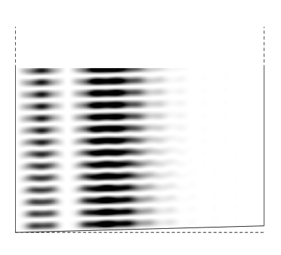
FIG. 2.: Density plot of $\left|\Psi_{55,2}(x,y)\right|^{2},$ the same state as in Fig. 1c. The state is shown in the lower quarter of the billiard, $y<0.25,$ and the scale is expanded in the $y$ direction by a factor 3 in order to show more details of the wave function. A dashed line is shown at $y=0.$

This smooth transition of the quantum levels contrasts with the mathematics of the classical periodic orbits used in the trace formula. With parallel sides to the billiard, there is a set of nonisolated periodic orbits contributing a very large term to the trace formula. An arbitrarily small slope mathematically eliminates all such nonisolated periodic orbits. However, for a bounce or two, they remain close to the ideal periodic orbits of the channel with two parallel sides.

Reference[8] sorts this out with respect to the trace formula. It is remarkable that the eigenstates and energies start to be substantially modified when $\epsilon\geq\left(R/an\pi\right)^{2}$ while the low terms of the trace formula and thus the so-called length spectrum, are only modified if $\epsilon\geq R/an\pi.$ In other words, the low terms of the trace formula are essentially unmodified if the actual billiard is a ideal stadium billiard with ‘optically flat’ errors much smaller than a wavelength. This is however, not good enough to guarantee that the wavefunctions are close to the ideal wavefunctions.

IV Bogomolny operator

The preceding results can be obtained by a method[5] based on Bogomolny’s[3] quasiclassical surface of section transfer operator, $T$. The main idea is to organize the phases which appear in the transfer operator and its eigenfunctions according to their rate of change as a function of position on the surface of section. Thus, there are ‘fast’ and ‘slow’ parts to the Bogomolny equation.

In the trapezoid problem above, we take the space part of the surface of section to be $y=1.$ The SSTO for billiards is

$$T(x,x^{\prime}|k)=\sqrt{\frac{1}{2\pi i\hbar}\left|\frac{\partial^{2}S(x,x^{\prime})}{\partial x\partial x^{\prime}}\right|}e^{i\frac{S(x,x^{\prime})}{\hbar}}.$$ (9)

Here the action, $S(x,x^{\prime})=\hbar kL(x,x^{\prime})$, is that of the classical orbit leaving the surface of section at $x^{\prime}$ and returning to it for the first time at $x.$ It is expressed by $L(x,x^{\prime}),$ the length of this path. The wavenumber $k$ $=$ $\sqrt{E}$ in our units. We focus on orbits in the neighborhood of the $(1,0)$ resonance orbits of the unperturbed square. Such an orbit starts at ${\bf r}^{\prime}{\bf=(}x^{\prime},1)$ and returns to ${\bf r}=(x,1)$ after making one bounce from the bottom at approximately ${\bf\bar{r}=}\left(\frac{1}{2}(x+x^{\prime}),\frac{1}{2}\epsilon(x+x^{\prime})\right)$. For small $x-x^{\prime},$ $L\approx 2+\frac{1}{4}(x-x^{\prime})^{2}-\epsilon(x+x^{\prime}).$

The second term of $kL$ is rapidly varying with $x^{\prime}$, the last term is relatively slow. We solve Eq. (1), i. e. $\int dx^{\prime}T(x,x^{\prime}|k)\psi(x^{\prime})=\psi(x),$ by making the Ansatz $\psi(x^{\prime})=\exp\left[\pm ik\sqrt{\epsilon}F(x^{\prime})\right]$. This function, which has an intermediate rate of variation, followed by stationary phase approximation for the integral, causes the important values of $x^{\prime}$ to be close to $x,$ and allows $F(x^{\prime})\approx F(x)+(x^{\prime}-x)f(x).$ Solution of Eq. (1) requires $k\sqrt{\epsilon}F=\frac{2}{3}\left[z_{m}-\alpha x\right]^{3/2},$ where $\alpha$ is defined in the previous section. This gives for $\psi$ the WKB approximation to the Airy function.

In short, the simplest version of this SSTO technique gives quasiclassically the same $\psi$ as the BOA. Knowing $\psi,$ the full wave function is given by $\Psi({\bf r)=}\int dxG_{0}\left[{\bf r,r(}x)\right]\psi(x),$ where the kernel $G_{0}$ is related to the free space Green’s function between a point ${\bf r}$ in the interior of the billiard and the point ${\bf r(}x)$ on the surface of section. The result is essentially the BOA.

Note that the SSTO gives first the surface of section wavefunction, then the BOA wavefunction, reversing the order of the Born-Oppenheimer approximation. The BOA is simpler and more intuitive, when it works.

V Diagonal states

We next give a result for which we cannot construct a simple BOA Ansatz. Consider the same trapezoidal billiard but now look for special states related to the $(1,1)$ periodic orbits of the square. Then, it’s not too hard to work out the SSTO by making the Ansatz $\psi(x^{\prime})=\exp(\pm ikx^{\prime}/\sqrt{2})\exp\left[\pm ik\sqrt{\epsilon}F(x^{\prime})\right]$. The first phase factor chooses orbits at approximately 45^∘ to the square sides. In this case, the result is that there are states, induced by the small perturbation, that are concentrated along the diagonal $(0,0)\rightarrow(1,1)$ but not along $(0,1)\rightarrow(1,0)$. [In an appropriate parameter range, we do expect states with ‘scars’ along that diagonal, however.] Such a state, obtained numerically, is shown in Figs. 3 and 4. We have found the 2-dimensional state $\Psi(x,y)$ to order $\epsilon,$ but it is too cumbersome to display here. The following wave function (for even $n$) vanishes on the boundary, and is the same as our theoretical wave function to order $\epsilon^{0}$ (but not $\epsilon$). It is not an adequate BOA Ansatz but it is simple and it gives the gross features of the result. The function is $\Psi(x,y)\approx\cos\left[\frac{1}{2}n\pi(x+\tilde{y})\right]u(x-\tilde{y})-\cos\left[\frac{1}{2}n\pi(x-\tilde{y})\right]u(x+\tilde{y})$ where $u(x)=\mathop{\rm Ai}(\alpha\left|x\right|-z_{0})$ for $\left|x\right|\leq 1$, extended with period two outside this range, and $\tilde{y}=(y-\epsilon x)/(1-\epsilon x)$. Here $z_{0}\approx 1.02$ is the first maximum of the Airy function. The energies of such states are given by $E_{n,m}=\frac{1}{2}\left(n\pi\right)^{2}+\frac{1}{2}\alpha^{2}z_{m}$ where $z_{m}$ is a zero or extremum of the Airy function. We display the remarkable nodal structure of such a state in Fig. 5.

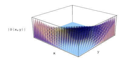
FIG. 3.: A three-dimensional representation of a state of the trapezoid concentrated near the long diagonal. The theoretical state is plotted. $\epsilon=0.03,$ $n=50,$ $m=0.$

With a little practice, it is easy to foresee when special states exist or not. For example, there are no states concentrated along the diagonal for the symmetric trapezoid billiard with sides $x=0,1$, $y=\epsilon x,$ $1-\epsilon x$, but there are states concentrated along the side $x=0$. For the parallelogram billiard with sides $x=0,1$, $y=\epsilon x$, $y=1+\epsilon x$, there are states along the long diagonal but no states near the edges.

VI Extended zone scheme

The BOA requires a choice of fast and slow variables. In the preceding example, a reflection of the wave incident on a boundary at 45^∘ switches the roles of $x$ and $y.$ The following device overcomes this difficulty, although it is cumbersome to apply to the example of the preceding section.

Consider a perturbed rectangular billiard. The perturbation can be a potential, a magnetic field, or magnetic flux lines. We assume the perturbation is classically weak, meaning that the classical orbit does not change much because of the perturbation in one traversal of the system. Our SSTO technique automatically gives the result[22], where pictures of some special states may be found.

For the BOA, we choose the important example where a magnetic field perturbs the $(1,1)$ resonance of the rectangle. First, we consider an auxiliary problem, a method of images, from whose solutions the desired answer is constructed.

The auxiliary problem extends the domain of the wavefunction to all of two dimensional space. The perturbing magnetic flux, originally defined only in the rectangle, is reflected about each of the sides of the rectangle, and then the process is repeated so that the result forms a lattice of period $2a$ in the $x$-direction, and period $2b$ in the $y$-direction. The vector potential is chosen to have this periodic structure.

FIG. 4.: The same state as shown in Fig. 3. The numerically obtained state is plotted, basically along the diagonals of the trapezoid. a) $\Psi(x,x)$, b) $\Psi(x,1-x).$ Also shown in part b) is the theoretical wavefunction, which is smoother. Part b) is plotted for $0<x<1/(1+\epsilon).$

Next we find the high energy wavefunctions of a periodic lattice, where the lattice potential is classically weak. The methods developed in the study of channelling[23] are appropriate and are effectively the BOA. We start with the $(1,1)$ channel, which amounts to assuming that the fast direction is given by the variable $\xi=(ax+by)/c$ and the slow by $\eta=(bx-ay)/c$, where $c=\sqrt{a^{2}+b^{2}}$. Take charge $e=1$, mass = $\frac{1}{2}$, and $\hbar=1$ and rewrite Schrödinger’s equation in variables $\xi$, $\eta$ as

$$\left\{\left[-i\partial_{\xi}-A_{\xi}(\xi,\eta)\right]^{2}+\left[-i\partial_{\eta}-A_{\eta}(\xi,\eta)\right]^{2}\right\}\Psi(\xi,\eta)$$ (10)

$$= E\Psi(\xi,\eta).$$ (11)

The channelling approximation averages along the fast, $\xi,$ direction. This amounts to assuming $\Phi(\xi|\eta)=\exp(ik\xi)$ and replacing $A_{\xi}(\xi,\eta)$ by $\bar{A}_{\xi}(\eta)=\int_{0}^{L_{\xi}}d\xi A_{\xi}(\xi,\eta)/L_{\xi}.$ Here $L_{\xi}=2c$. Because $k=-i\partial_{\xi}$ is large, the terms $A_{\xi,}^{2}$ $A_{\eta}^{2}$ can be neglected in comparison to $k\bar{A}_{\xi}(\eta)\$and $\bar{A}_{\eta}$ vanishes. The remaining $\eta$ dependence is obviously periodic.

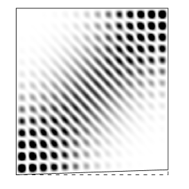
FIG. 5.: A density plot of a state similar to that shown in Figs. 3,4, with $n=28.$ The dashed line is $y=0.$

Take the origin at the rectangle center, for symmetry reasons. Let $\psi(\eta)=u(c\eta/b-a/2)=u(x-ay/b-a/2)$. Then $u$ satisfies

$$-u_{m}^{\prime\prime}(x)+V(x)u_{m}(x)=E_{m}u_{m}(x)$$ (12)

where

$$V(x)=-2{\textstyle{b^{2}\over c^{2}}}k\bar{A}_{\xi}\left({\textstyle{bx\over c}}+{\textstyle{ab\over 2c}}\right).$$ (13)

The reason for the shift in the definition of $u$ is that then $V(x)=V(-x)$, and $u$ will be simple on the boundaries where the Dirichlet conditions are imposed.

The integral defining $\bar{A}_{\xi}$ is the flux enclosed by the periodic orbit in the original rectangle, and so is independent of gauge. For uniform field $B$, $\bar{A}_{\xi}(\eta)=+B\eta(1-c\eta/ab)$ for $0\leq\eta<ab/c$, $\bar{A}_{\xi}(\eta)=-B(2ab/c-\eta)(c\eta/ab-1)$ for $ab/c\leq\eta<2ab/c$, $\bar{A}_{\xi}(\eta+2ab/c)=\bar{A}_{\xi}(\eta).$ In terms of $x$, $V(x)=-(Bkb^{3}a/c^{3})\left[\frac{1}{2}-2(x/a)^{2}\right]$ for $\left|x\right|<\frac{1}{2}a$,  repeated antiperiodically outside this region. The solution of Eq. (12) is a Bloch state, which satisfies

$$u_{m}(x+2a)=e^{i\beta}u_{m}(x),$$ (14)

where $m$ labels the ‘band’ and $\beta$, the ‘crystal momentum’. The band index $m$ is a quantum number and $\beta$ is yet to be determined. The energy is given by

$$E=k^{2}+c^{2}E_{m}/b^{2}.$$ (15)

Quantum states will be strongly affected by the flux if the dimensionless parameter $Bk(ab/c)^{3}$ is large. This parameter is $2\pi(\phi/\phi_{0})(kc)\left(ab/c^{2}\right)^{2}$, where $\phi$ is the flux $\phi=abB$, and $\phi_{0}=2\pi\hbar/e$ is the flux quantum.

We therefore find a set of approximate solutions to the plane problem, labeled by $k,\,m$ and $\beta$, $\Psi_{I}(x,y)=\exp\left[ik(ax+by)/c\right]u_{m}(x-ay/b-a/2)$. Given $\Psi_{I},$ another solution is given by the symmetry under rotation by $\pi$, $\Psi_{III}(x,y)=\Psi_{I}(-x,-y)$. Two other solutions are given by $\Psi_{II}(x,y)=\exp\left[ik(-ax+by)/c\right]u_{m}(-x-ay/b+a/2)$ and $\Psi_{IV}(x,y)=\Psi_{II}(-x,-y)$. All four of these channels clearly have the same energy.

The solution for the original rectangle can be constructed from these four solutions, provided some quantization conditions are met. We consider two subspaces, $r=\pm 1$, even or odd under $(x,y)\rightarrow(-x,-y).$ The state can be written in the form

$$\Psi_{nm}=A\left(\Psi_{I}+r\Psi_{III}\right)+B(\Psi_{II}+r\Psi_{IV}).$$ (16)

Imposing the condition $\Psi_{nm}\left(\pm\frac{1}{2}a,y\right)=0$ yields $A=-B\exp(-i\chi_{a})$, and $\exp(i\beta)=\exp(-2i\chi_{a})$ where $\chi_{a}=ka^{2}/c.$ The condition $\Psi_{nm}\left(x,\pm\frac{1}{2}b\right)=0$ gives $A=-rB\exp(i\chi_{b})$ and $\exp(i\beta)=\exp(2i\chi_{b})$ where $\chi_{b}=kb^{2}/c.$ Therefore, $\chi_{a}+\chi_{b}=\pi n$, where $n$ is even for $r=1,$ and odd for $r=-1.$ This yields

$$k=\frac{\pi n}{c}.$$ (17)

One finds $\beta=2\chi_{b}-2\pi n_{b}=-2\chi_{a}+2\pi n_{a}.$ We may assume that $\left|\beta\right|\leq\pi,$ which fixes the integers $n_{a,b}$ as the integer part of $\left(\chi_{a,b}\pi^{-1}+1/2\right)$. Then $n_{a}+n_{b}=ck/\pi=n.$

For a square, $a=b$, there is a further symmetry, and $\beta$ is either $0$ or $\pi,$ that is, the appropriate state is either at the band top or band bottom. For an arbitrary ratio $a/b$, $k\xi=k(ax+by)/c$ is not of the form $\pi n_{a}x/a+\pi n_{b}y/b.$ However, the $n_{a,b}$ just found are the integers which most closely satisfy this relation.

Another case of great interest is that of an Aharonov-Bohm flux line in an integrable billiard[24]. We show in Fig. 6 current streamlines of a state for the case of a unit square, $a=b=1,$ with a flux line at its center. The potential is this case is $V(x)=-C,$ $\left|x\right|<\frac{1}{2},$ $V(x)=+C,$ $\left|x-1\right|<\frac{1}{2},$ repeated with period $2.$ Here $C=$ $\left(2\pi\phi/\phi_{0}\right)k/\sqrt{8}$. In Fig. 6 we have taken $\phi/\phi_{0}=$ $0.1$, the flux in units of the flux quantum, to be small in order to minimize diffraction effects. The state is not much localized spatially, but the current is very regular. For symmetry reasons, the structure is particularly simple along a coordinate axis, as we display in the figure. Because of diffraction, our theory of the flux line case has relatively large corrections. Nevertheless, our simple theory captures the main features of many states. We have related results[25] published elsewhere.

In this case of a perturbed rectangular billiard, we have been able to find a bigger problem which admits a decomposition into fast and slow variables and thus a Born-Oppenheimer Ansatz. The original problem is solved by a superposition of results of the auxiliary problem.

VII Fast and slow asymptotics

We now give an example in which a separation of variables into fast and slow does not hold over the whole domain, but does work over a limited domain, that is, however, sufficient to solve the problem.

Consider a weakly distorted unit circle billiard. This is defined in polar coordinates by the boundary $r=1+\epsilon\Delta R(\theta)$, where $\epsilon$ is small, $\Delta R\,$ is of order unity, and $\Delta R$ does not vary too rapidly. A number of papers have appeared on this topic recently[6].

FIG. 6.: Upper figure: Numerical persistent current streamlines of a state induced by an Aharonov-Bohm flux line containing 0.1 flux quanta, located at the center of a square billiard. A quarter of the billiard is shown. Lower figure: Current in the $y$-direction on the $y$ axis. The theoretical current is plotted. The numerical current is similar but has minima at the depths shown by the horizontal lines. The quantum numbers are $n=82,$ $m=0.$

We confine attention to high energy states whose classical counterparts pass close to the center of the billiard. Such states have low angular momentum, that is, dimensionless angular momenta $\nu<<k$. This suggests that we consider the radial variable $r\,$ to be ‘fast’, and the angular variable $\theta$ to be ‘slow’ and thus the Ansatz $\Phi=J_{\nu(\theta)}(kr)$. This, however, does not work. The reason is that near the origin, $r$ is not fast compared with $\theta.$

However, we need to know $\Phi$ only near the boundary in order to impose the Dirichlet conditions. Without a condition at the origin, using the asymptotic expansion for Bessel’s functions suggests the Ansatz

$$\Phi(r|\theta)\approx\frac{1}{\sqrt{kr}}\cos\left[kr+\frac{\nu(\theta)^{2}-\frac{1}{4}}{2kr}+\alpha(\theta)\right]$$ (18)

where $\nu(\theta)$ is the order of the Bessel functions and $\alpha(\theta)$ is a phase which mixes the asymptotic Bessel and Neumann functions. The slow equation is $\psi^{\prime\prime}+\nu^{2}\psi=0.$ To make $\Phi$ vanish at $r=1+\epsilon\Delta R(\theta)$ requires

$$k+k\epsilon\Delta R(\theta)+\frac{\nu(\theta)^{2}-\frac{1}{4}}{2k}+\alpha(\theta)=(n-\frac{1}{2})\pi.$$ (19)

It is necessary to determine two functions, $\nu$ and $\alpha$, from Eq. (19). We expect $\nu$ to depend on $\frac{1}{2}\left[\Delta R(\theta)+\Delta R(\theta\pm\pi)\right]\equiv\overline{\Delta R(\theta)}$, and not on $\delta R(\theta)\equiv\frac{1}{2}\left[\Delta R(\theta)-\Delta R(\theta\pm\pi)\right].$ Classically, a low angular momentum state sees equally both sides of the circle, if at $\theta,$ then also at $\theta\pm\pi.$ To achieve this, we take $\alpha(\theta)=-k\epsilon\delta R(\theta)+\alpha_{0},$ where $\alpha_{0}$ is to be determined. This implies that

$$\nu(\theta)^{2}=E_{m}-V(\theta)$$ (20)

where $V(\theta)=2k^{2}\epsilon\overline{\Delta R(\theta)}.$ This acts as a potential in the slow equation, and it will be important if $k\sqrt{\epsilon}>>1.$

Again there is a Schrödinger equation with a periodic potential $V(\theta)=V(\theta+\pi),$ and thus solutions labelled by the band index $m$ and ‘crystal momentum’ $\beta.$ Since physically $\psi(\theta+2\pi)=\psi(\theta)$, $\beta=0$ or $\pi.$ The constant $\alpha_{0}$ is determined from the special case $\Delta R=0,$ which implies $E_{m}=m^{2},$ with $m$ integer, $\beta=\pi\left(m\mathop{\rm mod}2\right).$ For $\Delta R=0,$ the solution $\Phi(r|\theta)=J_{m}(kr)$ implies $\alpha_{0}=\frac{1}{2}\beta-\pi/4.$

In Fig. 7 we show a state for a stadium billiard as in Sec. III, with a short straight side of length $2a=2\epsilon=0.02$ and end radius $R=1.$ Then $\Delta R=\epsilon\left|\cos\theta\right|+O(\epsilon^{2}).$ Some other states are shown in Ref.[5].

FIG. 7.: Numerically obtained contour plot of a state of a Bunimovitch stadium billiard with end cap radius unity.whose straight sides are short, of length $2a,$ where $a=0.01.$ The parallel lines near the left side of the boundary have separation $2a.$ This state has $m=3,$ i.e. two transverse nodes, and $n=25.$

This application of the BOA differs from others in that we do not have a separation into slow and fast variables over the whole system, but we do have such a separation, asymptotically, over the part of the system that matters most.

VIII Whispering gallery modes

Quantization of higher order periodic orbit resonances in nearly circular billiards cannot be done easily by a Born-Oppenheimer method. However, the whispering gallery limit can be handled with a modification of the BOA, and is not restricted to the nearly circular case. Rather, we assume only a two dimensional smooth convex billiard.

The results have long been known, but the methods we introduce are easier and more intuitive than earlier techniques. These modes correspond to classical motion which stays close to the billiard boundary while rapidly moving along the boundary. The effect was discussed by Lord Rayleigh, first for rays in his Theory of Sound, and later in terms of waves[11]. Lord Rayleigh did not consider the eigenmodes, however, which were first quantized by Keller[14] as an example of what came to be known as EBK quantization. Keller’s work was based on the assumption of the existence of caustics in the corresponding classical motion. This was proved later by Lazutkin[26] who obtained an adiabatic invariant.

We first obtain the result by SSTO. The surface of section is the billiard boundary. Let $s$ be the distance along the boundary. The ray goes from $s^{\prime}$ to $s,$ with $s^{*}=s-s^{\prime}$ small.

Let the radius of curvature at $\bar{s}=\frac{1}{2}(s+s^{\prime})$ be $R(\bar{s}).$ The curvature varies slowly in the sense $dR/d\bar{s}$ never gets too large and $R$ is always positive and finite. Then, we use Eq. (9) above and approximate

$$L(s,s^{\prime})\simeq 2R(\bar{s})\sin\frac{1}{2}\left|\frac{s-s^{\prime}}{R(\bar{s})}\right|\approx\left|s-s^{\prime}\right|-\frac{\left|s-s^{\prime}\right|^{3}}{24R(\bar{s})^{2}}.$$ (21)

We now look for a solution of Eq. (1).   We take as Ansatz

$$\psi(s)=\exp\left\{ik\left[s-F(s)\right]\right\}$$ (22)

where $dF/ds\equiv f(s)<<1.$ Thus, apart from the explicit $\exp(iks)$, $\psi(s)$ varies relatively slowly.

We do the integral $T\psi$ by stationary phase. [The BOA below improves on this.] The stationary phase point is $s^{\prime}=s-s^{*}$ where $\left(s^{*}\right)^{2}/8R^{2}=f$. It can be checked later that the $s^{\prime}$ dependence of $R$ can be neglected. Doing the integral gives

$$T\psi=i\exp\left[i\frac{2}{3}kR(2f)^{3/2}\right]\psi(s).$$ (23)

A solution requires

$$f=f_{m}(s)=F_{m}^{\prime}=\left[\frac{3\pi}{\sqrt{8}kR(s)}(m+\frac{3}{4})\right]^{\frac{2}{3}}.$$ (24)

This is the first quantization condition. The condition that $f$ be small requires  $m<<kR(s).$

The other quantization condition is a result of the requirement that $\psi$ is single valued on the boundary, that is, $\psi(0)=\psi({\cal L})$ where ${\cal L}$ is the circumference of the billiard. This condition can be expressed

$$k\left[{\cal L}-F_{m}({\cal L})+F_{m}(0)\right]=2\pi n$$ (25)

Thus the quantization depends on $\int_{0}^{{\cal L}}R(s)^{-2/3}ds,$ effectively the mean 2/3 power of the curvature.

We now turn to the BOA. The billiard is locally a circle of radius $R(s).$ If $R$ is constant, the solution is $\Psi=J_{\nu}(kr)e^{i\nu\theta}$ where $J_{\nu}$ is a Bessel function. We assume $\nu$ is large. [This is close to the treatment of Lord Rayleigh, who, however, takes for granted that the index $\nu$ is an integer. Most of the rest of his discussion concerns the asymptotic properties of Bessel functions of large index, a subject still under development at the time. The etalon method also considers this Bessel function, but does not distinguish fast and slow variables.]

We assume that for a more general convex billiard $\Psi$ has this form locally. Namely we make the Ansatz

$$\Psi({\bf r})=\Phi(\rho|s)\psi(s)=J_{\nu(s)}(kr_{s})\psi(s)$$ (26)

where $r_{s}$ is a radial coordinate from the local center of curvature. Let the variable $\rho\geq 0$ be given by $r_{s}=R(s)-\rho.$ With the exception of the factor $\exp(iks)$ all $s$ dependence is slow compared with the ‘fast’ variable $\rho.$ The index $\nu$ can vary smoothly and there is no reason to make it an integer. We could already guess $\psi(s)=\exp\left[i\int^{s}d\bar{s}\,\nu(\bar{s})/R(\bar{s})\right]$ where we have replaced the local angle variable $d\theta_{s}$ by $ds/R.$ Parametrize $\nu=kR(1-f)$ where $f$ is small (and turns out to be the same $f$ introduced earlier). Using a standard asymptotic formula[27] we have

$$J_{\nu(s)}\left(k\left[R(s)-\rho\right]\right) = J_{\nu}\left[\nu+\nu^{\frac{1}{3}}\left(\frac{kRf-k\rho}{\nu^{\frac{1}{3}}}\right)\right]$$ (27)

$$\simeq \left(\frac{2}{kR}\right)^{\frac{1}{3}}\mathop{\rm Ai}\left[-2^{\frac{1}{3}}\frac{kRf-k\rho}{\left(kR\right)^{\frac{1}{3}}}\right].$$ (28)

We can replace $\nu^{1/3}$ by $(kR)^{1/3}$ when multiplied with the small quantities $f$ or $\rho.$

The first quantization condition is that $\nu(s)$ must be chosen to solve $J_{\nu(s)}\left[kR(s)\right]=0.$ A convenient analytic approximation is obtained from Eq. (28), again in terms of the zeroes $z_{m}$ of the Airy function,

$$f=z_{m}/2^{\frac{1}{3}}(kR)^{\frac{2}{3}}.$$ (29)

This improves on Keller’s treatment or the $T$ operator above which is equivalent to approximating $\mathop{\rm Ai}(-x)\propto\sin(\frac{2}{3}x^{\frac{3}{2}}+\frac{\pi}{4}),$ valid for large $x.$

To find $\psi(s)$ we substitute the Ansatz of Eq. (26) into the Helmholtz equation, neglecting derivatives of $J_{\nu}$ with respect to $s.$ The angular derivative term $(1/r_{s})^{2}\partial^{2}/\partial\theta_{s}^{2}$ can be replaced by $\partial^{2}/\partial s^{2}$ so we see that $\psi^{\prime\prime}(s)+(\nu^{2}/R^{2})\psi=0.$ This has the approximate solution given in Eq. (22) above. From this, the requirement that the wavefunction be single valued on the boundary gives the second quantization condition. Thus the solution is

$$\Psi(s,\rho)\approx C(s)\mathop{\rm Ai}\left(-z_{m}+\frac{k\rho}{\left[kR(s)\right]^{\frac{1}{3}}}\right)\psi(s)$$ (30)

The slowly varying prefactor $C(s)$ is a normalization of the Airy function determined by current conservation.

The validity of the BOA requires that the argument of the Airy function vary more rapidly with $\rho$ than with $s$ [in the region that the Airy function is large]. This condition can be written $\left|R^{\prime}\right|<<\left(kR\right)^{2/3}/z_{m}.$ The existence of a classical constant replacing $k^{2/3}/z_{m}$ in this strong inequality is the condition for the existence of a caustic. The caustic is at the zero argument of the Airy function, i.e. at $\rho=z_{m}(kR)^{1/3}/k.$ Thus if $R$ is finite and smooth, there is always a sufficiently large energy such that states remaining close to the boundary exist.

If $1/R$ vanishes at some point, it is known that caustics do not exist, and the BOA must fail near that point. However, numerical evidence (at relatively low energies, of course) suggests that whispering gallery states exist even when the curvature vanishes. No detailed theory has been advanced for this case, to our knowledge. We have made some progress on this problem, which will be published elsewhere.

IX Conclusions

With slight extensions, the Born-Oppenheimer approximation can, rather quickly and easily, give the leading order results for a number of interesting states. These include the important and well-known cases of the whispering gallery modes, and the bouncing ball states. It also includes some states only recently uncovered by the SSTO method. It is relatively easy to apply when, at least asymptotically, the variables can be separated into fast and slow. This can happen because of a small parameter, or just because the particular state has that special property.

The PEM and etalon methods are similar to the BOA in the sense that they deal directly with the partial differential equations. The detailed procedures and motivations for each step is rather different from the BOA. The leading results are the same, however. An advantage of the BOA is that it is simpler and taught in standard courses on quantum mechanics while the other methods are less well known.

These methods are not a priori semiclassical. However, if a variable is fast because it has more energy than the slow variable, semiclassical methods can be used. The Keller-Rubinow method is classic, but a little cumbersome in practice. The SSTO method seems to be in a certain sense more general than the Born-Oppenheimer. Compared with Keller-Rubinow, it has the advantage of the simplifications coming from use of the surface of section. Compared with BOA, it first finds the slow wavefunction, and from that the fast one. Often the slow wavefunction is more interesting physically.

Another well known semiclassical method sometimes compared with the SSTO method is the Birkhoff-Gustavson normal form[28]. However, Birkhoff-Gustavson is not adapted to finding special wavefunctions. It rather gives a large number of wavefunctions and energy levels at once, and is similar to a numerical method in that respect.

Formal corrections to the PEM and etalon methods have been written down[17], which differ from the usual methods used with the BOA. These corrections are not much used in practice. Rather, one resorts to a numerical method. Moreover, quite large corrections to the wavefunctions are sometimes found in the numerics. This is because the theory singles out some relatively small subset of special states which are approximately decoupled from all the rest. Nothing prevents some unrelated state from having nearly the same energy as the special state. The residual coupling then mixes the two appreciably. The energies are given quite well, although not necessarily as accurately as the mean level spacing of all the levels.

Although it is sometimes possible to find approximations to both states and to estimate the mixing parameters, it is hard to do that systematically. It is perhaps more advisable to think of the wavefunctions obtained as being those of quasimodes[29], in other words, as linear superpositions of a few nearly degenerate true eigenstates. In many situations, of course, a quasimode provides a correct and more physical description of a phenomenon than the true eigenmodes.

X Acknowledgments

Supported in part by the United States NSF grant DMR-9625549 and United States-Israel Binational Science Foundation, grant 99800319. R.N. was partially supported by the NSF grant DMR98-70681 and the University of Kentucky. We thank Prof. Director Peter Fulde for hospitality at the Max-Planck-Institut für Physik komplexer Systeme in Dresden, where some of this work was done.

REFERENCES

- [1] M. C. Gutzwiller, J. Math. Phys. 12, 343 (1971); Chaos in Classical and Quantum Mechanics, (Springer-Verlag, New York, 1990).
- [2] A. Voros, J. Phys. A21, 685 (1988); P. Cvitanović and B. Eckhardt, Phys. Rev. Lett. 63, 823 (1989); M. V. Berry and J. P. Keating, Proc. R. Soc. London, Ser. A 437, 151 (1992); E. Doron and U. Smilansky, Phys. Rev. Lett. 68, 1255 (1992).
- [3] E. B. Bogomolny, Nonlinearity 5, 805 (1992), and references therein.
- [4] R. Blümel, et. al., Phys. Rev. E 53, 3284 (1996).
- [5] R. E. Prange, R. Narevich, and O. Zaitsev, Phys. Rev. E 59, 1694 (1999).
- [6] F. Borgonovi, et al, Phys. Rev. Lett. 77, 4744 (1996); J. U. Nöckel and A. D. Stone, Nature 385, 45 (1997); K. M. Frahm and D. M. Shepelyansky, Phys. Rev. Lett. 78, 1440 (1997); ibid. 79, 1833 (1997); F. Borgonovi, Phys. Rev. Lett. 80, 4653 (1998).
- [7] K. Richter, D.Ullmo, and R. A. Jalabert, Phys. Reports 276, 1 (1996); K. Richter, Habilitationsschrift der Universität Augsburg (Max-Planck-Institut, Dresden, 1997); M. Brack and R. K. Bhaduri, Semiclassical Physics (Addison-Wesley, Reading, 1997).
- [8] H. Primack and U. Smilansky, J. Phys. A: Math. Gen. 27, 4439 (1994).
- [9] L. Kaplan and E. J. Heller, Physica D 121, 1 (1998).
- [10] M. Born and J. R. Oppenheimer, Ann. Phys. (Leipzig) 84, 457 (1927).
- [11] Lord Rayleigh, Phil. Mag. 27, 100 (1914).
- [12] C. Dembowski, et. al., Phys. Rev. Lett. 84, 867 (2000).
- [13] A. Wallraff, et. al., Phys. Rev. Lett. 84, 151 (2000).
- [14] J. B. Keller and S. I. Rubinow, Ann. Phys. (New York) 9, 24 (1960).
- [15] M. A. Leontovich, Izv. Akad. Nauk SSSR, Ser. Fiz. 8, 16 (1944).
- [16] V. A. Fock, Izv. Akad. Nauk SSSR, Ser. Fiz. 10(2), 171 (1946) [J. Phys. USSR 10, 399 (1946)]; Electromagnetic Diffraction and Propagation Problems, 2nd ed. (Sovetskoe Radio, Moscow, 1970) [1st ed. (Pergamon, Oxford, 1965)].
- [17] V. M. Babich and V. S. Buldyrev, Short Wavelength Diffraction Theory (Springer-Verlag, Berlin, 1991).
- [18] For example, G. Baym, Lectures on Quantum Mechanics (W.A. Benjamin, New York, 1969); A. Messiah, Quantum Mechanics, Vol. II (Wiley, New York, 1966).
- [19] P. M. Morse and H. Feshbach, Methods of Theoretical Physics, Vol. II (McGraw-Hill, New York, 1953).
- [20] Y. Y. Bai, et al, Phys. Rev. A 31, 2821 (1985).
- [21] S. W. McDonald, Ph. D. Thesis (Berkeley, 1983).
- [22] R. Narevich, R. E. Prange, and O. Zaitsev, Phys. Rev. E 62, 2046 (2000).
- [23] J. Lindhard, Dan. Mat. Fys. Medd. 34(14) (1965).
- [24] M. Sieber, Phys. Rev. E 60, 3982 (1999); E. Bogomolny, N. Pavloff and C. Schmit, Phys. Rev. E 61, 3689-3711 (2000); S. Rahav and S. Fishman (to be published, this issue).
- [25] R. Narevich, R. E. Prange and Oleg Zaitsev, Physica E (to be published).
- [26] V. F. Lazutkin, KAM Theory and Semiclassical Approximations to Eigenfunctions (Springer-Verlag, Berlin-Heidelberg, 1993).
- [27] Handbook of Mathematical Functions, edited by M. Abramowitz and I. Stegun (Dover, N.Y., 1965).
- [28] G. D. Birkhoff, Dynamical Systems (Am. Math. Soc., New York, 1966), Vol. IX; F. G. Gustavson, Astron. J. 71, 670, (1966).
- [29] V. I. Arnol’d, Funktional. Anal. i Prilozen. 6, 12 (1972) [Functional Anal. Appl. 6, 94 (1972)].