Stability and instability of a hot and dilute nuclear droplet

Abstract

The diabatic approach to collective nuclear motion is reformulated in the local-density approximation in order to treat the normal modes of a spherical nuclear droplet analytically. In a first application the adiabatic isoscalar modes are studied and results for the eigenvalues of compressional (bulk) and pure surface modes are presented as function of density and temperature inside the droplet, as well as for different mass numbers and for soft and stiff equations of state. We find that the region of bulk instabilities (spinodal regime) is substantially smaller for nuclear droplets than for infinite nuclear matter. For small densities below 30% of normal nuclear matter density and for temperatures below 5 MeV all relevant bulk modes become unstable with the same growth rates. The surface modes have a larger spinodal region, reaching out to densities and temperatures way beyond the spinodal line for bulk instabilities. Essential experimental features of multifragmentation, like fragmentation temperatures and fragment-mass distributions (in particular the power-law behavior) are consistent with the instability properties of an expanding nuclear droplet, and hence with a dynamical fragmentation process within the spinodal regime of bulk and surface modes (spinodal decomposition).

1 Introduction and summary

In bombardments of nuclei with light and heavy ions, as well as by absorption of pions and antiprotons in nuclei, transient systems are produced at excitation energies around 10 MeV/u, which decay into several fragments of intermediate size. Increasing interest b1 ; b1* ; b2 ; b3 in this multifragmentation reaction has been initiated by the observation b4 that the fragment-mass distribution is proportional to $A^{-\sigma}$ (power law with $\sigma\approx 2.6$) indicating that the process may be related to the critical point of the liquid-gas phase transition of nuclear matter. Indeed, simulations within molecular dynamics b7 ; b6 ; b5 and mean-field approaches b8 ; b9 ; b10 ; b11 show that initial compression in central heavy-ion collisions or pure excitation of a nucleus by abrasion of nucleons or by absorption of light ions, pions or antiprotons cause the system to expand and to break up into pieces in a low-density regime. Power-law fragment-mass distributions have also been obtained from dynamical nucleation in a thermodynamically unstable nucleonic system b11* . However, as indicated by the great success of statistical models b12 ; b13 ; b14 ; b15 , the observables in multifragmentation seem to be mainly determined by the available phase space at the point of freeze out b17* . This conclusion remains valid even if the time evolution (expansion) of the statistically emitting source is taken into account b16 .

With the discovery of a caloric curve in projectile fragmentation by the ALADIN collaboration b17 , the nuclear liquid-gas phase transition as a mediator between the heated expanding nuclear matter and its decay into pieces moved again into the center of discussions. The growth of density instabilities within the spinodal region inside the phase coexisting regime, known as spinodal decomposition b18 , has early been considered as a possible mechanism of multifragmentation b19 ; b20 ; b21 . Extending Landau’s Fermi-liquid theory to finite temperatures Heiselberg, Pethick and Ravenhall b22 have investigated the stability and instability of hot and dilute infinite nuclear matter. Subsequent studies have been concerned with detailed properties of nuclear matter b23 and finite droplets b26 ; b25 ; b27 ; b24 in and around the spinodal regime. Quantal effects, as studied within constrained RPA b25 , do not alter the adiabatic instabilities as calculated from a fluid-dynamical description b26 and simulations b27 within a stochastic mean field approach. Some experimental evidence for spinodal decomposition has been reported by Rivet et al. b28 .

Our model for examining the stability and instability of a hot and dilute nuclear droplet is based on the diabatic approach to dissipative large-amplitude collective motion b29 ; b30 ; b31 and, by the use of a local energy-density approximation, is similar in spirit to the Fermi liquid-drop model of Kolomietz and Shlomo b24 . However, instead of using the fluid-dynamical approach with the boundary of zero total pressure on the fixed surface as in b24 ; b43 , we consider a general displacement field, which is defined by an expansion of the displacement potential in terms of multipoles, and include Coulomb interactions. This expansion with a suitable boundary condition for the complete basis set allows the analytical evaluation of collective mass and stiffness tensors within a consistent harmonic approximation. The set of eigenvalue equations couple modes with different number of nodes in the radial function of the displacement field. In contradistinction to b26 , where dispersion relations of the energy as function of radial wave number for different multipoles have been obtained in the adiabatic limit (no deformations of the local Fermi sphere), we determine the orthogonal eigenmodes of the droplet as function of the relaxation time $\tau$ for the decay of deformations of the local Fermi sphere, i.e. continuously from the adiabatic to the diabatic limit. Furthermore we study also pure surface modes and compare the instability properties for soft and stiff equations of state. In this way we extend the exploratory studies b26 ; b25 ; b27 ; b24 of spinodal instabilities of finite droplets to a more systematic analysis of stability and instability by examining the eigenmodes of a nuclear droplet as functions of densities and temperatures, relevant in the multifragmentation process.

In the following, which forms part I of a series of publications, we present detailed results on isoscalar bulk and surface modes with fixed ratio of neutron and proton densities in the adiabatic limit (very fast equilibration, $\tau\rightarrow 0$). Since $\tau\propto T^{-2}$, cf. b32 , this corresponds to the high-temperature limit. We have studied these adiabatic isoscalar modes in detail, because they are related to thermodynamics and to many studies performed in the past. In subsequent papers we will present the modifications due to dissipation ($0<\tau<\infty$) and extend the study to the inclusion of isovector modes, which to our knowledge have been studied so far only for infinite nuclear matter b33 ; b34 ; b37* and for a lattice gas b35 .

The results on adiabatic isoscalar bulk instabilities (preliminary calculations have been presented earlier b36 ) are summerized as follows.

• As compared to infinite nuclear matter the spinodal region for compressional (bulk) instabilities shrinks to smaller densities and temperatures with $T_{\mathrm{crit}}=6$ MeV for a soft equation of state (EOS). This effect is due to an increase of stability, which results from the Weizsäcker term $\propto(\vec{\nabla}\varrho)^{2}$ in the energy density and the finite wave lengths of density fluctuations in the droplet. The observed fragmentation temperatures of about 5 MeV (cf. b17 ) are consistent with spinodal decomposition after expansion. Typical values for the growth rates are $\gamma\approx 5$ MeV corresponding to growth times $\hbar/\gamma\approx 40$ fm/c.

• Effects from Coulomb interactions on the bulk instabilities are negligible, although, as shown in b37 , they are important at later stages of the multifragmentation process, where statistical models apply.

• As compared to the soft EOS, a stiff EOS yields a larger spinodal region with $T_{\mathrm{crit}}=8$ MeV. Typical values for the growth rates of instabilities are larger by almost a factor 2.

• With decreasing density and temperature the modes with the lowest multipolarities and no radial node become unstable first.

• At densities below $0.3\varrho_{0}$ (with $\varrho_{0}=0.16$ fm^-3) the instability growth rates for different multipolarities $(l=2,3,4,5)$ and number of nodes $(n=0,1,2,3)$ are practically equal. This property can yield a power-law behavior $A^{-\sigma}$ with $\sigma\approx 2.0$ of the fragment-mass distribution in agreement with experimental observations, cf. b38 and is not related to the critical point. Additional components from evaporation at lower excitation energies and non-equilibrium coalescence at higher excitation energies are considered responsible for the observed larger values of $\sigma$.

For finite nuclear droplets surface modes are important in addition to the compressional modes. Indeed, pure surface modes show some interesting features.

• The instability region of pure surface modes extends to larger densities up to about the spinodal line of infinite nuclear matter and to large temperatures.

• In general the growth times are smaller by half an order of magnitude as compared to the typical values for bulk instabilities.

• In the stable region surface modes are slow, such that deformations initiated in the excitation process will persist during expansion and clustering.

• The surface instability is dominated by quadrupole deformation. Fission at high excitation energies is expected to take this path through a low density stage, where the fission barrier vanishes. This is a novel mechanism of fission and may be even faster than the standard path across the barrier at equilibrium density.

In the following section 2 we introduce the collective model, which serves as the basis for our studies of stability and instability of nuclear droplets. In section 3 we describe the application to adiabatic isoscalar modes of compressional and pure surface deformations. Results on stability and instability of expanding nuclear droplets are presented in section 4. Relations to multifragmentation are discussed in section 5. Details of derivations and evaluations are given in the Appendix.

2 The collective model

We apply the diabatic approach to dissipative collective motion b29 ; b30 ; b31 . In contradistinction to adiabatic models, dynamical distortions of the Fermi sphere are included and dissipation due to two-body collisions give rise to a term in the collective equation of motion, which is non-local in time (non-markovian friction).

2.1 Reminder of the diabatic approach

If we introduce a set $\vec{g}\equiv\{g_{\lambda}\}$ of collective variables $g_{\lambda}(t)$ in the irrotational velocity field

$$\vec{v}(\vec{r},t)=\vec{\nabla}W(\vec{r},\vec{g},\dot{\vec{g}})=\sum_{\lambda}\dot{g}_{\lambda}\,\vec{\nabla}w_{\lambda}(\vec{r},\vec{g})$$ (1)

of collective motion, we can rigorously define (stationary) diabatic single-particle states $|\widetilde{\phi}_{\alpha}(\vec{g})\rangle$ by

$$\frac{\partial}{\partial g_{\lambda}}|\widetilde{\phi}_{\alpha}(\vec{g})\rangle=-\frac{1}{2}\{(\vec{\nabla}w_{\lambda})\cdot\vec{\nabla}+\vec{\nabla}\cdot(\vec{\nabla}w_{\lambda})\}|\widetilde{\phi}_{\alpha}(\vec{g})\rangle$$ (2)

i.e. by an infinitesimal unitary transformation, which deforms the wave function in accordance with the velocity field (cf. Appendix A). We search for the solution $|\Psi(t)\rangle$ of the many-body Schrödinger equation by expanding

$$|\Psi(t)\rangle=\sum_{\nu}c_{\nu}(t)\,|\Psi_{\nu}(\vec{g},\dot{\vec{g}},t)\rangle$$ (3)

in terms of Slater determinants $|\Psi_{\nu}\rangle$, which are built from the boosted diabatic single-particle states

$$|\widetilde{\psi}_{\alpha}\rangle\equiv\exp\left\{\frac{i}{\hbar}\left[m_{N}W(\vec{g},\dot{\vec{g}})-\int_{t_{0}}^{t}\mathrm{d}t^{\prime}\,\varepsilon_{\alpha}(t^{\prime})\right]\right\}|\widetilde{\phi}_{\alpha}(\vec{g})\rangle$$ (4)

moving with the velocity field $\vec{v}$. Here, $\varepsilon_{\alpha}$ and $m_{N}$ denote the diabatic single-particle energies and the nucleon mass, respectively.

From the variational principle

$$\delta_{c_{\nu},g_{\lambda}}\int_{t_{0}}^{t_{1}}\mathrm{d}t\,\langle\Psi(t)|i\hbar\frac{\partial}{\partial t}-H|\Psi(t)\rangle=0$$ (5)

with the many-body Hamiltonian $H$, one derives equations of motion for the expansion coefficients $c_{\nu}(t)$ and collective variables $g_{\lambda}(t)$. The coupled equations for the expansion coefficients describe the mixing of states (essentially due to residual interactions), and hence the equilibration process within the intrinsic degrees of freedom. We approximate this equilibration by a relaxation equation for the diabatic single-particle occupation probabilities

$$\frac{\mathrm{d}n_{\alpha}(t)}{\mathrm{d}t}=-\frac{1}{\tau(t)}\{n_{\alpha}(t)-\overline{n}_{\alpha}(\vec{g},\mu,T)\}$$ (6)

where $\tau$ and $\overline{n}_{\alpha}$, respectively, denote the relaxation time and the equilibrium values of the occupation probabilities. The chemical potential $\mu(t)$ and the temperature $T(t)$ in the Fermi distribution for $\overline{n}_{\alpha}$ are determined by the conservation of mass and excitation energy in the relaxation process. The relaxation time $\tau$ has been estimated for normal nuclear matter by several groups, cf. b39 , and given as

$$\frac{\tau}{\hbar}=\frac{\eta}{\varepsilon^{*}}$$ (7)

with values for $\eta$ between 0.15 and 0.30 depending on the magnitude of the nucleon-nucleon cross-section in medium.

The collective equation of motion, as obtained from the variation (5) with respect to $q_{\lambda}$, is given by b39*

$$\frac{\mathrm{d}}{\mathrm{d}t}\sum_{\lambda\lambda^{\prime}}\,B_{\lambda\lambda^{\prime}}\,\dot{g}_{\lambda^{\prime}}-\frac{1}{2}\sum_{\lambda^{\prime}\lambda^{\prime\prime}}\,\frac{\mathrm{d}B_{\lambda^{\prime}\lambda^{\prime\prime}}}{\mathrm{d}g_{\lambda}}\dot{g}_{\lambda^{\prime}}\dot{g}_{\lambda^{\prime\prime}}=F_{\lambda}\;,$$ (8)

where $B_{\lambda\lambda^{\prime}}$ denotes the collective mass tensor

$$B_{\lambda\lambda^{\prime}}=m_{N}\int\mathrm{d}^{3}r\,\widetilde{\varrho}(\vec{r})(\vec{\nabla}w_{\lambda})\cdot(\vec{\nabla}w_{\lambda^{\prime}})$$ (9)

for the velocity field (1) and the density

$$\widetilde{\varrho}(\vec{r})=\sum_{\alpha}n_{\alpha}|\widetilde{\phi}_{\alpha}(\vec{r})|^{2}\;.$$ (10)

The force on the r.h.s. of (8) is determined by

$$F_{\lambda}=-\sum_{\alpha}\frac{\partial\varepsilon_{\alpha}(\vec{g})}{\partial g_{\lambda}}\,n_{\alpha}(t)$$ (11)

in the diabatic representation. Note that the diabatic single-particle energies are smooth functions of $\vec{g}$ and that the force is defined for fixed $n_{\alpha}$, i.e. for constant (single-particle) entropy.

Inserting in (11) the formal integral of (6)

$$n_{\alpha}(t)=\overline{n}_{\alpha}(t)-\int_{t_{0}}^{t}\mathrm{d}t^{\prime}\,\frac{\mathrm{d}\overline{n}_{\alpha}}{\mathrm{d}t^{\prime}}\,e^{-\int_{t^{\prime}}^{t}\,\mathrm{d}t^{\prime\prime}/\tau(t^{\prime\prime})}$$ (12)

with the initial value $n_{\alpha}(t_{0})=\overline{n}_{\alpha}(t_{0})$, we obtain

$$F_{\lambda}(\vec{g},t)=\overline{F}_{\lambda}(\vec{g},t)+F^{\prime}_{\lambda}(\vec{g},t)\;,$$ (13)

$$\overline{F}_{\lambda}(\vec{g},t)=-\sum_{\alpha}\frac{\partial\varepsilon_{\alpha}(\vec{g})}{\partial g_{\lambda}}\,\overline{n}_{\alpha}\;,$$ (14)

$$F^{\prime}_{\lambda}(\vec{g},t)=\sum_{\alpha}\frac{\partial\varepsilon_{\alpha}(\vec{g})}{\partial g_{\lambda}}\int_{t_{0}}^{t}\mathrm{d}t^{\prime}\,\frac{\mathrm{d}\overline{n}_{\alpha}}{\mathrm{d}t^{\prime}}\,e^{-\int_{t^{\prime}}^{t}\,\mathrm{d}t^{\prime\prime}/\tau(t^{\prime\prime})}.$$ (15)

The equilibrium force is determined by the equilibrium distribution $\overline{n}_{\alpha}(t)$ for the time-dependent temperature and chemical potential. For temperatures ($T\approx 1$ MeV) large compared to the residual single-particle coupling, i.e. difference between the total mean field potential (adiabatic potential) and the diabatic potential, $\overline{F}_{\lambda}$ is identical to the adiabatic force, because the sum of neighboring energies is the same in both cases (invariance of trace). The elastoplastic force $F^{\prime}_{\lambda}$ describes giant elastic vibrations with frequency $\omega$ for $\tau\gg\omega^{-1}$ and Markov dissipation (ordinary friction) for $\tau\ll\omega^{-1}$. Whereas large-amplitude collective motion has been considered in b29 ; b30 ; b31 , we specify the following discussion to small amplitudes.

2.2 Small-amplitude modes

For small amplitudes around some equilibrium point $\vec{g}_{0}$=0 we keep in (8) only terms linear in $g_{\lambda}$, and hence we have

$$\sum_{\lambda^{\prime}}\,B_{\lambda\lambda^{\prime}}\ddot{g}_{\lambda^{\prime}}+C^{\prime}_{\lambda\lambda^{\prime}}\int_{t_{0}}^{t}\mathrm{d}t^{\prime}\,e^{-(t-t^{\prime})/\tau}\,\dot{g}_{\lambda^{\prime}}(t^{\prime})+\overline{C}_{\lambda\lambda^{\prime}}\,g_{\lambda^{\prime}}=0$$ (16)

with $B_{\lambda\lambda^{\prime}}=B_{\lambda\lambda^{\prime}}(\vec{g}_{0})$, $\tau=\tau(t_{0})$ and the stiffness tensors

$$\overline{C}_{\lambda\lambda^{\prime}}=\sum_{\alpha}\left(\frac{\partial^{2}\varepsilon_{\alpha}}{\partial g_{\lambda}\partial g_{\lambda^{\prime}}}\,\overline{n}_{\alpha}+\frac{\partial\varepsilon_{\alpha}}{\partial g_{\lambda}}\frac{\partial\overline{n}_{\alpha}}{\partial g_{\lambda^{\prime}}}\right)_{\vec{g}=0}\;,$$ (17)

$$C^{\prime}_{\lambda\lambda^{\prime}}=-\sum_{\alpha}\left(\frac{\partial\varepsilon_{\alpha}}{\partial g_{\lambda}}\,\frac{\partial\overline{n}_{\alpha}}{\partial g_{\lambda^{\prime}}}\right)_{\vec{g}=0}\;.$$ (18)

Inserting $g_{\lambda}\propto\exp(-i\omega t)$, we obtain from (16) the eigenvalue equation

$$G^{-1}_{\lambda\lambda^{\prime}}(\omega)=-B_{\lambda\lambda^{\prime}}\,\omega^{2}+C^{\prime}_{\lambda\lambda^{\prime}}\frac{\omega}{\omega+i/\tau}+\overline{C}_{\lambda\lambda^{\prime}}=0$$ (19)

for $t-t_{0}\gg\tau$, where $G_{\lambda\lambda^{\prime}}(\omega)$ denotes the Fourier transform of the Green function for (16). In general, i.e. for finite $\tau$-values, there are three complex solutions to this equation. For the two elastic (isentropic) limits, $\tau=0$ (adiabatic limit) and $\tau\rightarrow\infty$ (diabatic limit) only two, either real ($\omega^{2}>0$) or imaginary ($\omega^{2}<0$) frequencies survive. In the diabatic limit the stiffness tensor is given by

$$C_{\lambda\lambda^{\prime}}=C^{\prime}_{\lambda\lambda^{\prime}}+\overline{C}_{\lambda\lambda^{\prime}}=\sum_{\alpha}\left(\frac{\partial^{2}\varepsilon_{\alpha}}{\partial g_{\lambda}\partial g_{\lambda^{\prime}}}\right)_{\vec{g}=0}\overline{n}_{\alpha}\;,$$ (20)

whereas it is $\overline{C}_{\lambda\lambda^{\prime}}$ in the adiabatic limit. As mentioned below (15) the adiabatic stiffness tensor can be expressed for temperatures $T\gtrsim 1$ MeV by

$$\overline{C}_{\lambda\lambda^{\prime}}=\sum_{\overline{\alpha}}\left(\frac{\partial^{2}\varepsilon_{\overline{\alpha}}}{\partial g_{\lambda}\partial g_{\lambda^{\prime}}}\right)_{\vec{g}=0}n_{\overline{\alpha}}\;,$$ (21)

where $\overline{\alpha}$ denote the adiabatic single-particle states.

2.3 Local-density approximation

In applying the formulation to the modes of a spherical nuclear droplet of homogeneous density $\varrho$ and temperature $T$ inside the sharp surface, we perform a local density approximation. The mass tensor (9) is already given in an appropriate form. For the stiffness tensors (20) and (21) we make use of the relation

$$\sum_{\alpha}\frac{\partial\varepsilon_{\alpha}}{\partial g_{\lambda}}\,n_{\alpha} = \sum_{\alpha}\frac{\partial t_{\alpha\alpha}}{\partial g_{\lambda}}\,n_{\alpha}+\frac{\partial}{\partial g_{\lambda}}\,\frac{1}{2}\sum_{\alpha\beta}v^{\mathrm{as}}_{\alpha\beta\alpha\beta}\,n_{\beta}n_{\alpha}$$ (22)

$$= \frac{\partial}{\partial g_{\lambda}}\left(E_{\mathrm{kin}}(\vec{g})+E_{\mathrm{int}}(\vec{g})\right)\;,$$

where $t_{\alpha\alpha}$ and $v^{\mathrm{as}}_{\alpha\beta\alpha\beta}$ denote the kinetic-energy part of the single-particle energy and the antisymmetrized two-body interaction matrix element, respectively. The total intrinsic kinetic energy $E_{\mathrm{kin}}(\vec{g})$ and the interaction energy $E_{\mathrm{int}}(\vec{g})$ can be expressed by Skyrme functionals $\epsilon[\widetilde{\varrho}]$ for the energy density, where $\widetilde{\varrho}$ denotes the deformed density due to collective motion. Furthermore, we introduce a phenomenological surface energy tension $\epsilon_{S}(\widetilde{\varrho})$. Then the stiffness tensors are defined by

$$C_{\lambda\lambda^{\prime}}=\left\{\frac{\partial^{2}}{\partial g_{\lambda}\partial g_{\lambda^{\prime}}}\left[\int\mathrm{d}^{3}r\,\epsilon[\widetilde{\varrho}]+\int\mathrm{d}f\,\epsilon_{S}(\widetilde{\varrho})\right]\right\}_{\vec{g}=0},$$ (23)

$$\overline{C}_{\lambda\lambda^{\prime}}=\left\{\frac{\partial^{2}}{\partial g_{\lambda}\partial g_{\lambda^{\prime}}}\left[\int\mathrm{d}^{3}r\,\overline{\epsilon}[\widetilde{\varrho}]+\int\mathrm{d}f\,\epsilon_{S}(\widetilde{\varrho})\right]\right\}_{\vec{g}=0}$$ (24)

in the local density approximation, where $\epsilon$ differs from the adiabatic value $\overline{\epsilon}$ by the additional deformation of the local Fermi sphere in the diabatic limit. Note that the derivatives in (23) and (24) have to be taken at constant entropy, i.e. for fixed occupation probabilities in accordance with (20) and (21).

2.4 Energy densities and surface tension

We write the Skyrme energy-density functional b40 as a sum

$$\epsilon[\widetilde{\varrho}]=\epsilon_{\tau}+\epsilon_{V}+\epsilon_{W}+\epsilon_{C}$$ (25)

of terms related to the intrinsic kinetic energy ($\epsilon_{\tau}$), including the momentum-dependent part of the interaction, the nuclear interaction of homogeneous systems ($\epsilon_{V}$), the contribution from inhomogeneity (Weizsäcker term $\epsilon_{W}$) and the Coulomb interaction ($\epsilon_{C}$). Explicitly these terms read

$$\epsilon_{\tau}=\epsilon_{\tau}^{(n)}+\epsilon_{\tau}^{(p)}\;,$$ (26)

$$\epsilon_{\tau}^{(i)}=g\,\int\frac{\mathrm{d}^{3}k}{(2\pi)^{3}}\,\frac{\hbar^{2}k^{2}}{2m_{i}^{*}}\,\widetilde{f}_{i}(k)\;,$$ (27)

$$\epsilon_{V} = \frac{1}{2}t_{0}\left[(1+\frac{1}{2}x_{0})\widetilde{\varrho}^{2}-(x_{0}+\frac{1}{2})(\widetilde{\varrho}_{n}^{2}+\widetilde{\varrho}_{p}^{2})\right]$$

$$+ \frac{1}{12}t_{3}\widetilde{\varrho}^{\alpha}\left[(1+\frac{1}{2}x_{3})\widetilde{\varrho}^{2}-(x_{3}+\frac{1}{2})(\widetilde{\varrho}_{n}^{2}+\widetilde{\varrho}_{p}^{2})\right]\;,$$

$$\epsilon_{W} = \frac{1}{16}(3t_{1}-t_{2})(\nabla\widetilde{\varrho})^{2}$$

$$+ \frac{1}{32}(3t_{1}+t_{2})\left[(\nabla\widetilde{\varrho}_{n})^{2}+(\nabla\widetilde{\varrho}_{p})^{2}\right]\;,$$

$$\epsilon_{C}=\frac{1}{2}\,\int\mathrm{d}^{3}r^{\prime}\,\frac{e_{0}^{2}\,\widetilde{\varrho}_{p}(\vec{r})\widetilde{\varrho}_{p}(\vec{r}^{\prime})}{|\vec{r}-\vec{r}^{\prime}|}\;,$$ (30)

where $g=2$ is the spin degeneracy factor, $\widetilde{f}_{i}(k)$ denote the local momentum distributions (normalized to density) for neutrons ($i=n$) and protons ($i=p$) inside the droplet and $m_{i}^{*}$ the corresponding effective masses given by

$$\frac{2\hbar^{2}}{m_{i}^{*}}=\frac{2\hbar^{2}}{m_{N}}+[(t_{1}+t_{2})\widetilde{\varrho}+\frac{1}{2}(t_{2}-t_{1})\widetilde{\varrho}_{i}]\;.$$ (31)

Note that the $\vec{r}$-dependence in eqs. (26-2.4) and (31) is not explicitly indicated.

Two Skyrme forces SkM^∗ and SIII are considered, which correspond to soft and stiff equations of state, respectively. The parameters are given in Table 1.

Table 1: Parameters of SIII and SkM^∗ Skyrme forces

	SIII	SkM∗
$t_{0}$ (MeV fm3)	-1128.75	-2645
$t_{1}$ (MeV fm5)	395	410
$t_{2}$ (MeV fm5)	-95	-135
$t_{3}$ (MeV fm3(1+α))	14000	15595
$x_{0}$	0.45	0.09
$x_{3}$	1	0
$\alpha$	1	1/6

The surface energy is directly determined from the surface tension (cf. Appendix B and b41 ; b42 )

$$\epsilon_{S}(\widetilde{\varrho})=\frac{a_{s}}{4\pi r_{0}^{2}}\left(\frac{\widetilde{\varrho}}{\varrho_{\mathrm{eq}}}\right)^{2}\,(1-a_{\delta}\xi^{2})\,(1+\beta T^{2})\>,$$ (32)

where $a_{s}=17$ MeV, $r_{0}=1.2$ fm, $a_{\delta}=(3t_{1}+t_{2})/(9t_{1}-5t_{2})$, $\xi=(N-Z)/A$ and $\beta=0.006$ MeV^-2 or 0.008 MeV^-2 for the soft and stiff EOS, respectively. Here, $\varrho_{\mathrm{eq}}$ denotes the equilibrium nuclear density of the homogeneous nuclear droplet. For not too light nuclei the value is $\varrho_{\mathrm{eq}}\approx 0.85\,\varrho_{0}$ with $\varrho_{0}=0.16$ fm^-3.

3 Adiabatic isoscalar modes

In the adiabatic limit ($\tau=0$) the eigenvalue equation (19) reduces to

$$\overline{C}_{\lambda\lambda^{\prime}}-\omega^{2}\,B_{\lambda\lambda^{\prime}}=0$$ (33)

with the adiabatic stiffness tensor given by (24) in the local-density approximation. For ${\omega}^{2}>0$ the corresponding mode is stable (${q}_{\lambda}\propto\sin(\omega t)$). For ${\omega}^{2}=-\gamma^{2}<0$ the mode is unstable, i.e. a small fluctuation leads to an exponential growth of the amplitude (${q}_{\lambda}\propto\exp(\gamma t)$).

Since we are restricting now our study to isoscalar modes, the neutron and proton densities are given by $\widetilde{\varrho}_{n}=\widetilde{\varrho}\,N/A$ and $\widetilde{\varrho}_{p}=\widetilde{\varrho}\,Z/A$ with $A=N+Z$.

In the following we treat the compressional modes and the pure surface modes separately.

3.1 Compressional modes

Collective variables are introduced by the coefficients of the expansion of an irrotational displacement field in terms of a complete set of functions. Analytical expressions are derived for the mass and stiffness tensors.

3.1.1 Collective variables

We define a set of real functions for $r\leq R$

$$\chi_{\lambda}(r,\Omega)={\cal N}_{nl}\,j_{l}(\kappa_{nl}r)\,{\cal Y}_{l}^{m}(\Omega)$$ (34)

with $\lambda\equiv\{nlm\}$. Here, $j_{l}(\kappa_{nl}r)$ denote the spherical Bessel functions and ${\cal Y}_{l}^{m}(\Omega)$ real spherical harmonics defined from the complex ones $Y_{l}^{\mu}(\Omega)$ by

$${\cal Y}_{l}^{m}=\left\{\begin{array}[]{l}\sqrt{\frac{m}{2|m|}}[Y_{l}^{|m|}+\frac{m}{|m|}{Y_{l}^{|m|}}^{*}],\hskip 4.30554pt\mbox{for}\hskip 4.30554ptm\neq 0\\ Y_{l}^{0},\hskip 97.73578pt\mbox{for}\hskip 4.30554ptm=0\end{array}\right.$$ (37)

with the boundary condition

$$\chi_{\lambda}(r=R,\Omega)=j_{l}(\kappa_{nl}R)=0$$ (38)

($n=0,1,2,\ldots$) and the normalization constant

$${\cal N}_{nl}=\sqrt{\frac{2}{R^{3}}}\,\frac{1}{j^{\prime}_{l}(\kappa_{nl}R)}=\sqrt{\frac{2}{R^{3}}}\,\frac{1}{j_{l-1}(\kappa_{nl}R)}\,.$$ (39)

The basis (34) forms a complete set of orthonormal functions within $r\leq R$ satisfying

$$\Delta\chi_{\lambda}=-\kappa_{nl}^{2}\,\chi_{\lambda}\;,$$ (40)

$$\int\mathrm{d}^{3}r\,\chi_{\lambda}(\vec{r})\,\chi_{\lambda^{\prime}}(\vec{r})=\delta_{\lambda\,\lambda^{\prime}}\;.$$ (41)

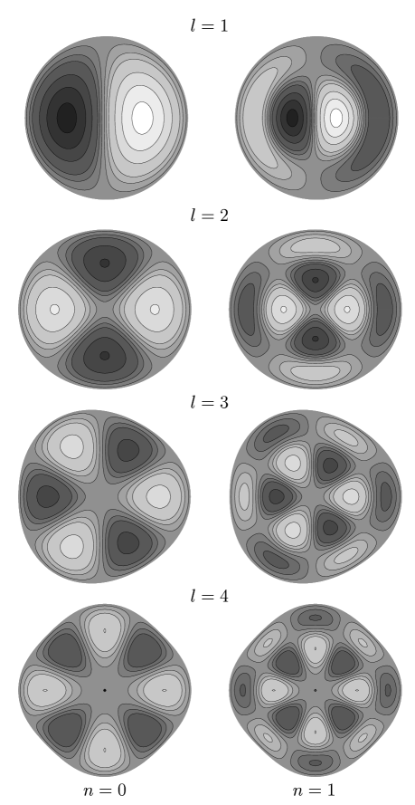
Figure 1: Density distributions (cut in the $(x,y)$–plane) of a droplet for the lowest collective modes with $n=0$ and 1 (left and right column, respectively) and $l=1$ to 4 (from top to bottom). Darker shades correspond to larger densities, lighter ones to smaller densities. The grey color in the center and at the border corresponds to the density of the undistorted sphere.

Deformations of the spherical droplet with homogenous density $\varrho$ and radius $R$ are conveniently described by a displacement field $\vec{s}(\vec{r},t)$. We introduce collective variables by the expansion coefficients $q_{\lambda}(t)$ of the displacement potential

$$w(\vec{r},t)=\sum_{\lambda}\,q_{\lambda}(t)\,\chi_{\lambda}(\vec{r})$$ (42)

and the corresponding irrotational displacement field

$$\vec{s}(\vec{r},t)=\vec{\nabla}\,w(\vec{r},t)=\sum_{\lambda}\,q_{\lambda}(t)\,\vec{\nabla}\chi_{\lambda}(\vec{r})\;.$$ (43)

Note that $q_{\lambda}$ has the dimension of (length)^7/2. The time derivative

$$\dot{\vec{s}}(\vec{r},t)=\sum_{\lambda}\,\dot{q}_{\lambda}(t)\,\vec{\nabla}\chi_{\lambda}(\vec{r})$$ (44)

determines the velocity field $\vec{v}$ at the position $\vec{r}+\vec{s}(\vec{r},t)$. This shift $\vec{s}(\vec{r},t)$ makes our expansion different from the one for the irrotational velocity field (1), which is commonly used (cf. b43 ). However, for $\vec{s}=0$ we have $\dot{\vec{s}}=\vec{v}(\vec{r})$, and hence all terms in (4), (5), (8) and (9), which are related to the collective kinetic energy, remain unchanged. Since for small amplitudes $B_{\lambda\lambda^{\prime}}=B_{\lambda\lambda^{\prime}}(\vec{q}_{0}=0)$, the kinetic energy part in (16) is not affected by the difference in the expansion. Of course, the stiffness coefficients are different due to the difference in the displacement fields. We have chosen the irrotational displacement field (43), because it conserves the center of mass exactly for all $l$-values including $l=1$ (cf. Appendix A.2), and furthermore allows to calculate mass and stiffness tensors analytically.

The density $\widetilde{\varrho}(\vec{r},t)$ varies according to the continuity equation

$$\frac{\partial\widetilde{\varrho}(\vec{r},t)}{\partial t}+\mbox{div}[\widetilde{\varrho}(\vec{r},t)\,\vec{v}(\vec{r},t)]=0\;,$$ (45)

which assures mass conservation. Figure 1 illustrates shapes and density profiles (calculated from eq. (80) of Appendix A.3) for the lowest collective modes with $n=0,1$ and $l=1,2,3,4$. Since we want to describe the fragmentation into at least two large fragments, we restrict the expansion (42) to $l\geq 2$. Instabilities with $l=0$ and $l=1$ are expected to lead essentially to a single heavy fragment with additional light particles ($n,p,d,\alpha$…), and hence can not be easily distinguished from evaporation events.

As discussed in Appendix A.3, the homogeneous sphere $(\vec{q}=0)$ is an equilibrium point in the space of the collective variables $q_{\lambda}$ for $l>0$, and hence (16) with $g_{\lambda}\rightarrow q_{\lambda}$ describes its harmonic modes.

3.1.2 Mass tensor

The mass (inertial) tensor $B_{\lambda\lambda^{\prime}}$ is calculated from the collective kinetic energy tensor. Every mass element $m_{N}\varrho\,\mathrm{d}^{3}r$ of the unperturbed droplet contributes $\frac{1}{2}m_{N}\varrho\,\mathrm{d}^{3}r[\dot{\vec{s}}(\vec{r},t)]^{2}$ to the kinetic energy (cf. (76)), where $m_{N}$ denotes the nucleon mass and $\varrho$ the constant value of the density inside the unperturbed sphere of radius $R$. Inserting the expansion (44) for $\dot{\vec{s}}(\vec{r},t)$ we obtain for the inertial tensor

$$B_{\lambda\lambda^{\prime}} = m_{N}\,\varrho\int_{r\leq R}\mathrm{d}^{3}r\,(\vec{\nabla}\chi_{\lambda})\cdot(\vec{\nabla}\chi_{\lambda^{\prime}})$$ (46)

$$= \delta_{\lambda\lambda^{\prime}}\,m_{N}\,\varrho\,\kappa_{nl}^{2}$$

according to the definition (9), where the final expression is diagonal and results from integrating by parts and using (38) and (40).

3.1.3 Stiffness tensor

According to the different energy contributions (intrinsic kinetic energy, local and nonlocal nuclear interaction, Coulomb and surface energies, cf. sect. 2.4), the adiabatic stiffness tensor

$$\overline{C}_{\lambda\lambda^{\prime}}=\overline{C}_{\lambda\lambda^{\prime}}^{(\tau)}+C_{\lambda\lambda^{\prime}}^{(V)}+C_{\lambda\lambda^{\prime}}^{(W)}+C_{\lambda\lambda^{\prime}}^{(C)}+C_{\lambda\lambda^{\prime}}^{(S)}$$ (47)

is the sum of five terms. The derivation of explicit formulae for the individual terms is straightforward. We refer to Appendix C for details.

The intrinsic kinetic energy term $\overline{C}_{\lambda\lambda^{\prime}}^{(\tau)}$ is calculated in the adiabatic limit, which is defined by leaving the occupation of the lowest single-particle levels unchanged. The final expression is

$$\overline{C}_{\lambda\lambda^{\prime}}^{(\tau)} = \sum_{i=n,p}\,2\epsilon_{\tau}^{(i)}(\varrho,T)\left\{\left(\frac{5}{9}+\frac{5}{3}\mu^{(i)}\right)\kappa_{nl}^{4}\,\delta_{\lambda\lambda^{\prime}}\right.$$ (48)

$$- \left.\left(\frac{4}{3}+2\mu^{(i)}\right)\frac{\kappa_{nl}\kappa_{n^{\prime}l}}{R^{2}}\,\delta_{ll^{\prime}}\delta_{mm^{\prime}}\right\}$$

with

$$\mu^{(i)}=\varrho\,m_{i}^{*}(\varrho)\frac{\mathrm{d}}{\mathrm{d}\varrho}\frac{1}{m_{i}^{*}(\varrho)}\;.$$ (49)

The kinetic energy density $\epsilon_{\tau}^{(i)}(\varrho,T)$ is defined by (27) and may be approximated by

$$\epsilon_{\tau}^{(i)}(\varrho,T)\approx\epsilon_{\tau}^{(i)}(\varrho,0)\,(1+\alpha T^{2})$$ (50)

with

$$\epsilon_{\tau}^{(i)}(\varrho,0)=\frac{3}{20}(3\pi^{2})^{2/3}\,\frac{\hbar^{2}\,\varrho_{i}^{5/3}}{m_{i}^{*}(\varrho)}\;,$$ (51)

$$\alpha=\frac{5}{3}\left(\frac{1}{9\pi}\right)^{2/3}\left(\frac{m_{i}^{*}(\varrho)}{\hbar^{2}}\right)^{2}\varrho_{i}^{-4/3}$$ (52)

for not too large temperatures $(T\ll\epsilon_{F}^{(i)})$, cf. b40* . The results, reported in sect. 4 have been obtained by using the exact expression (27). Since $(\kappa_{nl}R)^{2}\gg 1$, the first (diagonal) term is the largest contribution in (48).

The contribution from the nuclear-interaction density $\epsilon_{V}$ is obtained as

$$C_{\lambda\lambda^{\prime}}^{(V)} = {\varrho}^{2}\frac{\mathrm{d}^{2}\epsilon_{V}}{\mathrm{d}\varrho^{2}}\,\kappa_{nl}^{4}\,\delta_{\lambda\lambda^{\prime}}$$

$$- \left\{\varrho\frac{\mathrm{d}\epsilon_{V}}{\mathrm{d}\varrho}-\epsilon_{V}(\varrho)\right\}\frac{4\kappa_{nl}\kappa_{n^{\prime}l}}{R^{2}}\,\delta_{ll^{\prime}}\delta_{mm^{\prime}}\,.$$

The contributions from the Weizsäcker and Coulomb terms of the energy density are diagonal and read

$$C_{\lambda\lambda^{\prime}}^{(W)}=\frac{\mathrm{d}^{2}\epsilon_{W}}{\mathrm{d}(\nabla\varrho)^{2}}\,{\varrho}^{2}\,\kappa_{nl}^{6}\,\delta_{\lambda\lambda^{\prime}}\;,$$ (54)

$$C_{\lambda\lambda^{\prime}}^{(C)}=\frac{8\pi}{3}\,e_{0}^{2}\left(\frac{Z}{A}\varrho\right)^{2}\kappa_{nl}^{2}\,\delta_{\lambda\lambda^{\prime}}\;,$$ (55)

where $e_{0}$, $Z$ and $A$ denote the elementary charge and the charge and mass numbers of the nucleus, respectively.

For the surface energy contribution to the stiffness tensor we find

$$C_{\lambda\lambda^{\prime}}^{(S)}=4\epsilon_{S}(\varrho)\left\{9+\frac{1}{2}\,l(l+1)\right\}\,\frac{\kappa_{nl}\kappa_{n^{\prime}l}}{R^{3}}\,\delta_{ll^{\prime}}\delta_{mm^{\prime}}\;\;.$$ (56)

The stiffness tensor, as given by expressions (48),(49) and (3.1.3) to (56), is diagonal in $l$ and $m$ and not depending on $m$. The only couplings left are those corresponding to different $n$ values for the same multipolarity and are due to $\overline{C}_{\lambda\lambda^{\prime}}^{(\tau)},C_{\lambda\lambda^{\prime}}^{(V)}$ and $C_{\lambda\lambda^{\prime}}^{(S)}$.

Figure 2: Borders of compressional adiabatic spinodal instabilities in the $(\varrho,T)$-plane for infinite symmetric nuclear matter ($A$=$\infty$, heavy solid line), gold-like ($A$=197, $Z$=79, $N$=118, dashed line) and tin-like ($A$=100, $Z$=$N$=50, dotted line) nuclear droplets for a soft EOS (SkM^∗). Here, $\varrho_{0}=0.16$ fm^-3 is the normal nuclear matter density. Note that finite nuclei have central densities around $0.85\varrho_{0}$. The thin dashed lines indicate the expansion trajectories in the $(\varrho,T)$-plane at constant entropy $T\propto\varrho^{2/3}/m^{*}(\varrho)$ for infinite nuclear matter.

3.1.4 Infinite nuclear matter

The relation to thermodynamic properties of infinite nuclear matter is obtained by discarding Coulomb interactions and by taking the limit $R\to\infty$. Then $C^{(C)}$ and $C^{(S)}$ are negligible and $\kappa_{nl}\rightarrow\kappa$ is no longer restricted by (38) to discrete values. For any finite $\kappa$ we have $\kappa R\rightarrow\infty$, and hence

$$\overline{C}_{\lambda\lambda^{\prime}}=(c_{1}+c_{2}\,\kappa^{2})\kappa^{4}\,\delta_{\lambda\lambda^{\prime}}$$ (57)

with

$$c_{1}=\varrho\left(\frac{\mathrm{d}^{2}\overline{\epsilon}}{\mathrm{d}\varrho^{2}}\right),\quad\quad c_{2}=\varrho^{2}\left(\frac{\mathrm{d}^{2}\epsilon_{W}}{\mathrm{d}(\nabla\varrho)^{2}}\right),$$ (58)

$\overline{\epsilon}$ denoting the sum of the adiabatic kinetic and interaction energies. The eigenvalues are given by the dispersion relation

$$\omega^{2}=\overline{C}_{\lambda\lambda^{\prime}}/B_{\lambda\lambda}=\kappa^{2}(c_{1}+c_{2}\,\kappa^{2})/(m_{N}\varrho)\;,$$ (59)

a well-known result in infinite matter (cf. b44 ). In the adiabatic spinodal regime, i.e. in the $(\varrho,T)$-plane, where $c_{1}=\varrho(\mathrm{d}^{2}\epsilon/\mathrm{d}\varrho^{2})<0$, unstable modes with $\omega^{2}<0$ exist according to (59) for finite values of $\kappa$ up to a critical value $\kappa_{\mathrm{crit}}=\sqrt{-c_{1}/c_{2}}$. The border of the spinodal regime is determined by $\kappa_{\mathrm{crit}}=0$, i.e. $c_{1}=0$. At this point we immediately understand the large reduction of the spinodal region for finite systems (cf. fig. 2) by the finite values for the smallest $\kappa_{nl}$ determined by (38).

3.2 Pure surface modes

Pure surface modes, without any change of density inside, cannot be described by the expansion (43) for the displacement field $\vec{s}$. Instead, one has to use an expansion for the velocity field $\vec{v}$ satisfying $\vec{\nabla}\cdot\vec{v}=0$, such that the continuity equation (45) yields $\partial\widetilde{\varrho}/\partial t=0$ if $\widetilde{\varrho}=\varrho=const$ inside, initially. This problem is well studied and we essentially quote the results from b43 .

Figure 3: Contributions from the different terms (cf. eq. (47)) to the diagonal element of $B^{-1}C$ with $l=2$, $n=0$ for a hot ($T=4$ MeV) Au-like droplet ($Z,A=79,197)$ described by a soft EOS (SkM^∗). Also shown is the lowest eigenvalue $\omega^{2}$, which differs from $\overline{C}/B$ due to couplings with modes $n>0$.

Figure 4: The same as in fig. 3, but for a stiff EOS (SIII).

3.2.1 Collective variables

It is convenient to introduce real collective variables $Q_{lm}$, which describe the surface $r(\Omega)$ of the deformed droplet by the expansion

$$r(\Omega,t)=R\left(1+\sum_{lm}Q_{lm}{\cal Y}^{m}_{l}(\Omega)\right)\;,$$ (60)

where we use the real spherical harmonics (37) instead of the complex $Y^{m}_{l}(\Omega)$. The corresponding velocity field, which satisfies $\vec{\nabla}\cdot\vec{v}=0$, is defined by $v_{r}=\dot{r}$ at the undeformed surface, and hence by the irrotational field

$$\vec{v}(\vec{r},t)=\sum_{lm}\frac{\dot{Q}_{lm}}{l\,R^{l-2}}\vec{\nabla}(r^{l}{\cal Y}^{m}_{l})\;.$$ (61)

3.2.2 Mass tensor

The collective mass tensor is obtained from (46) by a partial integration, using $\Delta(r^{l}{\cal Y}^{m}_{l})=0$ and the Gauss integral formula. This yields the expression

$$B_{lm,l^{\prime}m^{\prime}}=\delta_{ll^{\prime}}\delta_{mm^{\prime}}\,m_{N}\varrho\frac{R^{5}}{l}\;,$$ (62)

where the $\vec{Q}$-dependence is neglected (harmonic or small-amplitude approximation).

3.2.3 Stiffness tensor

Since the density remains constant during the surface deformations, only the surface and Coulomb energies contribute to the stiffness tensor, i.e.

$$C_{lm,l^{\prime}m^{\prime}}=C_{lm,l^{\prime}m^{\prime}}^{(S)}+C_{lm,l^{\prime}m^{\prime}}^{(C)}\;.$$ (63)

In applying the expressions of b43 we note that

$$\alpha_{lm}=\frac{1}{\sqrt{2}}(Q_{lm}+iQ_{l-m})\;,$$ (64)

and hence $\sum_{m}|\alpha_{lm}|^{2}+|\alpha_{l-m}|^{2}=\sum_{m}Q_{lm}^{2}+Q_{l-m}^{2}$. Thus, also the stiffness tensors have to be equal to those of b43 ,

$$C_{lm,l^{\prime}m^{\prime}}^{(S)}=\delta_{ll^{\prime}}\delta_{mm^{\prime}}\,\frac{(l-1)(l+2)}{4\pi}\,a_{s}A^{2/3}\;,$$ (65)

$$C_{lm,l^{\prime}m^{\prime}}^{(C)}=-\delta_{ll^{\prime}}\delta_{mm^{\prime}}\,\frac{3}{2\pi}\,\frac{l-1}{2l+1}\frac{e_{0}}{r_{0}}\,Z^{2}\,A^{-1/3}\;,$$ (66)

which are diagonal and independent of $m$ like the mass tensor.

4 Results on stability and instability

According to (33) the eigenmode frequencies are obtained by a numerical diagonalization of the matrix $B^{-1}C$. We present detailed results on stability and instability of bulk and surface modes as functions of $\varrho$ and $T$. The calculations have been performed with the Skyrme energy densities, SkM^∗ and SIII (cf. Table 1), implying soft and stiff equations of state (EOS), respectively. We present here mainly the results for the soft equation of state (SkM^∗), because it is favored e.g. by the study of monopole vibrations and supernova explosions.

Figure 5: Eigenvalues $\omega^{2}$ for different compressional modes of quadrupole oscillations $(l=2)$ as functions of density at temperature $T=3$ MeV. Results for a gold-like droplet described by a soft EOS (SkM^∗) are presented. The diagonal contributions are displayed as thin lines, while the heavy lines represent the results obtained by diagonalization.

Figure 6: Lowest eigenvalues $\omega^{2}$ for the multipoles $l=2,3,4,5$ as functions of density at temperature $T=3$ MeV. Results for a gold-like droplet are presented for the soft EOS. Note that the line for $l=2$ is the lowest eigenvalue $\omega^{2}$ shown as heavy line in fig. 5

4.1 Compressional (bulk) modes

The results on compressional modes are presented in figs. 2–7.

4.1.1 Finite-size effects

In fig. 2 we illustrate effects of finite size on the region of instability in the ($\varrho,T$)-plane, where $\varrho$ and $T$ denote the density and temperature of the homogeneous droplet. As discussed in sect. 3.1.4, the spinodal line for infinite nuclear matter is determined by $\mathrm{d}^{2}\overline{\epsilon}/\mathrm{d}\varrho^{2}=0$ and is shown by the heavy solid line. For finite nuclei the spinodal regime is considerably reduced as shown for the gold- and tin-like nuclear droplets with $Z,A=79,197$ and $50,100$, respectively. The spinodal line is determined by the $l=2$ modes, as will be discussed below.

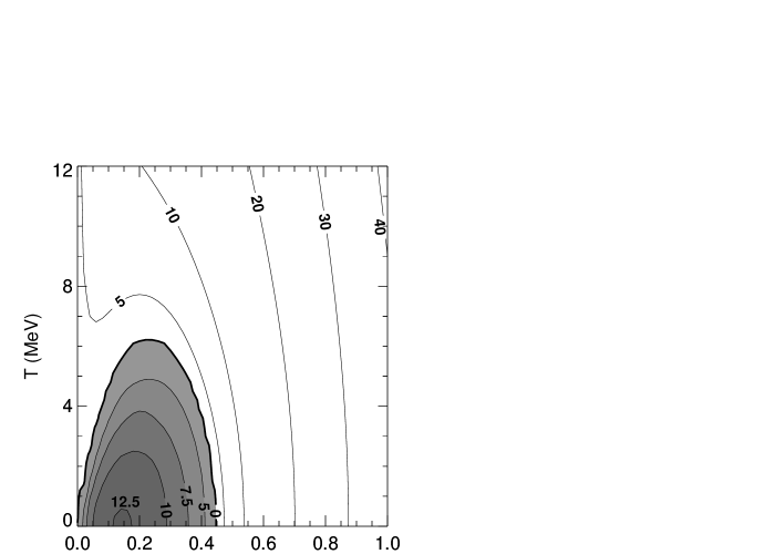
Figure 7: Lowest vibrational energies $\hbar\omega$ (in MeV) in the stable (white) region and largest growth rate $\gamma=\hbar\,\sqrt{-\omega^{2}}$ (in MeV) in the unstable (shaded) region as functions of $\varrho$ and $T$ for a gold-like droplet described by a soft EOS (SkM^∗). All modes with $l=2,3,4,5$ and $n=0,1,2,3,4,5$ are taken into account. To obtain the growth time $\hbar/\gamma$ in fm/c one has to divide 197 by the $\gamma$ value given in the shaded area.

4.1.2 Main contributions

Figure 3 shows quantitatively the importance of different contributions to the lowest eigenvalue $\omega^{2}$ as function of the density for $l=2$ at a temperature of 4 MeV. The eigenvalues are determined essentially only by the terms $C^{(\tau)},C^{(V)}$ and $C^{(W)}$, which are due to the intrinsic kinetic energy and the nuclear interaction parts $\epsilon_{V}$ and $\epsilon_{W}$. The contributions from Coulomb interactions and surface energy are negligible, which is well known for compression modes b43 . Figure 3 also reveals that the additional Weizsäcker contribution is the main reason for the reduction of the spinodal region in the finite systems, cf. the discussion at the end of sect. 3.1.4. Since $\kappa_{nl}=0$ on the spinodal line of an infinite system $(R\rightarrow\infty)$, the Weizsäcker term does not contribute. The difference between the spinodal lines for $A=100$ and $A=197$ is only marginal, because $R\propto A^{1/3}$ and $\kappa_{nl}\propto A^{-1/3}$.

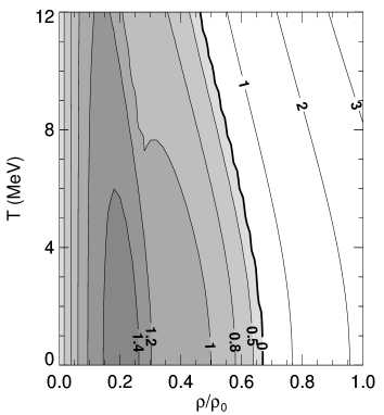
Figure 8: Contour plot of stability and instability for the surface modes of a gold-like droplet in the $(\varrho,T)$-plane. Conventions of presentation are the same as in fig. 7.

Figure 4 illustrates how the contributions to $\omega^{2}$ change for the stiff EOS. The results are similar to those for the soft EOS, but with larger instability inside the spinodal region and larger stability outside.

4.1.3 Dependence on $n$ and $l$

With decreasing densities and temperatures more and more modes with $n>0$ become unstable for the same multipolarity $l$. This feature is illustrated in fig. 5, where the eigenvalues $\omega^{2}$ of the lowest modes for a gold-like system are displayed as functions of $\varrho$ at $T=3$ MeV. Effects of coupling between different $n$-modes are clearly seen near the crossings of the diagonal contributions. Such a behavior is typical for all multipole modes as well as for the soft and stiff EOS.

Figure 6 illustrates the lowest eigenvalues $\omega^{2}$ for different multipolarities $(l=2,3,4,5)$. With decreasing density below $0.3\varrho_{0}$ all eigenvalues for the different $l$-values become degenerate. This means that all multipole distortions have the same growth rate. Note that also the eigenvalues for different $n$-values become degenerate in this range of densities (cf. b26 ; b25 ). As is discussed in sect. 5.2, such a feature can be responsible for a power law in the fragment-mass distribution of multifragmentation.

4.1.4 Dependence on $\varrho$ and $T$

Figure 7 shows the lowest eigenvalues $\omega^{2}$ as functions of $\varrho$ and $T$ for a gold-like droplet described by a soft EOS (SkM^∗). For convenience the numbers on the contour lines are not the $\omega^{2}$-values but the vibration energies in the stable region and the growth rates in the unstable region. The stable vibration $\hbar\omega=28$ MeV of gold at $T=0$ is considerably larger than the quadrupole energy (20.6 MeV) given in b43 , the difference being due to the additional Weizsäcker term in our calculations. The spinodal line for $A=197$ of fig. 2 is identical with the 0-line in fig. 7. We note in passing that the inclusion of $l=1$ and $l=0$ modes gives only a marginal increase of the region of instability.

4.2 Surface modes

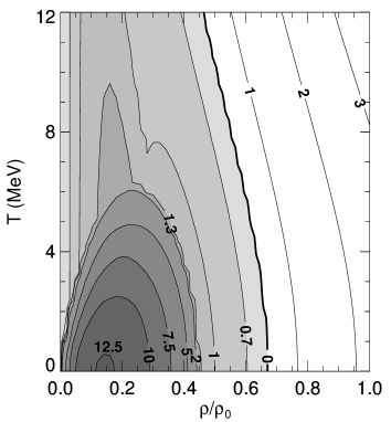
Figure 9: Combined bulk and surface instabilities (soft EOS) for a gold-like droplet. Shown are the largest growth rates and the lowest vibrational energies. Conventions of presentation are the same as in fig. 7.

The results are summarized in fig. 8. In contradistinction to fig. 7 for the compression modes the borderline between stability and instability for the surface modes is located at considerably larger densities near the spinodal line of infinite nuclear matter (by accident probably) and extends to high temperatures. This behavior is due to the softening of the surface tension with decreasing density and the weak temperature dependence. Thus, there is a wide region for large densities and temperatures, where the system becomes unstable with respect to surface deformations while being stable for compressional modes. However, the magnitudes of growth rates and vibrational energies of the surface modes are smaller by about half an order of magnitude as compared to the values for the compression modes. Note that the quadrupole mode is by far most unstable as seen from the $l$-dependence of the stiffness tensors (65) and (66).

Figure 10: The same as in fig. 9, but for tin-like droplet.

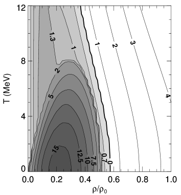
Figure 11: The same as in fig. 9 but for a stiff EOS .

4.3 Combined bulk and surface modes

A combined contour plot of compression and surface instabilities is presented in fig. 9. Compression instabilities are dominant at small densities and temperatures, while for large temperatures and densities only the surface modes are unstable.

4.3.1 Dependence on size

Figure 10 illustrates the regions of stability and instability for a tin-like droplet. As already shown in fig. 2, the compression instabilities of finite nuclear droplets depend only weakly on their masses $A$. The depth of the compression instability hole (dark regions) remains almost the same for the gold- and tin-like droplets. However, due to the sensitive balance between Coulomb and surface energies, the surface instabilities are pushed towards smaller densities for the lighter system.

4.3.2 Dependence on EOS

For the same mass of the droplet the regions of instability depend on the EOS. Figure 11 displays the combined instabilities for the gold-like droplet and a stiff EOS. Comparing the plot with fig. 9 we realize that the compression instabilities extend to higher temperatures for the stiff EOS (up to 8 MeV, as compared to about 6 MeV for the soft EOS) and to somewhat larger densities. In addition, the depth of the compression instability hole is substantially larger for the stiff EOS. The values for the growth rates reported for $\varrho=0.37\varrho_{0}$, $T=0$ in b26 , $\varrho=0.3\varrho_{0}$, $T=3$ MeV in b27 and $\varrho=0.3\varrho_{0}$, $T=6$ MeV in b24 are consistent with the values in the contour plot of fig. 11.

5 Instabilities and multifragmentation

As compared to infinite nuclear matter the spinodal region of the bulk (compression) instabilities is significantly reduced in finite systems (cf. fig. 2). However, finite systems exhibit additional modes due to the surface. Surface instabilities arise in finite systems already below $\varrho/\varrho_{0}\approx 0.6$ and extend to high excitation energies of the system (cf. fig. 8) for $A\approx 200$. Therefore in addition to bulk instabilities, surface instabilities become important in multifragmentation reactions. A heated nuclear droplet expands essentially at constant entropy (cf. fig. 2, b45 ), and hence experiences, with increasing initial excitation energy, first surface instabilities and then bulk instabilities. When reaching the spinodal regime the temperatures are of the order of about 5 MeV. In the following we discuss possible effects from surface and bulk instabilities, which become important during the expansion of the hot pieces of nuclear matter formed initially in fragmentation reactions.

5.1 Effects from surface instabilities

Hot spherical nuclei are formed initially most likely in high-energy target and projectile fragmentation reactions, as well as in bombardments of heavy nuclei with light particles $(p,d,\alpha,\ldots)$. If such hot nuclei are formed with excitation energies in the range 2.5 MeV $\lesssim E^{*}/A\lesssim 5$ MeV (6 MeV$\lesssim T\lesssim 9$ MeV) we expect b45 expansion into spinodal region of surface instabilities. Since quadrupole deformations $(l=2)$ are by far the most unstable surface modes (cf. eqs. (65),(66)), partition into two fragments of almost equal size ($A_{f}\approx A/2$) is most likely. This type of fragmentation differs qualitatively from the normal fission mechanism, because it happens at low densities, where no barrier is present any more.

In central collisions of (almost) equal nuclei at bombarding energies $\gtrsim$ 100 MeV/u one expects large dynamical distortions of the nuclear matter b46 . Because of the large times which are necessary to restore spherical symmetry (according to fig. 8 these times are of the order of (100-200) fm/c), the deformed hot matter will expand (typical time 30 fm/c) into the instability regime and fragment by pure surface instability plus dynamical collective motion or by additional bulk instabilities.

5.2 Effects from bulk (compressional) instabilities

For hot spherical nuclei formed at excitation energies $E^{*}/A$ $\gtrsim 5$ MeV ($T\gtrsim 9$ MeV) we expect b45 expansion into the spinodal regime of bulk instabilities. Near the spinodal line (of bulk instabilities, cf. fig. 6) quadrupole instabilities are most likely to develop. However, as one proceeds in reaching smaller densities modes with larger $l$-values and also larger $n$-values (cf. fig. 5 and 6) become unstable, reaching equal growth times for $\varrho/\varrho_{0}\lesssim 0.25$.

This feature leads naturally to a power law in the fragment mass distribution. In an instability mode, which leads to $m$ fragments, one produces fragments with mass $A_{f}=A/m$ with probability

$$P_{m}(A/m)\propto m^{2}\;,$$ (67)

where the second factor $m$ is due to the degeneracy of this mode. Since $m=A/A_{f}$ we find

$$P(A_{f})\propto A_{f}^{-2}$$ (68)

for the fragment mass distribution. Of course, such a behavior can only be expected for $m>2$, and hence $A_{f}$ well below $A/2$. We stress that the power-law behavior (68) is due only to the degeneracy of growth times for different modes $n,l$, and not related to the critical point.

5.3 General aspects of fragment-mass distributions

According to expansion and instabilities of spherical droplets we expect the following qualitative features for the fragment-mass distribution with two or more heavy fragments.

• For low energies only fission-like fragmentation should occur which give rise to a bump around $A_{f}\lesssim A/2$ and emitted light particles with an exponentially decreasing mass distribution.

• For energies 5 MeV $<E^{*}/A<$ 8 MeV, which lead to expansion just into the spinodal region of bulk instabilities, the fragmentation is governed by low $l$-values ($l=1,2,3$). According to fig. 1 large regions of low densities are produced in the development of these low-$l$ instabilities. The subsequent fragmentation of these will lead to a power-law behavior for light fragments in addition to the heavy fragments and their evaporated light particles.

• For energies 8 MeV $<E^{*}/A<$ 12 MeV, which lead to expansion well into the region of bulk instabilities for densities $\varrho/\varrho_{0}<0.3$, a pure power law with $\sigma=2.0$ is expected for the fragment mass distribution.

These properties of fragment-mass distributions are well established by experiments, cf. b38 . The observed larger values of $\sigma$ for $E^{*}/A>$ 12 MeV indicate that the freeze-out of fragments is probably faster than allowed by growth rates of instabilities, e.g. by a coalescence mechanism.

5.4 Experimental prospects

It is not clear how those components of the multifragmentation process can be identified, which are due to spinodal decomposition. A possible strategy is to analyze the data event by event and to look for characteristic modes as function of initial excitation energy b27 ; b47 . An indication for spinodal decomposition has been reported recently b28 .

Of course, one should look particularly into fragmentation reactions, which are favorable for spinodal decomposition occurring in large dilute spherical droplets. As mentioned earlier in sect. 5.1, central heavy-ion collisions exhibit violent collective deformations, and hence will have complicated dynamics, which may mask the spinodal decomposition phenomena.

In projectile and target fragmentation at high bombarding energies the excitation by abrasion yields excited spectators without large dynamical distortion. Thus we can expect that a large fraction in the multifragmentation process is due to spinodal decomposition after expansion. However, induced by the abrasion process, certain parts of projectile and target will be emitted initially before expansion. This component, which may contribute of order 10% to the fragment yield, is characterized by considerably larger fragment kinetic energies. During the fast expansion the number of emitted particles is small b45 , such that we expect only two relevant components, one from the initial excitation process and another one from the break-up after expansion.

A recent analysis b48 of the decay of target spectators in ¹⁹⁷Au+¹⁹⁷Au collisions at 1 GeV/u has indicated that the fragments are already produced at the initial matter densities. However, we would like to interpret the observed fragment kinetic energy spectra as evidence for a high- and low-energy component, which correspond to initial excitation process and the break-up after expansion, respectively. Such a picture is supported by the decrease of the He-Li temperatures from (10–12) MeV in the high-energy tails to about 5 MeV in the low-energy part of the fragment kinetic-energy distribution. The evolutionary character of the multifragmentation process from initial excitation via expansion to the final break-up is supported by the analysis of central ¹²⁹Xe+^natCu at 30 MeV/u b54* and light-ion induced fragmentation reactions b52* .

Acknowledgements

We gratefully acknowledge fruitful discussions with our experimental colleagues U. Lynen, W. Trautmann and C. Schwarz.

Appendix

Appendix A The displacement transformation

Displacement transformations have been frequently used in the description of small-amplitude collective nuclear motion b49 ; b50 ; b51 ; b52 . With the introduction of the displacement for wave functions in a differential form it was possible to extend such descriptions to large-amplitude dissipative collective motion, cf. sect. 2.1. Within this approach a scaling condition (2) for the stationary part of the diabatic single-particle wave functions, written here as

$$\frac{\partial}{\partial t}\widetilde{\phi}(\vec{r},t)=-\frac{1}{2}[\vec{v}(\vec{r},t)\cdot\vec{\nabla}+\vec{\nabla}\cdot\vec{v}(\vec{r},t)]\,\widetilde{\phi}(\vec{r},t)\;,$$ (69)

assures that all dynamical couplings linear in the velocities disappear in the Schrödinger equation for the time-dependent wave function. Considering this equation (69) at the time dependent point $\vec{r^{\prime}}=\vec{r}+\vec{s}(\vec{r},t)$ we find with $\dot{\vec{s}}(\vec{r})=\vec{v}(\vec{r}+\vec{s}(\vec{r}))$ for the total derivative

$$\frac{\mathrm{d}}{\mathrm{d}t}\widetilde{\phi}(\vec{r}+\vec{s}(\vec{r},t),t)=\widetilde{\phi}(\vec{r}+\vec{s}(\vec{r},t),t)\,(-\frac{1}{2}\vec{\nabla}^{\prime}\cdot\dot{\vec{s}}(\vec{r}))\;,$$ (70)

where $\vec{\nabla}^{\prime}$ denotes the gradient vector taken at the position $\vec{r^{\prime}}$. After integration from $t=0,s=0$ to $t,\vec{s}(t)$

$$\widetilde{\phi}(\vec{r}+\vec{s}(\vec{r},t),t)=\phi(\vec{r})\exp\{-\frac{1}{2}\vec{\nabla}^{\prime}\cdot\vec{s}(\vec{r},t)\}\;,$$ (71)

i.e. the value of the transformed wave function at the point $\vec{r^{\prime}}=\vec{r}+\vec{s}(\vec{r},t)$ is given by the original wave function $\phi(\vec{r})$ at the point $\vec{r}$ normalized to ensure the unitarity of the transformation as implied by the integrated eq. (69),

$$\widetilde{\phi}(\vec{r^{\prime}},t)=\exp\{-\frac{1}{2}[\vec{s}(\vec{r},t)\cdot\vec{\nabla}^{\prime}+\vec{\nabla}^{\prime}\cdot\vec{s}(\vec{r},t)]\}\,\widetilde{\phi}(\vec{r^{\prime}},0)\;.$$ (72)

Recently,  similar unitary displacement transformations have been successfully implemented in the treatment of two-body correlations caused by realistic two-body interactions b53 .

A.1 Continuity equation, particle conservation

Defining the total single-particle density by the sum over all occupied states, we find as a consequence of (71)

$$\widetilde{\varrho}(\vec{r}+\vec{s}(\vec{r},t),t)=\varrho(\vec{r})\,\mbox{e}^{-(\vec{\nabla}^{\prime}\cdot\vec{s}(\vec{r},t))}\,,$$ (73)

where $\varrho(\vec{r})$ is the density of the undistorted sphere. In differential form this equation becomes (cf. (70))

$$\frac{\mathrm{d}\widetilde{\varrho}(\vec{r^{\prime}},t)}{\mathrm{d}t}=-\widetilde{\varrho}(\vec{r^{\prime}},t)(\vec{\nabla}^{\prime}\cdot\dot{\vec{s}}(\vec{r},t))$$ (74)

and, since $\dot{\vec{s}}(\vec{r},t)=\vec{v}(\vec{r}+\vec{s}(\vec{r}),t)$, we find the continuity equation

$$\frac{\mathrm{d}\widetilde{\varrho}(\vec{r^{\prime}},t)}{\mathrm{d}t}+\widetilde{\varrho}(\vec{r^{\prime}},t)\,(\vec{\nabla}\cdot\vec{v})_{\vec{r^{\prime}}}=0\;,$$ (75)

which also results form (45) by considering the substantial change of density $\mathrm{d}\widetilde{\varrho}(\vec{r^{\prime}})/\mathrm{d}t$ along the displacement path, i.e. in the comoving frame.

Particle conservation implies

$$\mathrm{d}^{3}r^{\prime}\,\widetilde{\varrho}(\vec{r^{\prime}})=\mathrm{d}^{3}r\,\varrho(\vec{r})\;,$$ (76)

which means, that the number of particles in a volume element is conserved when followed in the distortion process.

A.2 Conservation of the center of mass

The time derivative of the center of mass

$$\frac{\mathrm{d}}{\mathrm{d}t}\langle\vec{r}\rangle=\frac{1}{A}\int\mathrm{d}^{3}r^{\prime}\,\widetilde{\varrho}(\vec{r^{\prime}})\,\vec{v}(\vec{r^{\prime}},t)$$ (77)

should vanish. This integral is rewritten as

$$\frac{\mathrm{d}}{\mathrm{d}t}\langle\vec{r}\rangle=\frac{1}{A}\int\mathrm{d}^{3}r\,\varrho(\vec{r})\,\dot{\vec{s}}(\vec{r},t)\;,$$ (78)

by using (76) and $\vec{v}(\vec{r^{\prime}},t)=\dot{\vec{s}}(\vec{r},t)$ with $A$ and $\varrho(\vec{r})$ denoting the mass number and the unperturbed density distribution, respectively. This equation is understood by noting that the mass element positioned at $\vec{r}$ for $\vec{s}=0$ contributes for $\vec{s}\neq 0$ at the point  $\vec{r}+\vec{s}(\vec{r},t)$ to the center of mass. Since $\vec{s}$ is given by (43) we find by partial integration of (78) that

$$\frac{\mathrm{d}}{\mathrm{d}t}\langle\vec{r}\rangle\propto\sum_{\lambda}\dot{q}_{\lambda}\,\chi_{\lambda}(R,\Omega)=0\,,$$ (79)

i.e. for every multipole distortion (even for $l=1$) the center of mass is conserved exactly.

A.3 Second-order expansion of density

Expanding (73) to second order in $\vec{s}$, we find

$$\widetilde{\varrho}(\vec{r}+\vec{s},t)=\varrho(\vec{r})\,[(1-\vec{\nabla}\cdot\vec{s}+\frac{1}{2}(\vec{\nabla}\cdot\vec{s})^{2}-(\vec{\nabla}^{\prime}-\vec{\nabla})\cdot\vec{s}]\;.$$ (80)

The last term can be rewritten in second order as

$$-(\vec{\nabla}^{\prime}-\vec{\nabla})\cdot\vec{s}=\frac{1}{2}\sum_{i,j}(\partial_{i}\partial_{j}\,w)^{2}\;,$$ (81)

where $\partial_{i}$ denotes the differentiation with respect to the $i$’th cartesian component of $\vec{r}$. From (40),(42) and (43) we obtain

$$-\vec{\nabla}\cdot\vec{s}=-\sum_{\lambda}\,q_{\lambda}\Delta\chi_{\lambda}=\sum_{\lambda}\,q_{\lambda}\,\kappa_{nl}^{2}\,\chi_{\lambda}\;.$$ (82)

The integral $\int_{r\leq R}\,\mathrm{d}^{3}r\,\vec{\nabla}\cdot\vec{s}=0$, because the integral over the single spherical harmonic in $\chi_{\lambda}$ vanishes for $l>0$. This property causes the first-order derivative of the total energy of the spherical droplet to vanish, and hence the spherical droplet is an equilibrium point with respect to the displacement field.

For the derivatives of the density with respect to the collective coordinates $q_{\lambda}$ we obtain the relations

$$\left(\frac{\partial\widetilde{\varrho}}{\partial q_{\lambda}}\right)_{\vec{q}=0}=\varrho(\vec{r})\,\kappa_{nl}^{2}\,\chi_{\lambda}(\vec{r})$$ (83)

and

$$\left(\frac{\partial^{2}\widetilde{\varrho}}{\partial q_{\lambda}\partial q_{\lambda^{\prime}}}\right)_{\vec{q}=0} = \varrho(\vec{r})\,[\kappa_{nl}^{2}\kappa_{n^{\prime}l^{\prime}}^{2}\,\chi_{\lambda}(\vec{r})\chi_{\lambda^{\prime}}(\vec{r})$$

$$+\sum_{i,j}(\partial_{i}\partial_{j}\chi_{\lambda})(\partial_{i}\partial_{j}\chi_{\lambda^{\prime}})]\;,$$

which frequently appear in the evaluation of the stiffness tensor (cf. Appendix C).

Appendix B Surface tension

The surface interaction energy $E^{LD}_{S}$ of a sphere with radius $R$ is determined by the difference

$$E^{LD}_{S}=E_{V}+E_{W}-E^{LD}_{V}$$ (85)

of the local and nonlocal interaction energies $E_{V}+E_{W}$ for the diffusive sphere and the interaction energy $E^{LD}_{V}$ of the homogeneous sphere with the constant density $\varrho$ in the interior $(r<R)$.

Assuming a linear approximation

$$\widetilde{\varrho}(r,t)=\frac{1}{2}\varrho\left(1-\frac{r-R}{2a}\right)\quad\mbox{for}\quad|r-R|\leq 2a$$ (86)

to the Fermi function for describing the transition of the density from the inside to the outside ($a$ denoting the diffuseness parameter) we obtain for $R\gg a$ (leptodermous system)

$$E_{V}-E^{LD}_{V}=-4\pi R^{2}\,\frac{2}{3}e_{V}\varrho^{2}a\;,$$ (87)

$$E_{W}=4\pi R^{2}\,\frac{1}{4}e_{W}\frac{\varrho^{2}}{a}\;.$$ (88)

Here, the energy densities $\epsilon_{V}=e_{V}\varrho^{2}(r,t)$ and $\epsilon_{W}=e_{W}(\vec{\nabla}\varrho)^{2}$ have been used. Dividing by the surface $4\pi R^{2}$, we find the surface tension

$$\epsilon_{S}=\varrho^{2}\left(-\frac{2}{3}e_{V}a(T)+\frac{1}{4}\frac{e_{W}}{a(T)}\right)\;,$$ (89)

where $a(T)$ increases with increasing temperature. According to b54 $a(T)/a(0)-1\propto T^{2}$, and hence

$$\epsilon_{S}(\varrho,T)=\epsilon_{S}(\varrho_{\mathrm{eq}},0)\,\left(\frac{\varrho}{\varrho_{\mathrm{eq}}}\right)^{2}(1+\beta T^{2})\;.$$ (90)

Introducing the explicite form for $\epsilon_{S}(\varrho_{\mathrm{eq}},0)$ with the asymmetry dependence on neutron and proton numbers, we finally obtain eq. (32) with the values $\beta$ from b41 ; b42 .

Appendix C Evaluation of the stiffness tensor

The evaluation of the different contributions to the stiffness tensor (47) is simplified by considering the displacement of individual volume elements with the displacement field $\vec{s}(\vec{r})$. Then according to (76), the integrals over the distorted sphere can be replaced by integrals over the original volume elements. In this way only integrals over the original sphere of radius $R$ have to be evaluated.

C.1 Intrinsic kinetic energy contribution $C_{\lambda\lambda^{\prime}}^{(\tau)}$

In the local-density approximation the intrinsic kinetic energy for protons or neutrons is given by

$$E_{\mathrm{kin}}^{\mathrm{intr}}=\int_{r\leq R}\,\mathrm{d}^{3}r\frac{\hbar^{2}}{2m^{*}(\widetilde{\varrho})}\,\int\mathrm{d}^{3}k\,f(k)\widetilde{\vec{k}}^{2}\;,$$ (91)

where $f(k)$ denotes the (isotropic) momentum distribution within the unperturbed droplet normalized to $\varrho$. Due to the distortion, the local momentum $\vec{k}$ transforms to $\widetilde{\vec{k}}$. In the adiabatic limit the density dependence of $\langle\widetilde{\vec{k}}^{2}\rangle\propto\widetilde{\varrho}^{2/3}$ enters, and hence with the density (80) at the displaced volume element we obtain

$$\langle\widetilde{\vec{k}}^{2}\rangle=\langle\vec{k}^{2}\rangle\{1-\frac{2}{3}\vec{\nabla}\cdot\vec{s}+\frac{7}{18}(\vec{\nabla}\cdot\vec{s})^{2}+\frac{1}{3}\sum_{i,j}(\partial_{i}\partial_{j}\,w)^{2}\}$$ (92)

up to second order in the displacement field $\vec{s}$.

In the final evaluation of

$$C_{\lambda\lambda^{\prime}}^{(\tau)} = \left(\frac{\partial^{2}\,E_{\mathrm{kin}}^{\mathrm{intr}}}{\partial q_{\lambda}\partial q_{\lambda^{\prime}}}\right)_{\vec{q}=0}$$

$$= \varrho\int\mathrm{d}^{3}r\frac{\hbar^{2}}{2}\left\{\frac{\partial^{2}}{\partial q_{\lambda}\partial q_{\lambda^{\prime}}}\frac{\langle\widetilde{\vec{k}}^{2}\rangle}{m^{*}(\widetilde{\varrho})}\right\}_{\vec{q}=0}$$

we encounter integrals

$$\int\mathrm{d}^{3}r(\vec{\nabla}\cdot\vec{s})^{2}=\sum_{\lambda}\,q_{\lambda}^{2}\,\kappa_{nl}^{4}$$ (94)

and

$$\sum_{i,j}\,\int\mathrm{d}^{3}r\,(\partial_{i}\partial_{j}\chi_{\lambda})(\partial_{i}\partial_{j}\chi_{\lambda^{\prime}}) =$$ (95)

$$\int\mathrm{d}^{3}r\,\{\sum_{i,j}\partial_{i}[(\partial_{j}\chi_{\lambda})(\partial_{i}\partial_{j}\chi_{\lambda^{\prime}})] - (\partial_{j}\chi_{\lambda})\partial_{i}\partial_{i}(\partial_{j}\chi_{\lambda^{\prime}})\}\,.$$

Here, starting with (C.1), and in the following we imply that integration over $\vec{r}$ is limited to the unperturbed sphere $(r\leq R)$. In (95) the second term on the r.h.s. is evaluated using $\sum_{i}\partial_{i}\partial_{i}=\Delta$ and (40) twice (on the way one more integration by parts and transformation to a surface integral that vanishes as $\chi_{\lambda}(R)=0$), which leads to

$$\int\mathrm{d}^{3}r\,(\partial_{j}\chi_{\lambda})\partial_{i}\partial_{i}(\partial_{j}\chi_{\lambda^{\prime}})=\kappa_{nl}^{2}\kappa_{n^{\prime}l^{\prime}}^{2}\,\delta_{\lambda\lambda^{\prime}}\,.$$ (96)

The first term on the r.h.s. of (95) is transformed to the symmetric form

$$\sum_{i,j}\int\mathrm{d}^{3}r\,\partial_{i}[(\partial_{j}\chi_{\lambda})(\partial_{i}\partial_{j}\chi_{\lambda^{\prime}})] =$$ (97)

$$\frac{1}{2}\sum_{i,j}\int\mathrm{d}^{3}r\,\partial_{i}\partial_{i}(\partial_{j}\chi_{\lambda}\partial_{j}\chi_{\lambda^{\prime}}) = -\frac{4\kappa_{nl}\kappa_{n^{\prime}l^{\prime}}}{R^{2}}\,\delta_{ll^{\prime}}\delta_{mm^{\prime}}\,.$$

The latter result is obtained by transforming to a surface integral and utilizing the properties of derivatives of Bessel functions on the surface,

$$j^{\prime\prime}_{l}(\kappa_{nl}R)=-\frac{2}{\kappa_{nl}R}\,j^{\prime}_{l}(\kappa_{nl}R)\;,$$ (98)

which result from their differential equation taken at
$r=R$.

The final result given by eq. (48) is obtained by putting all terms together, including the linear density dependence of $(m^{*}(\widetilde{\varrho}))^{-1}$ and summing over protons and neutrons.

C.2 Interaction-energy contribution $C_{\lambda\lambda^{\prime}}^{(V)}$

This term is calculated from the expression

$$C_{\lambda\lambda^{\prime}}^{(V)}=\left\{\frac{\partial^{2}}{\partial q_{\lambda}\partial q_{\lambda^{\prime}}}\int\mathrm{d}^{3}r^{\prime}\,\epsilon_{V}(\widetilde{\varrho}(\vec{r}^{\prime}))\right\}_{\vec{q}=0}\;.$$ (99)

With the explicit introduction of the displacement field $\vec{s}(\vec{r})$ we can transform the integral over $\vec{r}^{\prime}$ to an integral over $\vec{r}=\vec{r}^{\prime}-\vec{s}(\vec{r},t)$ by replacing $\mathrm{d}^{3}r^{\prime}$ by $\mathrm{d}^{3}r\,\varrho(\vec{r})/\widetilde{\varrho}(\vec{r}^{\prime})$. We find

$$C_{\lambda\lambda^{\prime}}^{(V)} = 2\left(\frac{1}{2}\frac{\partial^{2}\epsilon_{V}(\varrho)}{\partial\varrho^{2}}-\frac{1}{\varrho}\frac{\partial\epsilon_{V}(\varrho)}{\partial\varrho}+\frac{\epsilon_{V}(\varrho)}{\varrho^{2}}\right)$$

$$\times\int\mathrm{d}^{3}r\,\left(\frac{\partial\widetilde{\varrho}}{\partial q_{\lambda}}\frac{\partial\widetilde{\varrho}}{\partial q_{\lambda}^{\prime}}\right)_{\vec{q}=0}$$

$$+\left(\frac{\partial\epsilon_{V}(\varrho)}{\partial\varrho}-\frac{\epsilon_{V}(\varrho)}{\varrho}\right)\int\mathrm{d}^{3}r\,\left(\frac{\partial^{2}\widetilde{\varrho}}{\partial q_{\lambda}\partial q_{\lambda}^{\prime}}\right)_{\vec{q}=0}\;,$$

where $\varrho(\vec{r})=\varrho$ for $r\leq R$ is used. Insertion of (83), (A.3) and (97) yields the result given by (3.1.3).

C.3 Weizsäcker-energy contribution $C_{\lambda\lambda^{\prime}}^{(W)}$

This term is calculated from the expression

$$C_{\lambda\lambda^{\prime}}^{(W)}=e_{W}\left\{\frac{\partial^{2}}{\partial q_{\lambda}\partial q_{\lambda^{\prime}}}\int\mathrm{d}^{3}r^{\prime}\,(\vec{\nabla}\widetilde{\varrho})^{2}_{\vec{r^{\prime}}=\vec{r}+\vec{s}}\right\}_{\vec{q}=0}\;,$$ (101)

where $\epsilon_{W}=e_{W}\,(\vec{\nabla}\varrho)^{2}$ has been used. Note that the surface energy is treated explicitly below, and hence is excluded here. The integral over $r^{\prime}$ is again replaced by an integral over $r$. However, since $\vec{\nabla}\widetilde{\varrho}={\cal O}(q_{\lambda})$ we only need in second order $\partial\widetilde{\varrho}/\partial q_{\lambda}$ given by (83) without an additional contribution from the change of integration variable. By partial integration and using (38), (40) and (41) we find the result (54).

C.4 Surface-energy contribution $C_{\lambda\lambda^{\prime}}^{(S)}$

This term is calculated from the expression

$$C_{\lambda\lambda^{\prime}}^{(S)}=\left\{\frac{\partial^{2}}{\partial q_{\lambda}\partial q_{\lambda^{\prime}}}\int\mathrm{d}\widetilde{f}\,\epsilon_{s}(\widetilde{\varrho})\right\}_{\vec{q}=0}\;,$$ (102)

where the integration runs over the deformed surface

$$r(\Omega)=R+s_{r}(R,\Omega)$$ (103)

with the radial displacement

$$s_{r}=\sum_{\lambda}\,q_{\lambda}\frac{\kappa_{nl}}{R}\sqrt{\frac{2}{R}}\,{\cal Y}_{l}^{m}(\Omega)\;,$$ (104)

while the other components of $\vec{s}$ vanish (for $r=R$). Introducing (cf. b43 )

$$\mathrm{d}\widetilde{f}=\mathrm{d}\Omega\,r^{2}(\Omega)\sqrt{1+(\vec{\nabla}s_{r})^{2}}$$ (105)

for the deformed surface element, we are left with an integration over $\Omega$. One should note that $\vec{\nabla}s_{r}$ contains only angular derivatives. Furthermore, since $\epsilon_{S}(\widetilde{\varrho})$ is quadratic in $\widetilde{\varrho}$, we have ($\vec{\nabla}\cdot\vec{s}=0$ on the surface) up to second order in $\vec{s}$

$$\epsilon_{S}(\widetilde{\varrho},R) = \epsilon_{S}(\varrho)\{1-2(\vec{\nabla}^{\prime}-\vec{\nabla})\cdot\vec{s}\}_{r=R}$$

$$= \epsilon_{S}(\varrho)\left\{1+2\left(\frac{\partial s_{r}}{\partial r}\right)^{2}\right\}_{r=R}\;.$$

Thus we find

$$C_{\lambda\lambda^{\prime}}^{(S)} =\epsilon_{S}(\varrho) \left\{\frac{\partial^{2}}{\partial q_{\lambda}\partial q_{\lambda^{\prime}}}\right.$$

$$\left.\int\mathrm{d}\Omega\{9s_{r}^{2}(R)+R^{2}(\vec{\nabla}s_{r}(R))^{2}\}\right\}_{\vec{q}=0}\;,$$

where $(\partial s_{r}/\partial r)_{r=R}=-(2/R)s_{r}(R,\Omega)$ has been used (cf. eqs. (43), (98), (104)). Insertion of $s_{r}$ according to (43) and partial integration of the second term yields the expression (56) for the surface part of the stiffness tensor.

C.5 Coulomb-energy contribution $C_{\lambda\lambda^{\prime}}^{(C)}$

This term is defined by

$$C_{\lambda\lambda^{\prime}}^{(C)}=\left\{\frac{\partial^{2}}{\partial q_{\lambda}\partial q_{\lambda^{\prime}}}\frac{1}{2}\int\mathrm{d}^{3}r^{\prime}_{1}\mathrm{d}^{3}r^{\prime}_{2}\frac{\widetilde{\varrho}_{p}(\vec{r}^{\prime}_{1})\widetilde{\varrho}_{p}(\vec{r}^{\prime}_{2})}{|\vec{r}^{\prime}_{1}-\vec{r}^{\prime}_{2}|}\right\}_{\vec{q}=0}\;,$$ (108)

where $\vec{r}^{\prime}_{1}=\vec{r}_{1}+\vec{s}(\vec{r}_{1})$, $\vec{r}^{\prime}_{2}=\vec{r}_{2}+\vec{s}(\vec{r}_{2})$ and $\widetilde{\varrho}_{p}=e_{0}(Z/A)\widetilde{\varrho}$ denotes the charge density of the distorted sphere. Replacing the integration variables by $\vec{r}_{1}$ and $\vec{r}_{2}$ and using particle conservation $\mathrm{d}^{3}r^{\prime}\widetilde{\varrho}(\vec{r^{\prime}})=\mathrm{d}^{3}r\varrho(\vec{r})$ in the displacement from $\vec{r}$ to $\vec{r^{\prime}}=\vec{r}+\vec{s}(\vec{r})$ we find

$$C_{\lambda\lambda^{\prime}}^{(C)} = \frac{1}{2}\left(\frac{Ze_{0}}{A}\varrho\right)^{2}$$

$$\times \left\{\frac{\partial^{2}}{\partial q_{\lambda}\partial q_{\lambda^{\prime}}}\int\frac{\mathrm{d}^{3}r_{1}\mathrm{d}^{3}r_{2}}{|\vec{r}_{1}+\vec{s}(\vec{r}_{1})-\vec{r}_{2}-\vec{s}(\vec{r}_{2})|}\right\}_{\vec{q}=0}\;,$$

where the integrals are over $r_{1},r_{2}\leq R$ (the unperturbed sphere). The terms of the integral, which are of second order in $\vec{s}$ or $q_{\lambda}$ are given by the sum of $I_{1}$ and $I_{2}$. $I_{1}$ is defined by

$$I_{1}=\int\mathrm{d}^{3}r_{1}\mathrm{d}^{3}r_{2}\,[\vec{s}(\vec{r}_{1})\cdot\vec{\nabla}_{1}][\vec{s}(\vec{r}_{2})\cdot\vec{\nabla}_{2}]\frac{1}{|\vec{r}_{1}-\vec{r}_{2}|}\;.$$ (110)

Inserting $\vec{s}(\vec{r}_{2})=\vec{\nabla}_{2}w(\vec{r}_{2})$, integrating by parts over $\vec{r}_{2}$ (noting $w(R)=0$) and using $\Delta|\vec{r}_{1}-\vec{r}_{2}|^{-1}=-4\pi\delta(\vec{r}_{1}-\vec{r}_{2})$, we find

$$I_{1}=4\pi\int\mathrm{d}^{3}r(\vec{\nabla}w)^{2}\;.$$ (111)

$I_{2}$ is related to $I_{1}$ by

$$I_{2} = \int\mathrm{d}^{3}r_{1}\,\vec{s}(\vec{r}_{1})\cdot[\vec{s}(\vec{r}_{1})\cdot\vec{\nabla}_{1}]\,\vec{\nabla}_{1}\int\frac{\mathrm{d}^{3}r_{2}}{|\vec{r}_{1}-\vec{r}_{2}|}$$ (112)

$$= -\frac{2\pi}{3}\,\int\mathrm{d}^{3}r\,\vec{s}(\vec{r})\cdot[\vec{s}(\vec{r})\cdot\vec{\nabla}]\vec{\nabla}r^{2}=-\frac{1}{3}\,I_{1}\;.$$

Finally, by partial integration, using (82) and taking derivatives with respect to $q_{\lambda},q_{\lambda^{\prime}}$ we find the result given by (55).

References

- (1) L.G. Moretto and G.J. Wozniak, Annu. Rev. Nucl. Part. Sci. 43, 379 (1993)
- (2) B. Tamain and D. Durand, in Proceedings of the International School Trends in Nuclear Physics, 100 years later, Les Houches, Session LXVI, ed. by H. Nifenecker, J.-P. Blaizot, G.F. Bertsch, W. Weise and F. David (North-Holland, Amsterdam, 1998) p. 295
- (3) Proc. Sixth Int. Conf. on Nucleus–Nucleus Collisions, Gatlinburg, 1997, ed. by M. Thoennessen, F.E. Bertrand, J.D. Garrett and C.K. Gelbke, Nucl. Phys. A 630, 1c (1998) ; cf. also forthcoming Proc. Seventh Int. Conf. on Nucleus–Nucleus Collisions, Strasbourg, 3-7 July 2000, to be published in Nucl. Phys. A, (1/2001)
- (4) Multifragmentation, Proc. Int. Worksh. XXVII on Gross Properties of Nuclei and Nuclear Excitations, Hirschegg, 17-23 Jan. 1999, ed. by H. Feldmeier, J. Knoll, W. Nörenberg and J. Wambach (GSI, Darmstadt, 1999) ISSN 0720-8715
- (5) J.E. Finn et al., Phys. Rev. Lett. 49, 1321 (1982)
- (6) R.J. Lenk and V.R. Pandharipande, Phys. Rev. C 34, 177 (1986); T.J. Schlagel and V.R. Pandharipande, Phys. Rev. C 36, 162 (1987)
- (7) G. Peilert, H. Stöcker and W. Greiner, Rep. Prog. Phys. 57, 533 (1994)
- (8) J. Aichelin, Phys. Rep. 202, 233 (1991) and refs. therein.
- (9) L. Vinet, C. Gregoire, P. Schuck, B. Rémaud and F. Sébille, Nucl. Phys. A 468, 321 (1987)
- (10) W.Bauer, Prog. Part. Nucl. Phys. 30, 54 (1993); G.F. Bertsch and S. Das Gupta, Phys. Rep. 160, 190 (1988)
- (11) A. Bonasera, F. Gulminelli and J. Molitoris, Phys. Rep. 243, 1 (1994)
- (12) M. Colonna, M. di Toro and A. Guarnera, Nucl. Phys. A 589, 160 (1995); D. Lacroix and Ph. Chomaz, Nucl. Phys. A 637, 15 (1998)
- (13) J. Schmelzer, G. Röpke and F.-P. Ludwig, Phys. Rev. C 55, 1917 (1997)
- (14) J.P. Bondorf, A.S. Botvina, I.S. Iljinov, I.N. Mishustin and K. Sneppen, Phys. Rep. 257, 133 (1995)
- (15) D.H.E. Gross, Prog. Part. Nucl. Phys. 30, 155 (1993); Phys. Rep. 279 119 (1997)
- (16) X. Campi and H. Krivine, Nucl. Phys. A 545, 161c (1992); Nucl. Phys. A 620, 46 (1997)
- (17) L.G. Moretto, R. Ghetti, l. Phair, K. Tso and G.J. Wozniak, Phys. Rep. 287, 249 (1997)
- (18) D.H.E. Gross and K. Sneppen, Nucl. Phys. A 567, 317 (1994)
- (19) W.A. Friedman, Phys. Rev. C 42, 667 (1990)
- (20) J. Pochodzalla et al. (ALADIN collaboration), Phys. Rev. Lett. 75, 1040 (1995)
- (21) J.W. Cahn, Trans. Metall. Soc. AIME 242, 166 (1968)
- (22) G.F. Bertsch and P.J. Siemens, Phys. Lett. B 126, 9 (1983)
- (23) J. Cugnon, Phys. Lett. B 135, 374 (1984)
- (24) J.A. Lopez and P.J. Siemens, Nucl. Phys. A 431, 728 (1984)
- (25) H. Heiselberg, C.J. Pethick and D.G. Ravenhall, Ann. Phys. (NY) 223, 37 (1993); Nucl. Phys. A 519, 279c (1990)
- (26) M. Colonna and Ph. Chomaz, Phys. Rev. C 49, 1908 (1994)
- (27) B. Jacquot, S. Ayik, Ph. Chomaz and M. Colonna, Phys. Lett. B 383, 247 (1996)
- (28) B. Jacquot, M. Colonna, S. Ayik and Ph. Chomaz, Nucl. Phys. A 617, 356 (1997)
- (29) M. Colonna, Ph. Chomaz and A. Guarnera, Nucl. Phys. A 613, 165 (1997)
- (30) V.M. Kolomietz and S. Shlomo, Phys. Rev. C 60, 044612 (1999)
- (31) M.F. Rivet at al. (INDRA collaboration), Phys. Lett. B 430, 217 (1998)
- (32) W. Nörenberg, Phys. Lett. B 104, 107 (1981)
- (33) S. Ayik and W. Nörenberg, Z. Phys. A 309, 121 (1982)
- (34) W. Nörenberg, New Vistas in Nuclear Dynamics, ed. P.J. Brussard and J.H. Koch (Plenum Press, New York 1986) p. 91; W. Nörenberg, Heavy Ion Reaction Theory, ed. by W.Q. Shen, J.Y. Liu and L.X. Ge (World Scientific, Singapore 1989) p. 1.
- (35) A. Bohr and B.R. Mottelson, Nuclear Structure (Benjamin, Massachusetts 1975) Vol.II, Appendix 6A.
- (36) G.F. Bertsch, Z. Phys. A 289, 103 (1978)
- (37) H. Müller and B.D. Serot, Phys. Rev. C 52, 2072 (1995)
- (38) V. Baran, M. Colonna, M. di Toro and A.B. Larionov, Nucl. Phys. A 632, 287 (1998)
- (39) G. Fabri and F. Matera, Phys. Rev. C 58, 1345 (1998)
- (40) Ph. Chomaz and F. Gulminelli, Phys. Lett. B 447, 221 (1999)
- (41) P. Rozmej, W. Nörenberg and G. Papp, in b3 p. 328
- (42) A.S. Botvina, M. Bruno, M.D. Agostino and D.H.E.Gross, Phys. Rev. C 59, 3444 (1999)
- (43) A. Schüttlauf et al., Nucl. Phys. A 607, 457 (1996); P. Kreutz et al., Nucl. Phys. A 556, 672 (1993)
- (44) V.M. Kolomietz, V.A. Plujko and S. Shlomo, Phys. Rev. C 52, 2480 (1995)
- (45) K. Niita, W. Nörenberg and S.J. Wang, Z. Phys. A 326, 69 (1987) and 328, 503 (1987)
- (46) M. Brack, C. Guet and H.-B. Håkansson, Phys. Rep. 123, 275 (1985)
- (47) L.D. Landau and E.M. Lifshitz, Statistical Physics (Pergamon, Oxford, 1980) 58.
- (48) W. Stocker and J. Burzlaff, Nucl. Phys. A 202, 265 (1973)
- (49) G. Sauer, H. Chandra and U. Mosel, Nucl. Phys. A 264, 221 (1976)
- (50) C.J. Pethick and D.G. Ravenhall, Nucl. Phys. A 471, 19c (1987)
- (51) G. Papp and W. Nörenberg, APH Heavy Ion Physics 1, 241 (1995); W. Nörenberg and G. Papp, Critical Phenomena and Collective Observables, ed. by S. Costa, S. Albergo, A. Insola and C. Tuve (World Scientific, Singapore 1996) p. 377, and (to be published).
- (52) W. Reisdorf and H.G. Ritter, Annu. Rev. Nucl. Part. Sci. 47, 663 (1997)
- (53) G.Bizard et al., Phys. Lett. B 302, 162 (1993)
- (54) T. Odeh et al., Phys. Rev. Lett. 84, 4557 (2000);
- (55) H. Xi et al., Phys. Rev. C 57, R462 (1998)
- (56) V.E. Viola, K. Kwiatkowski and W.A. Friedman, Phys. Rev. C 59, 2660 (1999)
- (57) G.F. Bertsch, Nucl. Phys. A 249, 253 (1975)
- (58) G. Holzwarth and G. Eckart, Nucl. Phys. A 325, 1 (1979)
- (59) S. Stringari, Nucl. Phys. A 279, 454 (1977)
- (60) J.A. Nix and J.R. Sierk, Phys. Rev. C 21, 396 (1980)
- (61) H. Feldmeier, T. Neff, R. Roth, J. Schnack, Nucl. Phys. A A32, 61 (1998)
- (62) D.G. Ravenhall, C.J. Pethick and J.M. Lattimer, Nucl. Phys. A 407, 571 (1983)