Escape time statistics for mushroom billiards

Abstract

Chaotic orbits of mushroom billiards display intermittent behaviors. We investigate statistical properties of this system by constructing an infinite partition on the chaotic part of a Poincaré surface which illustrates details of chaotic dynamics. Each piece of the infinite partition has an unique escape time from the half disk region, and from this result it is shown that, for fixed values of the system parameters, the escape time distribution obeys power law $1/t_{\rm esc}^{3}$.

I Introduction

Fully chaotic dynamical systems such as the baker transformation and the Arnold’s cat map are statistically characterized by, for example, exponential decay of correlation functions with decay rates given by the Pollicotte–Ruelle resonances (See Ref. Ruelle (1986) and references therein) and exponentially fast escape from regions of phase spaces with the escape rate given by the positive Lyapunov exponents and KS (Kolmogolov–Sinai) entropy Gaspard (Cambridge University Press, Cambridge, 1998); Dorfman (Cambridge University Press, Cambridge, 1999). These properties are outcomes of the uniform hyperbolicity, which means the uniform instability of chaotic trajectories.

In contrast to such ideally chaotic systems, phase spaces of generic Hamiltonian systems consist not only of non-integrable chaotic regions but also of integrable regions (torus), where motions are quasi-periodic Lichtenberg and Lieberman (Springer-Verlag, 1992), and therefore the uniform instability may be broken in these systems. In fact, generic Hamiltonian systems frequently exhibit power law type behaviors, which is due to occasional trappings of chaotic orbits in neighborhoods of torus. Although these phenomena are observed in many systems Karney (1983); Mackay et al. (1984); Chirikov and Shepelyansky (1984); Geisel et al. (1987); Solomon et al. (1993), analytical derivations of decaying properties of correlation functions and sticking time distributions are difficult mainly because there exist complex fractal torus structures.

In order to understand power law behaviors in dynamical systems, non-hyperbolic 1-dimensional mappings have been studied by several authors (e.g., Refs. Manneville and Pomeau (1979); Pomeau and Manneville (1980); Geisel and Thomae (1984); Aizawa et al. (1989); Tasaki and Gaspard (2002)). Therefore it is natural to imagine connections of these non-hyperbolic maps and mixed type Hamiltonian systems, however, extensions of these maps to 2-dimensional area-preserving systems are unknown (but see Refs. Artuso and Cristadoro (2004); Miyaguchi (2007)). Thus it is important to elucidate the properties of non-hyperbolicity which is typical in the mixed type Hamiltonian systems.

The mushroom billiard, which has been proposed by Bunimovich recently Bunimovich (2001), is expected to be a candidate of analytically tractable model for such problems of mixed type systems. This is because the mushroom billiard system does not have the fractal torus structures and chaotic and torus regions are sharply divided. (See Ref. Malovrh and Prosen (2002), for other example of such systems.) Thus the mushroom billiard system can be thought as an ideal model for understanding mixed type Hamiltonian systems, and it has already been under active researches Bunimovich (2003); Altmann et al. (2005); Tanaka and Shudo (2006); Dietz et al. (2006).

In this paper, we give a theoretical derivation of the escape time distribution for fixed values of the system parameters. In Ref. Altmann et al. (2005), it has already been shown numerically that it obeys power law, and our result agrees theirs perfectly. In order to derive the escape time distribution, we begin with the construction of an infinite partition on a Poincaré surface, which reveals detailed dynamics in neighborhoods of the outermost tori.

This paper is organized as follows. In Sec. II, we introduce the mushroom billiard system, and define a Poincaré map and its inverse transformation. In Sec. III, we construct the infinite partition by using the inverse of the Poincaré map recursively. And in Sec. IV, the escape time distribution is derived from the structure of the infinite partition. A brief discussion is given in Sec. V.

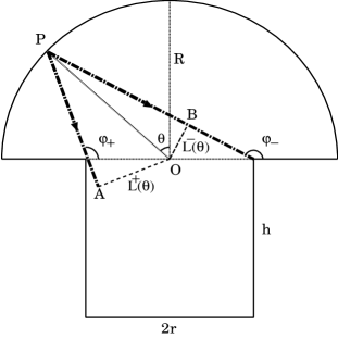
Figure 1: The shape of the board of the mushroom billiard (the solid lines), which consists of a half disk (the hat) and a rectangle (the foot). A point particle inside the board moves freely except for the elastic collisions with the walls. The absolute value of the angular momentum $|L|$ equals to the distance between the origin and the trajectory (See Sec. II A.). The boundaries $L^{\pm}(\theta)$ of the first escape domain $L^{-}(\theta)<L<L^{+}(\theta)$ are also displayed (See Sec. II B.).

II Poincaré Map and Its Inverse

The mushroom billiard is defined by the motion of a point particle on the billiard board depicted in Fig. 1. This board consists of a half disk (the hat) of radius $R$ and a rectangle (the foot) of width $r$ and height $h$ Bunimovich (2001). We use the polar coordinate $(u,\theta)$, and the Cartesian coordinate $(x,y)$; we set the origin as the center of the half disk in both cases. The angle variable $\theta$ is defined as the angle between the position vector of the point particle and the vertical line (See Fig. 1).

II.1 The definition of the Poincaré Map

We define a Poincaré surface at the arc of the semicircle $x^{2}+y^{2}=R^{2}(y\geq 0)$ with negative momentum of the radial direction, namely, just after the collision with the arc. For the coordinate of the Poincaré map, we use the angle $\theta$ and the associated angular momentum $L$. This Poincaré map $\Phi(L,\theta)$ is area-preserving; it can be proved through a direct calculation of the Jacobian of the map which equals to 1 everywhere. This coordinate system is slightly different from the Birkhoff coordinate, because the former is defined only on the arc, but the latter on the whole boundary of the billiard board.

We also set the kinetic energy as $v_{x}^{2}+v_{y}^{2}=1$. Although this setting is not essential, it is convenient to calculate the angular momentum $L$; the absolute value of the angular momentum $|L|$ equals to the distance from the origin to the trajectory. In Fig. 1, for example, if a point particle moves on the line $PA$ in the direction described in the figure, its angular momentum $L$ ($L>0$) equals the length of the segment $AO$ (the dashed line), and if a point particle moves on the line $PB$ in the direction described in the figure, the absolute value of the angular momentum $-L$ ($L<0$) equals the length of the segment $BO$ (the long-dashed line).

We display an example of the Poincaré surface in Fig. 2. The Poincaré map $\Phi(L,\theta)$ is defined on ${\mathcal{D}}=\{(L,\theta)\in[-R,R]\times[-\pi/2,\pi/2]\}$; the region $|L|<r$ is chaotic, and $|L|>r$ is torus. The Poincaré map is symmetric with respect to the origin $(L,\theta)=(0,0)$, i.e., $\Phi(L,\theta)=-\Phi(-L,-\theta)$. In the subsequent subsections, we will restrict the domain of the Poincaré map to the region of the negative momentum in order to simplify the analysis.

Figure 2: The Poincaré surface for $R=1$, $~{}r=0.5$ and $h=1$. The region $|L|<0.5$ is chaotic and the other integrable.

II.2 The first escape and re-injection domains

Let us consider a point $(L,\theta)$ on the Poincaré surface such that the original orbit of the billiard system (the continuous time flow) starting from this point escapes from the hat region to the foot without no collision. We define the first escape domain $\mathcal{D}_{1}$ as all such points on the Poincaré surface. The boundary of $\mathcal{D}_{1}$ can be calculated analytically as follows; fix the angle $\theta$ on the Poincaré surface, if the angular momentum $L$ satisfies the relation $L^{-}(\theta)<L<L^{+}(\theta)$, then $(L,\theta)\in{\mathcal{D}_{1}}$, where $L^{\pm}(\theta)$ are displayed in Fig. 1. More precisely, $L^{\pm}(\theta)$ are defined as

$$\begin{array}[]{lll}L^{\pm}(\theta)&=&\pm r\sin(\pi-\varphi_{\pm})\\[9.95863pt] &=&\pm rR\cos\theta~{}(R^{2}+r^{2}\mp 2Rr\sin\theta)^{-1/2},\end{array}$$ (3)

where the angles $\varphi_{\pm}$ are defined as in Fig. 1 and given by $\tan\varphi_{\pm}=R\cos\theta/(-R\sin\theta\pm r)$. Next, let us consider the the domain with negative angular momentum, $L^{-}(\theta)<L<0$; the positive domain $L>0$ can be treated in the same way because of the symmetry. Solving the equation $(L^{-}(\theta))^{2}>L^{2}$ in terms of $\theta$, the first escape domain for $L<0$ can be represented as

$${\mathcal{D}_{1}}=\{(L,\theta)\in{\mathcal{D}^{-}}~{}|~{}\theta^{-}(L)<\theta<\theta^{+}(L)\},$$ (4)

where ${\mathcal{D}^{-}}=\{(L,\theta)\in[-r,0]\times[-\pi/2,\pi,2]\}$ is the chaotic region with negative angular momentum and $\theta^{\pm}(L)$ are defined as

$$\theta^{\pm}(L)=\arcsin\left\{\displaystyle\frac{-L^{2}\pm\displaystyle\sqrt{L^{4}-L^{2}(R^{2}+r^{2})+r^{2}R^{2}}}{rR}\right\}.$$ (5)

The functions $\theta^{\pm}(L)$ defines the boundary of the first escape domain $\mathcal{D}_{1}$.

An orbit of the billiard flows starting from the first escape domain exits the hat region and stays in the foot for some times; and then it returns to the hat and reaches again to the Poincaré surface. We define the re-injection domain $\mathcal{D}_{\rm in}$ on the Poincaré surface as all such just returning points , more precisely, we define $\mathcal{D}_{\rm in}:=\Phi(\mathcal{D}_{1})$. $\mathcal{D}_{\rm in}$ can be derived in the same way as $\mathcal{D}_{1}$;

$${\mathcal{D}_{\rm in}}=\{(L,\theta)\in{\mathcal{D}^{-}}~{}|~{}\theta^{-}_{\rm in}(L)<\theta<\theta^{+}_{\rm in}(L)\},$$ (6)

where the boundary $\theta^{\pm}_{\rm in}(L)$ is defined by

$$\theta^{\pm}_{\rm in}(L)=\arcsin\left\{\displaystyle\frac{L^{2}\pm\displaystyle\sqrt{L^{4}-L^{2}(R^{2}+r^{2})+r^{2}R^{2}}}{rR}\right\}.$$ (7)

In Fig.3,  $\theta^{\pm}(L)$ and $\theta^{\pm}_{\rm in}(L)$ are displayed for $R=1$, $~{}r=0.5$ and $h>0$.

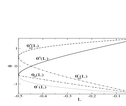
Figure 3: The boundaries $\theta^{+}(L)$ (the solid line), $\theta^{-}(L)$ (the dotted line), $\theta^{+}_{\rm in}(L)$ (the dashed line), $\theta^{-}_{\rm in}(L)$ (the dotted-and-dashed line), and $\theta_{0}(L)$ (the dotted-and-double-dashed line) are described. We set the system parameters as $R=1$, $~{}r=0.5$ and $h>0$. The only negative part of the angular momentum $L<0$ is displayed because the Poincaré surface is symmetric.

II.3 The inverse of the Poincaré map

When an orbit of the billiard flows collides with the boundary

$$W:=\{~{}(x,y)~{}|~{}x\in[-R,-r]\cup[r,R],~{}y=0\},$$ (8)

the angular momentum changes its sign. We should take into account the collisions with this boundary $W$, because we reduce the Poincaré map to the domain of negative momentum $L<0$. Let us consider the domain $\mathcal{D}^{-}\backslash{\mathcal{D}}_{\rm in}$ and its inverse image $\Phi^{-1}(\mathcal{D}^{-}\backslash{\mathcal{D}}_{\rm in})$. The original orbit $l$ (namely flow) connecting a point $(L,\theta)\in\mathcal{D}^{-}\backslash{\mathcal{D}}_{\rm in}$ and $\Phi^{-1}(L,\theta)\in\Phi^{-1}(\mathcal{D}^{-}\backslash{\mathcal{D}}_{\rm in})$ are classified into two classes for fixed $\theta$ (See Fig. 4(a).): when $L<L_{0}(\theta)$, the orbit $l$ is a line segment, namely there is no collision with the boundary $W$ and when $L>L_{0}(\theta)$, the orbit $l$ consists of two line segments, namely there is a collision with the boundary $W$. In Fig. 4(a), an orbit for the critical case $L=L_{0}(\theta)$ is displayed by the dashed line. We can define $L_{0}(\theta)$ by

$$L_{0}(\theta)=-R\cos(\psi-\theta),$$ (9)

where $\psi$ is defined as depicted in Fig. 4(a). Furthermore, using $~{}\tan\psi=\cos\theta/(1-\sin\theta)$, we have

$$L_{0}(\theta)=-R(2-2\sin\theta)^{-1/2}\cos\theta.$$ (10)

Solving the inequalities $L<L_{0}(\theta)$ and $L>L_{0}(\theta)$ in terms of $\theta$, we have the result: when $\theta<\theta_{0}(L)$ there is no collision with the boundary $W$, and when $\theta>\theta_{0}(L)$ there is a collision with the boundary $W$, where $\theta_{0}(L)$ is defined by

$$\theta_{0}(L)=\arcsin\left(\displaystyle\frac{2L^{2}}{R^{2}}-1\right).$$ (11)

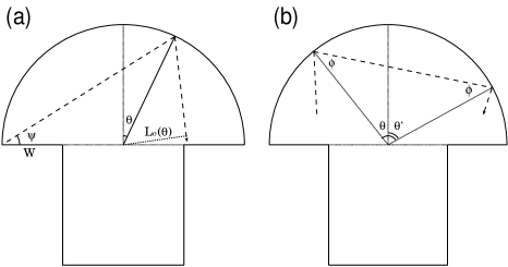
Figure 4: (a) A classification of orbits for fixed $\theta$ : if $L<L_{0}(\theta)~{}(<0)$ there is a collision with the wall $W$ and if $L_{0}(\theta)<L~{}(<0)$ there is no collision. Note that we consider only $L<0$. In the figure, we display the critical case $L=L_{0}(\theta)$ by the dashed line. (b) The inverse image of the Poincaré map, which is derived from $\theta=\theta^{\prime}+\pi-2\phi$ and $\phi=\arcsin|L/R|$.

Using these results and definitions, we can construct the inverse of the Poincaré map $\Phi^{-1}$ on $\mathcal{D}^{-}\backslash D_{\rm in}$ as follows (See Fig. 4(b)),

$$\Phi^{-1}(L,\theta)=\left\{\begin{array}[]{ll}\left(L,\theta+\pi-2\arcsin\left|\displaystyle\frac{L}{R}\right|\right),\\[14.22636pt] &{\rm if}~{}\theta<\theta_{0}(L)\\[14.22636pt] \left(L,\theta-2\arcsin\left|\displaystyle\frac{L}{R}\right|\right),&{\rm if}~{}\theta>\theta_{0}(L)\end{array}\right.$$ (15)

Notice that the angular momentum is unchanged by the collisions with the arc, and that we restrict the domain of the inverse map on the region $L<0$ by identifying the points $(-L,-\theta)$ with $(L,\theta)$ when the point particle collides with the wall $W$, i.e., when $\theta>\theta_{0}(L)$.

III The infinite partition

Using this inverse map $\Phi^{-1}$, we can define the $n$-th escape domain $\mathcal{D}_{n}$ recursively:

$${\mathcal{D}_{n}}=\Phi^{-1}({\mathcal{D}_{n-1}\backslash{\mathcal{D}_{\rm in}}}),~{}~{}~{}(n=2,3,\cdots).$$ (16)

Note that we should remove $\mathcal{D}_{\rm in}$ from $\mathcal{D}_{n-1}$ in the recursion relation Eq. (16), because the inverse image of the injection domain $\Phi^{-1}({\mathcal{D}_{\rm in}})$ equals to the first escape domain $\mathcal{D}_{1}$.

We restrict the parameters as $R=1$, $r=0.5$ and $h>0$ in the following and explicitly derive the boundaries of the $n$-th escape domain $\mathcal{D}_{n}$. First, we derive explicitly the first to fourth escape domains, in order to confirm that these four domains fill the domain $\mathcal{D}^{-}$ like Fig. 5(a) except for the three regions $E_{1},E_{2}$ and $E_{3}$. Then the boundaries of the $n$-th escape domain ($n\geq 5$) can be derived recursively.

Let us start with $n=2$ of Eq. (16). The domain ${\mathcal{D}_{1}/\mathcal{D}_{\rm in}}$ can be divided into three pieces:

$$\begin{array}[]{lll}{\mathcal{D}_{1}/\mathcal{D}_{\rm in}}&=&\{(L,\theta)~{}|~{}\theta^{-}(L)<\theta<\theta_{0}(L)\}\\[9.95863pt] &&\cup\{(L,\theta)~{}|~{}\theta_{0}(L)<\theta<\theta^{+}(L),~{}-r<L<L^{-}(0)\}\\[9.95863pt] &&\cup\{(L,\theta)~{}|~{}\theta_{0}(L)<\theta<\theta^{-}_{\rm in}(L),~{}L^{-}(0)<L<0\}.\end{array}$$ (20)

where $L^{-}(0)$ is defined by Eq. (3) (See also Fig. 5(b)). In Eq. (20), we abbreviate the expression $(L,\theta)\in{\mathcal{D}^{-}}$ to the one $(L,\theta)$ for simplicity; we use the same abbreviation in what follows. Let us represent the three sets on the right hand side as $\mathcal{F}^{1}_{1}$, $\mathcal{F}^{1}_{2}$, and $\mathcal{F}^{1}_{3}$, respectively; namely, $\mathcal{D}_{1}/\mathcal{D}_{\rm in}=\mathcal{F}^{1}_{1}\cup\mathcal{F}^{1}_{2}\cup\mathcal{F}^{1}_{3}$. These three sets are displayed in Fig. 5(b). Using these notations and the inverse map $\Phi^{-1}$ [Eq. (15)], the second escape domain $\mathcal{D}_{2}$ is given by

$$\begin{array}[]{lll}{\mathcal{D}_{2}}&=&\Phi^{-1}({\mathcal{D}_{1}/{\mathcal{D}_{\rm in}}})\\[9.95863pt] &=&\Phi^{-1}(\mathcal{F}^{1}_{1})\cup\Phi^{-1}(\mathcal{F}^{1}_{2})\cup\Phi^{-1}(\mathcal{F}^{1}_{3}).\end{array}$$ (23)

Let us denote the $\theta$ component of $\Phi^{-1}(L,\theta)$ as $\Psi^{L}(\theta)$, and inverse image of $\mathcal{F}_{1}^{1}$ as $\mathcal{F}^{2}_{1}\equiv\Phi^{-1}(\mathcal{F}^{1}_{1})$. Using these definitions, we have

$$\begin{array}[]{lll}\mathcal{F}^{2}_{1}&=&\{(L,\theta)~{}|~{}\Psi^{L}(\theta^{-}(L))<\theta<\Psi^{L}(\theta_{0}(L))\}\\[9.95863pt] &=&\{(L,\theta)~{}|~{}\theta^{-}(L)+\pi-2\arcsin\left|L\right|<\theta<\frac{\pi}{2})\},\end{array}$$ (26)

where the upper bound for $\theta$ is $\theta=\pi/2$. Note that the angular momentum $L$ is unchanged under the inverse map $\Phi^{-1}$. Similarly, we define the inverse image of $\mathcal{F}_{2}^{1}$ as $\mathcal{F}^{2}_{2}\equiv\Phi^{-1}(\mathcal{F}^{1}_{2})$, and we have

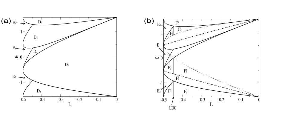
Figure 5: (a) The first to fourth escape domains $\mathcal{D}_{1}$–$\mathcal{D}_{4}$ are displayed. The second escape domain $\mathcal{D}_{2}$ is separated two parts. The remaining part consists of three pieces, which we define as $E_{0},E_{1}$ and $E_{2}$. (b) The regions $\mathcal{F}_{i}^{j}$ are displayed. The dotted line indicates the boundary of the re-injection domain.

$$\begin{array}[]{lll}\mathcal{F}^{2}_{2}&=&\{(L,\theta)~{}|~{}\Psi^{L}(\theta_{0}(L))<\theta<\Psi^{L}(\theta^{+}(L)),~{}-r<L<L^{-}(0)\}\\[9.95863pt] &=&\{(L,\theta)~{}|~{}-\frac{\pi}{2}<\theta<\theta^{+}(L)-2\arcsin\left|L\right|,~{}-r<L<L^{-}(0)\},\end{array}$$ (29)

where the lower bound for $\theta$ is $\theta=-\pi/2$. Finally, let us define the inverse image of $\mathcal{F}_{3}^{1}$ as $\mathcal{F}^{2}_{3}\equiv\Phi^{-1}(\mathcal{F}^{1}_{3})$, and we get

$$\begin{array}[]{lll}\mathcal{F}^{2}_{3}&=&\{(L,\theta)~{}|~{}\Psi^{L}(\theta_{0}(L))<\theta<\Psi^{L}(\theta^{-}_{\rm in}(L)),~{}L^{-}(0)<L<0\}\\[9.95863pt] &=&\{(L,\theta)~{}|~{}-\frac{\pi}{2}<\theta<\theta^{-}(L),~{}L^{-}(0)<L<0\}\end{array}$$ (32)

where we have used the relation $\theta^{-}(L)-\theta^{-}_{\rm in}(L)=-2\arcsin|L|$. In the Eq. (32), the lower bound for $\theta$ is $\theta=-\pi/2$; the upper is $\theta=\theta^{-}(L)$, which is equivalent to the lower bound of the domain $\mathcal{D}_{1}$. These three sets $\{\mathcal{F}^{2}_{1},\mathcal{F}^{2}_{2},\mathcal{F}^{2}_{3}\}$ are displayed in Fig. 5(b).

Next, we derive the third escape domain ${\mathcal{D}}_{3}$. It can be proved that $\mathcal{D}_{2}\cap\mathcal{D}_{\rm in}=\phi$, because the relation $\theta^{-}(L)+\pi-2\arcsin\left|L\right|>\theta_{\rm in}^{+}(L)$ holds. (See the lower bound of the domain $\mathcal{F}^{2}_{1}$ which is defined by the second line of the Eq. (26)). It follows that $\mathcal{D}_{3}=\Phi^{-1}(\mathcal{D}_{2})=\Phi^{-1}(\mathcal{F}^{2}_{1})\cup\Phi^{-1}(\mathcal{F}^{2}_{2})\cup\Phi^{-1}(\mathcal{F}^{2}_{3})$ by Eq. (16), where the three sets of the right hand side can be calculated, respectively, as

$$\begin{array}[]{lll}\Phi^{-1}(\mathcal{F}^{2}_{1})&=&\{(L,\theta)~{}|~{}\Psi^{L}(\theta^{-}(L)+\pi-2\arcsin|L|)<\theta<\Psi^{L}(\frac{\pi}{2})\}\\[9.95863pt] &=&\{(L,\theta)~{}|~{}\theta^{-}(L)+\pi-4\arcsin\left|L\right|<\theta<\frac{\pi}{2}-2\arcsin\left|L\right|\},\\[14.22636pt] \Phi^{-1}(\mathcal{F}^{2}_{2})&=&\{(L,\theta)~{}|~{}\Psi^{L}(-\frac{\pi}{2})<\theta<\Psi^{L}(\theta^{+}(L)-2\arcsin\left|L\right|),~{}-r<L<L^{-}(0)\}\\[9.95863pt] &=&\{(L,\theta)~{}|~{}\frac{\pi}{2}-2\arcsin\left|L\right|<\theta<\theta^{+}(L)+\pi-4\arcsin\left|L\right|,~{}-r<L<L^{-}(0)\},\\[14.22636pt] \Phi^{-1}(\mathcal{F}^{2}_{3})&=&\{(L,\theta)~{}|~{}\Psi^{L}(-\frac{\pi}{2})<\theta<\Psi^{L}(\theta^{-}(L)),~{}L^{-}(0)<L<0\}\\[9.95863pt] &=&\{(L,\theta)~{}|~{}\frac{\pi}{2}-2\arcsin\left|L\right|<\theta<\theta^{-}(L)+\pi-2\arcsin\left|L\right|,~{}L^{-}(0)<L<0\},\end{array}$$ (39)

where the relation $\Phi^{-1}(\mathcal{F}^{2}_{1})\subset\mathcal{D}_{\rm in}$ holds, because of the inequalities $\theta_{\rm in}^{+}(L)>\frac{\pi}{2}-2\arcsin\left|L\right|$ and $\theta^{-}(L)+\pi-4\arcsin|L|>\theta^{-}_{\rm in}(L)$. Therefor, the 4-th escape domain $\mathcal{D}_{4}$ is represented by $\mathcal{D}_{4}=\Phi^{-1}(\mathcal{D}_{3}/\mathcal{D}_{\rm in})=\Phi^{-1}(\mathcal{F}^{3}_{1})\cup\Phi^{-1}(\mathcal{F}^{3}_{2}),$ where we define

$$\begin{array}[]{lll}\mathcal{F}^{3}_{1}&=&\{(L,\theta)~{}|~{}\theta_{\rm in}^{+}(L)<\theta<\theta^{+}(L)+\pi-4\arcsin\left|L\right|,~{}-r<L<L^{-}(0)\}\\[9.95863pt] \mathcal{F}^{3}_{2}&=&\{(L,\theta)~{}|~{}\theta_{\rm in}^{+}(L)<\theta<\theta^{-}(L)+\pi-2\arcsin\left|L\right|,~{}L^{-}(0)<L<0\}\end{array}$$ (42)

These sets $\{\mathcal{F}^{3}_{1},\mathcal{F}^{3}_{2}\}$ are displayed in Fig. 5(b). Thus, the fourth escape domain $\mathcal{D}_{4}$ is given by the union of the following sets:

$$\begin{array}[]{lll}\Phi^{-1}(\mathcal{F}^{3}_{1})&=&\{(L,\theta)~{}|~{}\theta^{+}(L)<\theta<\theta^{+}(L)+\pi-6\arcsin\left|L\right|,~{}-r<L<L^{-}(0)\}\\[9.95863pt] \Phi^{-1}(\mathcal{F}^{3}_{2})&=&\{(L,\theta)~{}|~{}\theta^{+}(L)<\theta<\theta^{-}(L)+\pi-4\arcsin\left|L\right|,~{}L^{-}(0)<L<0\},\end{array}$$ (45)

where we have used the relation $\theta^{+}(L)-\theta^{+}_{\rm in}(L)=-2\arcsin|L|$. The lower bounds for $\theta$ of these two sets are $\theta=\theta^{+}(L)$; and the upper bounds of the set $\Phi^{-1}(\mathcal{F}^{3}_{2})$ is equivalent to the lower bound of $\mathcal{D}_{3}$.

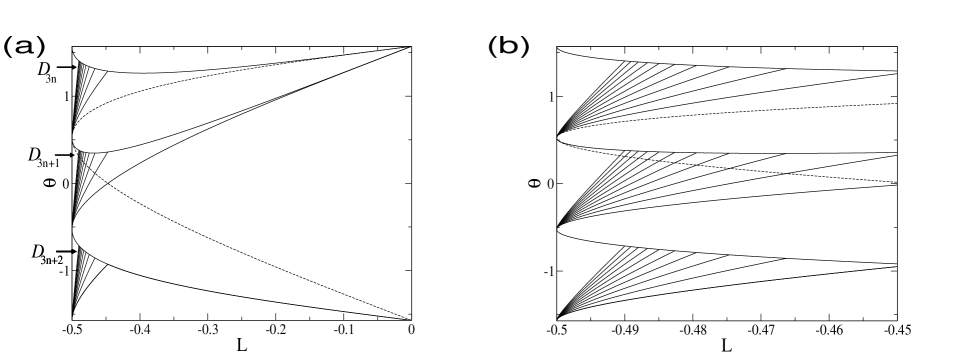
Figure 6: (a) The infinite partition constructed in terms of the escape time. The solid lines represents boundaries between regions of different escape times. The right hand side of the broken line is the injection domain. (b) A magnification of Fig. 6(a) in a neighborhood of the outermost tori ($L=-0.5$). The boundaries for the domains with the escape times longer than 32 are omitted.

From the above results, the domain ${\mathcal{D}^{-}}$ are covered by the four sets $\mathcal{D}_{1},\mathcal{D}_{2},\mathcal{D}_{3}$, and $\mathcal{D}_{4}$ except for the three regions $E_{0},E_{1}$, and $E_{2}$ as illustrated in Fig. 5(a)(b). The boundaries of the $n$-th escape domain ($n\geq 5$) can be obtained by recursively calculating the inverse mapping $\Phi^{-1}$ of the upper bound of the set $\Phi^{-1}(\mathcal{F}_{1}^{3})$, which is given by Eq. (45) as $\theta=\theta^{+}(L)+\pi-6\arcsin|L|$. Thus, let us define the boundary between the domains $\mathcal{D}_{3n+1}$ and $\mathcal{D}_{3(n+1)+1}$ as $\theta_{3n+1}(L)$ ($n\geq 1$), we have

$$\theta_{\rm 3n+1}(L)=\theta^{+}(L)+n\pi-6n\arcsin\left|L\right|$$ (46)

Similarly, defining the boundaries between $\mathcal{D}_{3n+2}$ and $\mathcal{D}_{3(n+1)+2}$ as $\theta_{3n+2}(L)$, and between $\mathcal{D}_{3n}$ and $\mathcal{D}_{3(n+1)}$ as $\theta_{3n}(L)$ , we have

$$\begin{array}[]{lll}\theta_{\rm 3n+2}(L)&=&\theta^{+}(L)+n\pi-2(3n+1)\arcsin\left|L\right|,\\[9.95863pt] \theta_{\rm 3n}(L)&=&\theta^{+}(L)+n\pi-2(3n-1)\arcsin\left|L\right|\end{array}$$ (49)

In Figs. 6(a) and (b), we depict these boundaries up to $n=31$.

IV The escape time distribution

Figure 7: The cumulative distributions of the escape times for discrete time (the solid line) and for continuous time (the dotted line) in log-log form. The dashed line is the analytical result $F(t)\sim 1/t^{2}$. The inset is a magnification of the discrete time case, which shows a clear stepwise structure.

Finally, we derive a scaling property of the escape time distribution $f_{\rm esc}(n)$ approximately. The escape time is defined by the number of collisions with the arc of the semicircle just after an orbit enters the hat region until it escapes from there.

Since the Poincaré map is area-preserving, which is the universal property of the Poincaré map of the Hamiltonian systems, the physically natural invariant measure of the Poincaré map is the Lebesgue measure. Thus the probability that the escape time equals $n$ is given by the Lebesgue measure $S_{n}^{\rm in}$ of the region $\mathcal{D}_{n}\cap\mathcal{D}_{\rm in}$, that is $f_{\rm esc}(n)=S_{n}^{\rm in}$. Note that $S_{3n}^{\rm in}=S_{3n-1}^{\rm in}=0~{}(n=2,3,\cdots)$ and thus only $S_{3n+1}^{\rm in}~{}(n=1,2,\cdots)$ has finite values (See Fig. 6(a)(b).).

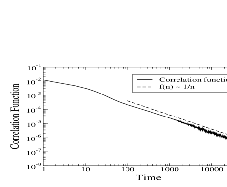
Figure 8: Auto correlation function of the absolute value of the angular momentum $|L|-\langle|L|\rangle$ (the solid line) in log-log form, where $\langle\cdot\rangle$ means the ensemble average in terms of the Lebesgue measure in the chaotic domain. The broken line represents a function $f(n)\sim 1/n$, which is a guide to see.

Let us derive the cross points of the lines $\theta_{3n+1}(L)=\theta^{+}(L)+n\pi-6n\arcsin\left|L\right|$ [Eq. (46)] and $\theta(L)=0$. Using the Taylor expansions $\arcsin x\approx\pm\frac{\pi}{6}+\frac{2}{\sqrt{3}}\left(x\mp\frac{1}{2}\right)$   (as $x\approx\pm\frac{1}{2}$), we have

$$\begin{array}[]{lll}\theta_{3n+1}(L)&\approx&\\[9.95863pt] &&-\displaystyle\frac{\pi}{6}+\displaystyle\frac{2}{\displaystyle\sqrt{3}}(3n+1)(2L+1)+\displaystyle\sqrt{2}(2L+1)^{\frac{1}{2}},\end{array}$$ (52)

as $n\to\infty$. Setting this to $0$, and solving in terms of $L$, we have $2L+1\sim\frac{1}{3n+1}\sim\frac{1}{n}$. Thus we find the width of the $(3n+1)$-th escape domain is proportional to $1/n^{2}$. It follows that the area of the $n$-th escape domain $S_{n}$ behaves as

$$S_{n}\sim\displaystyle\frac{1}{n^{2}},$$ (53)

as $n\to\infty$. Note that $S_{3n+1}=S_{3n}=S_{3n-1}$ for $n=2,3,\cdots$, because the domains $\mathcal{D}_{3n}$ and $\mathcal{D}_{3n-1}$ has no intersection with the domain $\mathcal{D}_{\rm in}$. The Eq. (53) means the fact that the partition constructed in the previous section is infinite. Finally, we get

$$S_{3n+1}^{\rm in}=S_{3n+1}-S_{3n+4}\sim\displaystyle\frac{1}{n^{3}},$$ (54)

as $n\to\infty$. And, as mentioned above, the equations $S_{3n}^{\rm in}=S_{3n-1}^{\rm in}=0$ hold. This power law perfectly agrees with the numerical results shown in Fig. 7, where the cumulative distribution

$$F_{\rm esc}(n):=\sum_{j=n+1}^{\infty}f_{\rm esc}(j)$$ (55)

is plotted by the solid line. Note that this numerical result have already been reported by Altmann et. al.Altmann et al. (2005). In the inset, a magnification is displayed, which shows a clear stepwise structure with decreases exactly at $n=3k+1~{}(k=1,2,\cdots)$. This implies that $f_{\rm esc}(3k)=f_{\rm esc}(3k+2)=0$, and that the only $f_{\rm esc}(3k+1)$ have finite values $(k\geq 2)$. Thus, these results also agree with the analytical results.

V Concluding remarks

In conclusion, we have derived the escape time distribution by constructing the infinite partition in terms of the escape times. Note that, however, the escape ’time’ in this paper is the number of collision until the particle escapes. Thus the escape time of the continuous time flow might be slightly different from ours. But the scaling exponents should be the same, because the flight time of the chaotic orbits between collisions in the hat region is non-vanishing. This is confirmed numerically and the result is displayed in Fig. 7 which shows the agreement of the scaling exponents of these two distributions.

There are several points that should be verified in future studies. First, the correlation functions of this system exhibits power law behavior (Fig. 8, see also Bunimovich (2001)), and it is expected that there are relations between the scaling exponent of the escape time distributions and the correlation functions. Second, it is important to elucidate whether the results in this paper is general or not for other parameter values $R\neq 2r$. Third, it is also important to consider which property of the mushroom billiard is the universal features of the mixed type Hamiltonian systems.