Interactions of Parametrically Driven Dark Solitons. I:
Néel-Néel and Bloch-Bloch interactions

Abstract

We study interactions between the dark solitons of the parametrically driven nonlinear Schrödinger equation, Eq.(1). When the driving strength, $h$, is below $\sqrt{\gamma^{2}+1/9}$, two well-separated Néel walls may repel or attract. They repel if their initial separation $2z(0)$ is larger than the distance $2z_{u}$ between the constituents in the unstable stationary complex of two walls. They attract and annihilate if $2z(0)$ is smaller than $2z_{u}$. Two Néel walls with $h$ lying between $\sqrt{\gamma^{2}+1/9}$ and a threshold driving strength $h_{sn}$ attract for $2z(0)<2z_{u}$ and evolve into a stable stationary bound state for $2z(0)>2z_{u}$. Finally, the Néel walls with $h$ greater than $h_{sn}$ attract and annihilate — irrespective of their initial separation. Two Bloch walls of opposite chiralities attract, while Bloch walls of like chiralities repel — except near the critical driving strength, where the difference between the like-handed and oppositely-handed walls becomes negligible. In this limit, similarly-handed walls at large separations repel while those placed at shorter distances may start moving in the same direction or transmute into an oppositely-handed pair and attract. The collision of two Bloch walls or two nondissipative Néel walls typically produces a quiescent or moving breather.

I Introduction

This paper deals with the parametrically driven, repulsive nonlinear Schrödinger (NLS) equation:

$$i\partial_{t}\Psi+{\textstyle\frac{1}{2}}\partial_{X}^{2}\Psi+\Psi-|\Psi|^{2}\Psi=h\Psi^{*}-i\gamma\Psi.$$ (1)

Here $h$ is the strength of the parametric driving and $\gamma$ is the damping coefficient. In the absence of damping, i.e. when $\gamma=0$, this equation has the same stationary Bloch- and Néel-wall solutions as the (2:1)-resonantly forced Ginzburg-Landau equation and the relativistic Montonen-Sarker-Trullinger-Bishop model Sarker ; Montonen ; Niez ; Niez2 . However, unlike the Ginzburg-Landau and the relativistic model, where only one of these solutions (the Bloch wall) is linearly stable in their region of coexistence, the NLS equation exhibits Bloch-Néel bistability. Furthermore, both domain-wall solutions of the NLS (also known as dark solitons or kinks) can move with constant velocity, and the moving walls also turn out to be linearly stable OurPaper . This multistability is a rare phenomenon and leads one to wonder about the outcome of the soliton-soliton interaction. The problem that is of ultimate interest to a physicist, is formulated as follows: Given an initial configuration of many different walls, will the asymptotic solution, as $t\rightarrow\infty$, consist of predominantly Bloch walls, Néel walls or possibly some other, more complicated, structures? Will the walls form widely spaced, equidistant lattices, or tightly bound clusters? In this paper we make the first step towards answering these questions.

When $\gamma\neq 0$, equation (1) still has a dark soliton solution (in the form of the Néel wall); this solution was shown to be stable for all $\gamma$ OurPaper . Our analysis of soliton interactions will naturally include the case of nonzero damping, especially in view of the wide range of applications of Eq.(1).

Equation (1) was indeed derived in a broad variety of physical situations. In fluid dynamics, the repulsive (“defocusing”) parametrically driven NLS describes the amplitude of the water surface in a vibrated channel with large width-to-depth ratio Elphick_Meron ; Larraza ; Chen . (The case of the small width-to-depth ratio gives rise to the attractive NLS Elphick_Meron ; Larraza ; Chen .) The same equation arises as an amplitude equation for the upper cutoff mode in a chain of parametrically driven, damped nonlinear oscillators. In the optical context, it was derived for the doubly resonant $\chi^{(2)}$ optical parametric oscillator in the limit of large second-harmonic detuning Trillo . Next, stationary solutions of Eq.(1) with $\gamma=0$ minimise the Ginzburg-Landau free energy of the anisotropic $XY$-model. Here $F=\int{\cal F}d{X}$, where

$${\cal F}={\textstyle\frac{1}{2}}(\partial_{X}{\bf M})^{2}-(1+h){\bf M}^{2}+{\textstyle\frac{1}{2}}{\bf M}^{4}+2hM_{y}^{2}+{\cal F}_{0},$$

and ${\bf M}(X)=(0,M_{y},M_{z})$ is the magnetisation vector whose nontrivial components serve as the real and imaginary parts of the complex field $\Psi(X)$ in (1): $\Psi=M_{y}+iM_{z}$. This model appeared in studies of stationary domain walls in easy-axis ferromagnets near the Curie point XY . Nonstationary magnetisation configurations were considered in the overdamped limit: $\Psi_{t}=-\delta F/\delta\Psi^{*}$ Coullet . The damped hamiltonian dynamics $\Psi_{t}=-i\delta F/\delta\Psi^{*}-\gamma\Psi$ provides a sensible alternative; this is precisely our equation (1).

Finally we note that Eq.(1) also arises in a completely different magnetic context — that of a weakly anisotropic easy-plane ferromagnet in a constant external magnetic field OurPaper . Here, the external field (chosen parallel to the $z$-axis) forces the magnetisation to be almost homogeneous, and Eq.(1) describes small deviations $\epsilon\Psi=M_{x}+iM_{y}$ from the uniform magnetisation ${\bf M}\approx(0,0,1)$. (Here $\epsilon$ is a small parameter.) In the $XY$-model, on the other hand, Eq.(1) governs the magnetisation vector itself.

The literature devoted to the interactions of dark solitons and kinks is quite extensive (although perhaps not as vast as for bright solitons and pulses). Kinks are known to attract antikinks in real-valued, single-component Klein-Gordon equations, such as the sine-Gordon and $\phi^{4}$-theory RajKink , with and without damping terms KawOhta . The same is true for kinks of the real Ginzburg-Landau equations $u_{t}=u_{xx}-V^{\prime}(u)$ KawOhta . These results admit simple interpretations; the kink-antikink pair converges in order to minimise its total energy in the former case, and to minimise the value of its Lyapunov functional in the latter. Next, the dark solitons of the (undriven) NLS equations are known to repel ZakShab ; KivsharReview . This can also be understood as an attempt to minimise the energy of the pair, at the expense of the gradient of the phase. Proceeding to the domain-wall solutions of the parametrically driven Ginzburg-Landau equation

$$\partial_{t}\Psi={\textstyle\frac{1}{2}}\partial_{X}^{2}\Psi+\Psi-|\Psi|^{2}\Psi-h\Psi^{*},$$ (2)

the Bloch wall and antiwall of opposite chiralities were shown to attract, while those of like chiralities repel Korz ; Tutu . (Here $h<\frac{1}{3}$, the region of stability of Bloch walls.) The Néel wall and antiwall always repel in their stability region ($h>\frac{1}{3}$) Korz . Unlike the case without driving, the interpretation of these interactions is not straight-forward though.

As for the driven NLS equation, the behaviour of its Bloch and Néel walls is even less predictable at the intuitive level, while the variety of possible interacting partners is much wider due to the multistability. We will see that the interaction pattern is quite complicated indeed. The character of interaction (repulsion vs attraction) will depend both on the driving strength and the interwall separation. We will also show that it is influenced by stationary complexes of walls, stable and unstable.

This paper constitutes the first part of our project; here, we restrict ourselves to interactions of the walls of the same type, i.e. Néel-Néel and Bloch-Bloch interactions. The analysis of the nonsymmetric situations, i.e. Néel-Bloch interactions, requires a different mathematical formalism and will be presented separately. (See the following publication BW2 .)

The dynamics of the repelling solitons is, in a sense, trivial: if the walls are initially at rest, they will simply diverge to the infinities. Less obvious is what the collision of two attracting walls will result in. The study of the asymptotic (as $t\to\infty$) attractors arising in the parametrically driven NLS constitutes the second objective of our work. We will show that if the dynamics are dissipative, then, depending on the strength of the driving, colliding walls either annihilate or form a stable stationary bound state. In contrast to this, undamped collisions will be found to always produce a breather, a spatially localised, temporally oscillating structure. Depending on the initial conditions, the breather propagates or remains motionless, and in either case is found to persist indefinitely.

The outline of this paper is as follows. The two fundamental solutions of Eq.(1), the Bloch and Néel wall, are introduced in the next section. For the analysis of the Bloch-Bloch and Néel-Néel interaction we use the variational method, under the assumption of well-separated walls. The method is detailed in section III and the resulting finite-dimensional systems are analysed in sections IV, VII, and VIII. Section IV deals with the Néel walls; section VII is devoted to the Bloch walls of the opposite chirality, while the like-chirality walls are examined in section VIII. The conclusions of the variational analysis have been verified in direct numerical simulations of the full partial differential equation. The numerical simulations allow to advance beyond the limit of well-separated walls; in particular, we use this approach to examine the outcome of soliton collisions. We have allocated a separate section (section VI) to the Néel-Néel simulations while the Bloch-Bloch simulations are reported in sections VII and VIII, along with the corresponding variational results. The nontrivial attractors mentioned above — the stationary bound state in the case of dissipative dynamics, and the breather in the undamped system — are further investigated in sections V and IX, respectively. Finally, the main results of this work are summarised in section X.

II Dark solitons: preliminaries

Dark solitons are localised patches of low intensity ($|\Psi|^{2}\ll 1$) in a high intensity background ($|\Psi|^{2}=\mathcal{O}(1)$). The admissible backgrounds are described by the stationary, spatially homogeneous nonzero solutions of Eq.(1),

$$\Psi^{(\pm)}_{\mbox{flat}}=iA_{\pm}e^{i\theta_{\pm}},$$ (3)

where

$$A_{\pm}=\sqrt{1\pm\sqrt{h^{2}-\gamma^{2}}},$$

$$2\theta_{+}=\arcsin{\frac{\gamma}{h}},\quad 2\theta_{-}=\pi-\arcsin{\frac{\gamma}{h}}.$$ (4)

As one can easily check, for $h\leq\gamma$ the zero solution is the only stable background and so dark solitons can only exist for $h>\gamma$; this is the condition we are implicitly assuming in this paper. It can be shown that $\Psi^{(+)}_{\mbox{flat}}$ is stable for all values of $h>\gamma$ while $\Psi^{(-)}_{\mbox{flat}}$ is always unstable. We will only consider dark solitons existing over the stable background so that all solutions obey $|\Psi|^{2}\rightarrow A_{+}^{2}$ as $|X|\rightarrow\infty$. Accordingly, $A$ stands for $A_{+}$ and $\theta$ for $\theta_{+}$ for the rest of the paper.

It will be convenient to transform Eq.(1) so that the asymptotic solution is independent of $h$ and $\gamma$. To this end, we set

$$\Psi(X,t)=iAe^{i\theta}\psi(x,t),\quad x=AX.$$ (5)

(We have also rescaled the spatial dependence for later convenience.) Under this transformation, Eq.(1) becomes

$$i\psi_{t}+{\textstyle\frac{A^{2}}{2}}\psi_{xx}-A^{2}|\psi|^{2}\psi+\psi+(A^{2}-1)\psi^{*}+i\gamma(\psi-\psi^{*})=0.$$ (6)

This is the form of the parametrically driven, damped NLS that we will be working with in this paper. The stable background solutions of Eq.(6) are simply $\psi_{\mbox{flat}}=\pm 1$.

Solutions to Eq.(6) with $|\psi|\to 1$ as $|x|\to\infty$ can either be topological $\left[\psi(-\infty)=-\psi(\infty)\right]$ or nontopological $\left[\psi(-\infty)=\psi(\infty)\right]$. Eq.(6) has two explicit topological solitons. The first is the Néel, or Ising, wall XY ; Raj ; Niez ; Niez2 ; Elphick_Meron :

$$\psi_{N}(x)=\tanh(x),$$ (7)

named after the Néel wall in magnetism, which is a domain wall with the magnitude of the magnetisation vector vanishing at its centre. The second topological solution, which exists only for $\gamma=0$, is usually referred to as the Bloch wall Sarker ; Montonen ; Niez ; Niez2 :

$$\psi_{B}(x)=\tanh(Bx)\pm i\kappa_{0}\,\mbox{sech}(Bx).$$ (8)

(In magnetism, a Bloch wall is a domain wall connecting the two domains smoothly, with the magnetisation vector remaining nonzero everywhere.) In Eq.(8),

$$B=\frac{2\sqrt{A^{2}-1}}{A}=\sqrt{\frac{4h}{1+h}}$$

and

$$\kappa_{0}=\frac{\sqrt{4-3A^{2}}}{A}=\sqrt{\frac{1-3h}{1+h}}.$$ (9)

The solutions obtained by multiplying $\psi_{N}$ and $\psi_{B}$ by $(-1)$ will be called antiwalls, or antikinks.

The Bloch wall (8) exists in two chiralities. In the Bloch wall with positive imaginary part, the phase of the complex field $\psi(x)$ decreases (that is, the point on the unit circle moves clockwise) as $x$ varies from $-\infty$ to $+\infty$. By analogy with the right-hand rule of circular motion, we refer to this wall as the right-handed Bloch wall. The phase of the Bloch wall with negative imaginary part increases as $x$ increases (that is, the phase vector rotates counter-clockwise). This corresponds to a left-handed sense of rotation, so that this wall will be called the left-handed Bloch wall. The antiwall obtained by multiplying $\psi_{B}$ by $-1$ has obviously the same chirality as its parent wall, $\psi_{B}$. Regardless of their chirality, Bloch walls only exist for $h<\frac{1}{3}$.

In Ref.OurPaper , it was proved that the Néel wall is stable for all $h>\gamma$. The stability of the Bloch wall in its entire domain of existence was demonstrated numerically OurPaper .

Examples of nontopological dark solitons are given by stationary complexes, or bound states, of domain walls. These can be formed by two dissipative Néel walls, or by a Bloch and Néel wall — in the undamped situation. (See OurPaper ; OurPaper2 .) In condensed matter physics, these nontopological solitons describe bubbles of one thermodynamic phase in another one bubbles . Accordingly, we will occassionally be referring to bound states of domain walls as solitonic bubbles.

III Interactions between the walls: the method

In this paper, we will be paying special attention to the simplest situation where the interacting walls are initially at rest. Choosing the origin of the coordinate axis midway between two Bloch or two Néel walls, one can verify that the subsequent evolution will preserve this symmetric arrangement (see below). A symmetric pair of well separated walls can be approximated by a product function

$$\psi=\varphi_{1}(x,t)\varphi_{2}(x,t),$$ (10a)

where $$\varphi_{1} \varphi_{2}$$ and represent the individual walls in the pair:

$$\varphi_{1}(x,t)=\tanh{[{\cal B}(x+z)]}-i\kappa_{1}\mbox{sech}[{\cal B}(x+z)],$$ (10b)

$$\varphi_{2}(x,t)=\tanh{[{\cal B}(x-z)]}+i\kappa_{2}\mbox{sech}[{\cal B}(x-z)].$$ (10c)

In Eq.(10), $\kappa_{1}$ and $\kappa_{2}$ are time-dependent parameters accounting for the deformation of the walls due to their interaction. The variable $z=z(t)$ gives half the distance between the walls; without loss of generality, we take $z$ to be positive. Finally, the constant ${\cal B}$ characterises the width of the walls (${\cal B}=B$ for Bloch walls and ${\cal B}=1$ for Néel walls).

Our analysis is based on the variational method. For this method, we substitute the Ansatz (10) into the action integral that gives rise to Eq.(6):

$${\cal S}=\int\mathcal{L}e^{2\gamma t}\ dt,$$ (11)

where

$$\mathcal{L}=\mbox{Re}\int\left\{i\psi_{t}\psi^{*}-\frac{A^{2}}{2}\left|\psi_{x}\right|^{2}-\frac{A^{2}}{2}\left|\psi\right|^{4}+\left|\psi\right|^{2}+\frac{A^{2}-1}{2}\left[\psi^{2}+(\psi^{*})^{2}\right]+\frac{i\gamma}{2}\left[\psi^{2}-(\psi^{*})^{2}\right]-\frac{A^{2}}{2}\right\}dx.$$ (12)

In what follows we introduce a small parameter $\epsilon=e^{-2{\cal B}z}$. Integrating off the explicit $x$-dependence in (12), produces a finite-dimensional lagrangian

$${\cal L}=T-V,$$ (13a)

where

$$T=-\pi\dot{z}(\kappa_{1}+\kappa_{2})\left[1-2(1-\kappa_{1}\kappa_{2})(\epsilon-2\epsilon^{2})\right]$$

$$-\frac{2\pi}{\cal B}(\epsilon-4\epsilon^{2})\left[\dot{\kappa_{1}}(1-\kappa_{2}^{2})+\dot{\kappa_{2}}(1-\kappa_{1}^{2})\right],$$ (13b)

and

$$V=\frac{A^{2}{\cal B}^{2}+8A^{2}-12}{3{\cal B}}(\kappa_{1}^{2}+\kappa_{2}^{2})+\frac{2A^{2}}{3{\cal B}}(\kappa_{1}^{4}+\kappa_{2}^{4})+8\left[(4A^{2}-A^{2}{\cal B}^{2}-4)z-\frac{4}{{\cal B}}(A^{2}-1)\right]\epsilon\kappa_{1}\kappa_{2}\\ +\frac{8}{3{\cal B}}\epsilon^{2}\left[2A^{2}(4{\cal B}^{2}-7)+(30A^{2}-5A^{2}{\cal B}^{2}-12)(\kappa_{1}^{2}+\kappa_{2}^{2})\right.\\ \left.+2A^{2}({\cal B}^{2}-11)\kappa_{1}^{2}\kappa_{2}^{2}-4A^{2}(\kappa_{1}^{4}+\kappa_{2}^{4})+4A^{2}(\kappa_{1}^{2}+\kappa_{2}^{2})\kappa_{1}^{2}\kappa_{2}^{2}\right]\\ +16\epsilon^{2}z\left[2A^{2}(1-{\cal B}^{2})+(A^{2}{\cal B}^{2}-6A^{2}+4)(\kappa_{1}^{2}+\kappa_{2}^{2})+2A^{2}\kappa_{1}^{2}\kappa_{2}^{2}\right]+\frac{4\pi\gamma}{{\cal B}}\epsilon(1-4\epsilon)(\kappa_{1}+\kappa_{2})(1+\kappa_{1}\kappa_{2}).$$ (13c)

[In (13b), the overdot indicates differentiation with respect to $t$.] The stationary action principle $\delta{\cal S}=0$ yields then the Euler-Lagrange equations for $\kappa_{1,2}$ and $z$. In deriving (13b)-(13c) we neglected all powers of $\epsilon$ higher than $\epsilon^{2}$. One can readily check that such terms would produce only higher-order corrections in the resulting equations of motion.

Some comments must be made regarding the Ansatz (10). After a variational Ansatz has been substituted in the corresponding field Lagrangian and the $x$-dependence integrated away, all dynamical variables (or possibly their combinations) can be grouped into canonically-conjugate pairs. (See MalomedReview for review and references.) In particular, if the waveform consists of two solitary waves and the separation between two constituents, $2z$, is chosen as one of the variables, the conjugate momentum is the phase gradient. This fact is well known in the case where the constituents are bell-shaped (“bright”) solitons (see e.g. YanMei ; Variational ). That it remains true in a more general situation can be seen from an analogy with quantum mechanics where the momentum of the system is given by an eigenvalue of the operator $\frac{1}{i}\partial_{x}$. (Since the eigenvalue has to be real, the operator acts just on the phase of the eigenfunction while the modulus is taken to be constant.) Another simple analogy arises if we write $\psi=\sqrt{\rho}e^{i\chi}$; this polar decomposition casts Eq.(1) with $h=\gamma=0$ in the form of equations of gas dynamics, where $\rho$ is the density of the gas and $\partial_{x}\chi$ is its velocity, proportional to the momentum.

In the case of bright solitons, each constituent soliton in the Ansatz is usually multiplied by $e^{ik(x\pm z)}$ (see e.g. YanMei ; Variational ); then, the momentum conjugate to $z$ is $k$. However, in the case of kinks this simple recipe would violate the boundary conditions at infinity. For this reason we have introduced the phase gradient by allowing the imaginary parts $\kappa_{1,2}\,\mbox{sech}\,[{\cal B}(x\pm z)]$ of the kinks to be variable. The imaginary parts decay as $|x|\to\infty$ and therefore making them variable is compatible with the boundary conditions. Below, we will show that $\kappa_{1}$ and $\kappa_{2}$ are indeed momenta canonically conjugate to $z$.

Another reason for introducing the phase gradient in this way is a simple interpretation of the finite-dimensional momenta $\kappa_{1}$ and $\kappa_{2}$ in terms of the original fields $\psi(x,t)$. Indeed, these variables coincide, modulo a numerical coefficient, with the field momenta of the two walls. The field momentum integral has the form

$$P=\frac{i}{2}\int\left(\psi_{x}^{*}\psi-\psi_{x}\psi^{*}\,\right)dx.$$ (14)

For the undamped NLS [equation (6) with $\gamma=0$], the integral (14) is conserved. The field momentum of the Néel wall (7) equals zero, while that of the Bloch wall (8) is given by $P_{\rm B}=\mp\pi\kappa_{0}$. [The same sign convention is used here as for Eq.(8) — the top sign applies for the right-handed wall, while the bottom sign corresponds to the left-handed wall.] It is not difficult to check that the field momenta of the perturbed walls $\varphi_{1}$ and $\varphi_{2}$ in the configuration (10) are $P[\varphi_{1}]=\pi\kappa_{1}$ and $P[\varphi_{2}]=-\pi\kappa_{2}$.

In symmetric situations that we are concerned with, the variables $\kappa_{1}$ and $\kappa_{2}$ (both of which are conjugate to the same coordinate variable $z$) will eventually turn out to be related due to the equations of motion. The calculations simplify, however, if this relationship is established yet at the level of the lagrangian (13), that is, before the equations of motion have been derived.

The relationship between $\kappa_{1}$ and $\kappa_{2}$ depends on the type of walls being considered. If the initial configuration consists of two well-separated Néel walls at rest, or two quiescent distant Bloch walls of opposite chirality, we have a symmetry $\psi(x,0)=\psi(-x,0)$. Since equation (6) is parity-invariant, the subsequent evolution will preserve this symmetry. Substituting the Ansatz (10) into $\psi(x,t)=\psi(-x,t)$, we get $\kappa_{1}=\kappa_{2}$. The initial value of $\kappa(t)$ should be chosen close to zero for Néel walls and close to $\pm\kappa_{0}$ for Bloch walls [with the sign of $\kappa(0)$ depending on whether the wall placed on the right is right- or left-handed.]

If the initial configuration consists of two quiescent Bloch walls of like chirality, the relationship between $\kappa_{1}$ and $\kappa_{2}$ is not so trivial to establish. The reason is that equation (6) does not preserve the symmetry $\psi^{*}(x,0)=\psi(-x,0)$ of the initial condition. In this case we have to appeal to the field-momentum considerations rather than symmetries. Substituting the Ansatz (10) into the integral (14), we find that $P[\psi]=\pi(\kappa_{1}-\kappa_{2})[1+\mathcal{O}(e^{-2{\cal B}z})]$. On the other hand, the total momentum of two like-chirality walls which are initially at rest and far away from each other, should be near $\mp 2\pi\kappa_{0}$. Therefore, for moving walls the quantity $\kappa_{1}-\kappa_{2}$ must not be different from $\mp 2\kappa_{0}$ by more than ${\cal O}(e^{-2Bz})$. This is accomplished by letting $\kappa_{1}=\mp\kappa_{0}+q(t)$ and $\kappa_{2}=\pm\kappa_{0}+q(t)$. When $z$ is large, the perturbation $q(t)$ is small — but not necessarily as small as $\epsilon$.

The Euler-Lagrange equations corresponding to Eqs.(11),(13) are

$$\frac{\partial T}{\partial\kappa}-\frac{\partial V}{\partial\kappa}-\frac{d}{dt}\frac{\partial T}{\partial\dot{\kappa}}-2\gamma\frac{\partial T}{\partial\dot{\kappa}}=0,$$ (15a)

and

$$\frac{\partial T}{\partial z}-\frac{\partial V}{\partial z}-\frac{d}{dt}\frac{\partial T}{\partial\dot{z}}-2\gamma\frac{\partial T}{\partial\dot{z}}=0.$$ (15b)

In Eq.(15a), we assumed the situation of $\kappa_{1}=\kappa_{2}\equiv\kappa$ (that is, two Néel or two oppositely-handed Bloch walls). In the other case, i.e. when we have two Bloch walls of like chirality, $\kappa$ should be replaced by $q$ in Eq.(15a). The integrals $T$ and $V$ can both be found explicitly and simplified assuming wide separation of the walls.

Finally, we note that the variational method is not well suited for the analysis of the Bloch-Néel interaction. The reason for this is that the Bloch and Néel walls have different widths, leading to terms in the Lagrangian which are not periodic along the imaginary axis on the plane of complex $x$; as a result, the Lagrangian cannot be obtained in closed form. (When the walls have the same width, the integrals can all be evaluated by integration along the rectangular contour with one side on the real axis and the other on the line $\mbox{Im}\,{x}=\pi/\cal B$.) Consequently, we had to resort to a different approach for the analysis of the Néel-Bloch interaction (see paper II of this project BW2 .) The resulting phenomenology is also very different BW2 .

IV Two Néel walls

In this case, we let ${\cal B}=1$ and $\kappa_{1}=\kappa_{2}\equiv\kappa$. In equations (15) we discard products of powers of small quantities $\epsilon$ and $\kappa$ for which there are larger counterparts. For instance, we drop a term proportional to $\epsilon^{2}\kappa$ from an equation which already has a term $\epsilon\kappa$ with a nonsmall coefficient. Here we keep in mind that in some cases the damping $\gamma$ and the difference $|A^{2}-\frac{4}{3}|$ can be small parameters, hence we cannot drop $\epsilon^{2}\kappa$ in favour of the term $\gamma\epsilon\kappa$ or $(A^{2}-\frac{4}{3})\epsilon\kappa$. With these simplifications, equations (15a)-(15b) take the form

$$\pi\dot{\epsilon}=12\left(A^{2}-\frac{4}{3}\right)\kappa\epsilon$$

$$+32\pi\gamma\epsilon^{2}\kappa^{2}+\frac{16}{3}A^{2}\kappa^{3}\epsilon-64(A^{2}-1)\kappa\epsilon^{2},$$ (16a)

$$\pi(\dot{\kappa}+2\gamma\kappa)=32A^{2}\epsilon^{2}$$

$$-24\left(A^{2}-\frac{4}{3}\right)\kappa^{2}\epsilon z+32(A^{2}-1)\epsilon\kappa^{2}.$$ (16b)

The subsequent analysis depends on the relation between the damping and driving in the system.

IV.1 $\gamma={\cal O}(1)$

First we consider the case where $\gamma$ is not small. Assume, in addition, that $A^{2}$ is not close to $\frac{4}{3}$. (Later in this subsection we will explore the situation where $|A^{2}-\frac{4}{3}|$ is small.) In this case the terms in the second lines of (16a) and (16b) are smaller than those in the first lines and can be neglected. The equations simplify to

$$\pi\dot{\epsilon}=12\left(A^{2}-\frac{4}{3}\right)\kappa\epsilon,$$ (17a)

$$\pi(\dot{\kappa}+2\gamma\kappa)=32A^{2}\epsilon^{2}.$$ (17b)

Since $\kappa$ is small, the variable $\epsilon(t)$ varies very slowly, $\dot{\epsilon}/\epsilon\sim\kappa$. On the other hand, the variable $\kappa(t)$ will initially change on a much faster scale. Within the time $\Delta t\sim\gamma^{-1}$ it will “zap” onto the nullcline

$$2\pi\gamma\kappa=32A^{2}\epsilon^{2},$$ (18)

after which the point $(\epsilon,\kappa)$ will be slowly moving along this parabola. According to Eq.(17a), it will move towards greater $\epsilon$ (i.e. the separation $2z$ will decrease) if $A^{2}>\frac{4}{3}$ and to smaller $\epsilon$ if $A^{2}<\frac{4}{3}$. That is, the walls will attract if $A^{2}>\frac{4}{3}$ and repel if $A^{2}<\frac{4}{3}$.

Note that this criterion is consistent with results for the undamped, undriven case ($\gamma=0$, $A^{2}=1$) where the dark solitons are known to repel ZakShab ; KivsharReview .

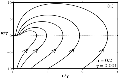
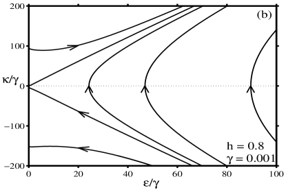
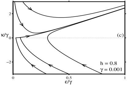
Figure 1: Vector field (22). (a) $A^{2}<\frac{4}{3}$ (here $A^{2}=1.2$); (b) $A^{2}>\frac{4}{3}$ (here $A^{2}=1.8$). (c) gives a blow-up of a small neighbourhood of the origin in (b).

Since the above criterion has been derived under the assumption that $A^{2}$ is not very close to $\frac{4}{3}$, the value $A^{2}=\frac{4}{3}$ provides only a rough watershed between the two types of interaction. In order to establish a more accurate borderline, we zoom in on a narrow strip along the line $A^{2}=\frac{4}{3}$ on the $(\gamma,A^{2})$-plane. Assuming that $|A^{2}-\frac{4}{3}|$ is small (while $\gamma$ is not), Eq.(17a) should be replaced by

$$\pi\dot{\epsilon}=12\left(A^{2}-\frac{4}{3}\right)\kappa\epsilon+\frac{64}{9}\kappa^{3}\epsilon-\frac{64}{3}\kappa\epsilon^{2}.$$ (19)

Substituting (18) into (19) and dropping an ${\cal O}(\epsilon^{7})$ term, we obtain a one-dimensional dynamical system

$$\pi{\dot{\epsilon}}=\frac{256}{\pi\gamma}\left(A^{2}-\frac{4}{3}-\frac{16}{9}\epsilon\right)\epsilon^{3}.$$ (20)

When $A^{2}<\frac{4}{3}$, $\epsilon(t)$ tends to zero for all $\epsilon(0)$. For $A^{2}>\frac{4}{3}$, the system (20) has a stable fixed point at

$$\epsilon=\frac{9}{16}\left(A^{2}-\frac{4}{3}\right).$$ (21)

This fixed point corresponds to a stable bound state of two Néel walls.

When $A^{2}$ approaches $\frac{4}{3}$, the distance $2z=-\ln\epsilon$ between the walls in this bound state tends to infinity and so the bound state does not exist for $A^{2}$ smaller than $\frac{4}{3}$. This means that $A^{2}=\frac{4}{3}$ is, in fact, an accurate borderline between the two types of behaviour. For $A^{2}<\frac{4}{3}$, two walls repel whereas for $A^{2}>\frac{4}{3}$, the walls attract — except for $A^{2}$ close to $\frac{4}{3}$, in which case they form a stable bound state.

We should emphasise here that our present conclusions pertain only to distant walls. In order to extend our understanding of the Néel wall dynamics beyond the limit of very small $\epsilon$, one has to analyse the dynamical system (16) without neglecting any powers of $\epsilon$ and $\kappa$ in it. This will be done numerically in section IV.4 below. We will show, in particular, that in addition to the stable bound state of two walls, there is also an unstable complex — at a shorter distance.

IV.2 $|A^{2}-\frac{4}{3}|={\cal O}(1)$; small $\gamma$

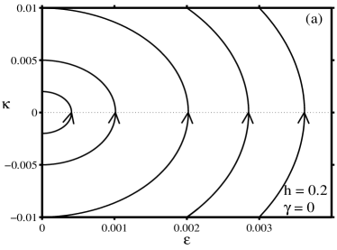
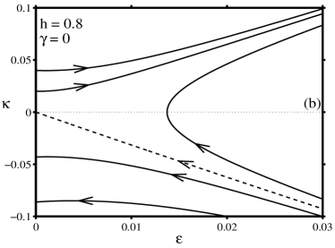
Figure 2: Vector field (22) with $\gamma=0$. (a) $A^{2}<\frac{4}{3}$; (b) $A^{2}>\frac{4}{3}$.

When $\gamma$ is small, the system (16) becomes

$$\pi{\dot{\epsilon}}=12\left(A^{2}-\frac{4}{3}\right)\kappa\epsilon,$$ (22a)

$$\pi({\dot{\kappa}}+2\gamma\kappa)=32A^{2}\epsilon^{2}-24\left(A^{2}-\frac{4}{3}\right)\kappa^{2}\epsilon z.$$ (22b)

For either sign of $A^{2}-\frac{4}{3}$, the origin is the only fixed point in the system. Noting that the $\kappa$-axis ($\epsilon=0$) is an invariant manifold flowing into the fixed point and calculating the index of the vector field (22) along the semicircle $\epsilon^{2}+\kappa^{2}=R^{2}$, $\epsilon\geq 0$, with $R<1$, we conclude that the fixed point is a stable node for $A^{2}<\frac{4}{3}$ and a saddle for $A^{2}>\frac{4}{3}$. Hence, for $A^{2}<\frac{4}{3}$, all trajectories tend to the origin as $t\to\infty$ [Fig.1(a)], i.e., the walls repel.

For $A^{2}>\frac{4}{3}$, all trajectories fly away to infinity [Fig.1(b)] implying the attraction of the walls. One may wonder whether some trajectories coming from the lower half of the phase plane, could flow into the origin (tangent to the vertical axis.) A simple analysis of trajectories in a small neighbourhood of the origin shows that such behaviour is, in fact, impossible. Trajectories which seem to be approaching the point $\epsilon=\kappa=0$ close to the $\kappa$-axis, do turn away when they are a small distance away from the origin. This is illustrated by Fig.1(c) which gives a blow-up of a small neighbourhood of the fixed point.

In the next subsection, we will zoom in on a small neighbourhood of $A^{2}=\frac{4}{3}$ to draw a sharper boundary between domains of the opposite types of interaction — similar to the way we have done it for large $\gamma$. We should also mention here that, as in the previous subsection, our current conclusions pertain to walls with large separations.

The undamped case, $\gamma=0$, is exceptional; in this case, the entire $\kappa$-axis is a line of fixed points — they represent pairs of infinitely separated walls moving at constant velocities. For $A^{2}<\frac{4}{3}$, the points with $\kappa>0$ are stable and those with $\kappa<0$ unstable. Trajectories have the form of arcs starting on the lower semiaxis and flowing into points on the upper semiaxis: $\epsilon(t)\to 0$, $\kappa(t)\rightarrow\kappa_{*}>0$ as $t\rightarrow\infty$ [Fig.2(a)]. The separation between the walls corresponding to the points on the upper semiaxis grows linearly: $z\rightarrow-\frac{6}{\pi}\left(A^{2}-\frac{4}{3}\right)\kappa_{*}t$; that is, the evolution produces two Néel walls moving away from each other at a constant speed.

In the undamped case with $A^{2}>\frac{4}{3}$, the stable points are those with $\kappa<0$ and unstable those with $\kappa>0$. Since ${\dot{\kappa}}>0$ on the horizontal axis (where $\kappa=0$), trajectories starting on the upper semiaxis cannot cross to the negative-$\kappa$ half-plane and have to escape to the positive-$\kappa$ infinity: $\kappa\to\infty$, $\epsilon\to\infty$ as $t\to+\infty$. The same is true for trajectories that have arrived from the negative-$\kappa$ half-plane. Invoking the reversibility of the system (22) with $\gamma=0$, i.e. making use of the invariance under $t\to-t$, $\kappa\to-\kappa$, completes the phase portrait [Fig.2(b)].

To interpret the portrait, we note that $\kappa$ is proportional to ${\dot{z}}$, the velocity of the wall [see Eq.(22a)]. According to Fig.2(b), two walls with zero initial velocities [$\kappa(0)=0$] will attract [$\epsilon(t)\rightarrow\infty$ as $t\rightarrow\infty$]. The same applies, naturally, to the walls whose initial velocities are directed towards each other [$\kappa(0)>0$], and to walls with small outward initial velocities [$\kappa(0)<0$]. However, walls with sufficiently large outward initial velocities will diverge [$\epsilon(t)\rightarrow 0$], with the separation growing linearly: $z(t)\rightarrow-\frac{6}{\pi}\left(A^{2}-\frac{4}{3}\right)\kappa_{*}t$ as $t\rightarrow\infty$. (Here $\kappa_{*}<0$.) The dashed line in Fig.2(b) is a separatrix between initial conditions giving rise to the above two scenarios.

Finally, it is worth mentioning that when $\gamma=0$, equations (15) with $\kappa_{1}=\kappa_{2}=\kappa$ and ${\cal B}=1$ form a hamiltonian system (with a nonstandard bracket):

$$\dot{z}=\frac{1}{\pi\tau}\frac{\partial H}{\partial\kappa},\quad\dot{\kappa}=-\frac{1}{\pi\tau}\frac{\partial H}{\partial z},$$ (23)

where

$$\tau(\epsilon,\kappa)=1+2\epsilon(1-14\epsilon+\kappa^{2}+10\epsilon\kappa^{2})>0,$$ (24)

and the Hamiltonian

$$H(\epsilon,\kappa)=(1-3h)\kappa^{2}-\frac{2}{3}A^{2}\kappa^{4}+4\epsilon\kappa^{2}[(1-3h)z+4h]\\ +\frac{8}{3}\epsilon^{2}[3A^{2}+(12-25A^{2})\kappa^{2}+14A^{2}\kappa^{4}-4A^{2}\kappa^{6}]\\ +16\epsilon^{2}z\kappa^{2}(5A^{2}-4-A^{2}\kappa^{2}).$$ (25)

This observation endows $\kappa$ with a simple interpretation of the momentum canonically conjugate to $z$ — in agreement with qualitative arguments in section III.

IV.3 Small $|A^{2}-\frac{4}{3}|$; small $\gamma$

Finally, let us assume that both $|A^{2}-\frac{4}{3}|$ and $\gamma$ are small. Here, equations (16) are to be replaced by

$$\pi\dot{\epsilon}=12\left(A^{2}-\frac{4}{3}\right)\kappa\epsilon+\frac{64}{9}\kappa^{3}\epsilon-\frac{64}{3}\kappa\epsilon^{2},$$ (26a)

$$\pi(\dot{\kappa}+2\gamma\kappa)=\frac{128}{3}\epsilon^{2}+\frac{32}{3}\epsilon\kappa^{2}.$$ (26b)

Note that we have neglected the term proportional to $z=-\frac{1}{2}\ln\epsilon$ in the second line of (16b). When $A^{2}-\frac{4}{3}<0$, this is justifiable as this term is of the same sign as the last term in the right-hand side of (16b) and so it cannot alter the dynamics qulitatively. The validity of this approximation for $A^{2}-\frac{4}{3}>0$ will be established below.

The dynamics is influenced by nontrivial fixed points which arise as intersections of the nullclines of the system (26):

$$\kappa\epsilon\left(12\mu+\frac{64}{9}\kappa^{2}-\frac{64}{3}\epsilon\right)=0,$$ (27a)

$$\frac{128}{3}\epsilon^{2}+\frac{32}{3}\epsilon\kappa^{2}-2\pi\gamma\kappa=0.$$ (27b)

Here we have introduced

$$\mu=A^{2}-\frac{4}{3}.$$ (28)

The nullcline (27b) emanates out of the origin as a parabola: $\kappa\to\frac{64}{3\pi\gamma}\epsilon^{2}$ as $\epsilon\to 0$; turns back and escapes to infinity asymptotic to the positive $\kappa$-axis: $\kappa\to\frac{3\pi\gamma}{16}\epsilon^{-1}$ as $\epsilon\to 0$. Importantly, it has no points in the $\epsilon>0$, $\kappa<0$ quadrant. The nullcline (27a) consists (apart from the vertical and horizontal axes) of a parabola lying on a side: $\epsilon=\frac{3}{4}\mu+\frac{1}{3}\kappa^{2}$. Intersections of these nullclines are easy to determine and visualise, and the stability of the fixed points can be classified by straightfoward index arguments.

When $\mu<0$, there is only one nullcline intersection in the positive-$\epsilon$ halfplane. It is not difficult to check that this fixed point is a saddle. The origin is also a fixed point — a stable node. The portrait is in Fig.3(a). Distant walls [more precisely, walls with initial conditions lying below the stable manifold of the saddle in Fig.3(a)] repel: $\epsilon(t)\to 0$ as $t\to\infty$. On the other hand, nearby walls (more precisely, those above the stable manifold) attract: $\epsilon(t)\to\infty$.

As $\mu$ grows through zero, another fixed point appears from the negative-$\epsilon$ half-plane. An exchange of stabilities occurs at $\mu=0$: the nontrivial point appearing for $\mu>0$ is a stable node whereas the origin becomes a saddle. The nearby walls attract while distant walls form a stable bound state [Fig.3(b)]. As $\mu$ is increased further, the two nontrivial fixed points merge in a saddle-node bifurcation. When $\mu>\mu_{sn}$, the origin persists as the only fixed point in the system (an unstable one). All walls attract [Fig.3(c)].

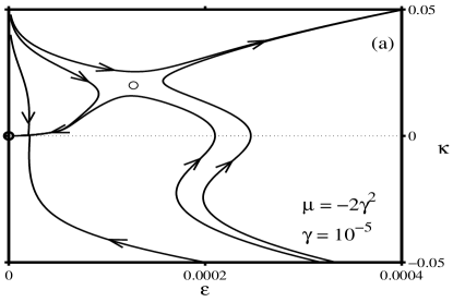
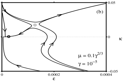
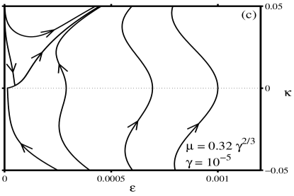
Figure 3: The vector field (26). (a) $\mu<0$ (small initial conditions are attracted to a stable fixed point at the origin; larger initial conditions give rise to trajectories flowing to infinity). (b) $0<\mu<0.3048\gamma^{2/3}$ (initial conditions with small $\epsilon$ and $\kappa$ are attracted to a stable fixed point away from the origin; larger initial conditions give rise to unbounded trajectories). (c) $\mu>0.3048\gamma^{2/3}$ (no stable fixed points, all trajectories flow to infinity). The stable fixed point is marked by a solid blob; the unstable one by an open circle.

Note that the logarithmic term in (16b) that was omitted in (26b), becomes of the same order as the last term in the right-hand side of (16b) only if $z\mu\sim 1$, i.e. when $\epsilon$ is as small as $e^{-2/\mu}$. However, since the nullcline (27a) is bounded from the vertical axis by the inequality $\epsilon\geq\frac{9}{16}\mu$, there can be no fixed points with $\epsilon\sim e^{-2/\mu}$. Therefore the logarithmic term can have no significant effect on the dynamics and its omission is totally legitimate.

To find the threshold $\mu_{sn}(\gamma)$, we eliminate $\kappa$ between (27a) and (27b). The resulting equation can be written as

$$\epsilon\frac{7\epsilon-\frac{27}{16}\mu}{\sqrt{3\epsilon-\frac{27}{16}\mu}}=\frac{3\pi}{16}\gamma.$$ (29)

If $\mu$ is positive, the function $F(\epsilon)$ in the left-hand side of (29) grows to infinity as $\epsilon\to\frac{9}{16}\mu$ and $\epsilon\to\infty$, and has a minimum at $\epsilon=\epsilon_{min}=\frac{1}{126}(31+\sqrt{457})\mu$. The minimum value is $F(\epsilon_{min})=F_{0}\mu^{3/2}$, where $F_{0}$ is a numerical coefficient. Consequently, Eq.(29) has no roots if $\mu>(3\pi/16F_{0})^{2/3}\gamma^{2/3}\approx 0.3048\gamma^{2/3}$ and two roots if $0<\mu<0.3048\gamma^{2/3}$.

According to Eq.(29), when $\gamma$ grows, the “smaller” (stable) fixed point tends to $\epsilon=\frac{9}{16}\mu$; this reproduces Eq.(21) of subsection IV.1.

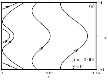
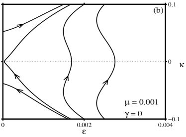
Figure 4: The vector field (26) for $\gamma=0$. (a) $A^{2}<\frac{4}{3}$; (b) $A^{2}>\frac{4}{3}$.

These considerations translate into the following criterion valid for small $\gamma$ and small differences $A^{2}-\frac{4}{3}$. [We are also assuming that the imaginary parts of the perturbation of the walls are small initially, i.e. $\kappa(0)$ is small.] The direction of forces between the walls depends on their position relative to two stationary bound states, a stable (with the interwall separation denoted $2z_{s}$) and an unstable one (with the separation $2z_{u}$). The unstable complex exists for all $A^{2}<A_{sn}^{2}$ while the stable one only for $\frac{4}{3}<A^{2}<A_{sn}^{2}$, where

$$A_{sn}^{2}=\frac{4}{3}+0.3048\gamma^{2/3}.$$ (30)

In their region of coexistence ($\frac{4}{3}<A^{2}<A_{sn}^{2}$), the stable complex has a larger separation: $2z_{s}>2z_{u}$. As $A^{2}\to\frac{4}{3}$, the distance $2z_{s}$ grows to infinity.

When $A^{2}<\frac{4}{3}$, two Néel walls repel if their separation distance is greater than $2z_{u}$. If the initial separation is smaller than $2z_{u}$, the walls attract. It is natural to expect that the attraction should result in the annihilation of the walls, but this diagnosis is beyond the scope of the variational approximation and can only be established in direct numerical simulations of the full partial differential equation (6) (see below).

Next, if $\frac{4}{3}<A^{2}<A_{sn}^{2}$, the walls with separations larger than $2z_{u}$ will move towards the stable equilibrium [from inside or outside depending on whether $z(0)<z_{s}$ or $z(0)>z_{s}$]. The walls at shorter distances, $2z(0)<2z_{u}$, are attracted to each other; they converge and, apparently, annihilate.

Finally, for $A^{2}>A_{sn}^{2}$, the walls are attracted to each other. No complexes, stable or unstable, can be formed for these large $A$.

Like in the large-$|\mu|$ situation, the undamped case ($\gamma=0$) is exceptional in the small-$|\mu|$ region. In this case, the whole $\kappa$-axis is a line of fixed points. When $\mu>0$, the phase portrait [Fig.4(b)] is similar to Fig.2(b). The walls which are initially at rest [$\kappa(0)=0$], attract ($\epsilon\to\infty$ as $t\to\infty$). As for the moving walls with large separations, their initial velocities are determined by $\kappa(0)$:

$${\dot{z}}(0)\approx-\frac{\kappa(0)}{\pi}\left[6\mu+\frac{32}{9}\kappa^{2}(0)\right].$$ (31)

If the walls are initially diverging sufficiently fast, they will continue to do so, with

$$\kappa(t)\to\kappa_{*}<0;\quad z(t)\to-\frac{\kappa_{*}}{\pi}\left(6\mu+\frac{32}{9}\kappa_{*}^{2}\right)t.$$

The portrait for $\mu<0$ is in Fig.4(a). Restricting our analysis to small $|\kappa(0)|$, we observe that walls with large separations repel and small separations attract. This is true both for initially quiescent and slowly moving walls.

IV.4 Numerical study of the fixed points; all $\gamma$

As we have seen in section IV, distant walls with $A^{2}>\frac{4}{3}$ are attracted to each other. Whether the attracting walls are going to form a stable bound state or collide and annihilate, depends on two factors: (i) whether a stable and unstable bound states exist for the corresponding $\gamma$ and $A^{2}$, and if yes, then (ii) how the initial interwall separation compares with $2z_{u}$, the interwall separation in the unstable complex. For small $\gamma$, the region where the two complexes exist was found to be $\frac{4}{3}<A^{2}<A^{2}_{sn}$, with $A^{2}_{sn}$ as in Eq.(30). In order to classify the outcomes of the wall attraction, we need to demarcate the corresponding region for nonsmall $\gamma$ as well.

The one-dimensional dynamical system (20) has only one, stable, fixed point. In order to describe the unstable complex (which is bound tighter than the stable one, i.e. has a greater $\epsilon$), it is sufficient to retain the next, ${\cal O}(\epsilon^{7})$, term in Eq.(19) when we substitute (18) for $\kappa$. However, despite capturing both the stable and unstable bound states, the system (18)-(19) will not produce any reasonably-accurate description of the saddle-node bifurcation where the two fixed points merge and disappear. One reason for this is that the term $32\pi\gamma\epsilon^{2}\kappa^{2}$ in Eq.(16a) which was dropped from Eq.(19), becomes larger than $\epsilon^{7}$ when we substitute (18) for $\kappa$. Another problem is that Eq.(18) keeps only the leading term in the $\kappa(\epsilon)$ expansion; retaining the next, ${\cal O}(\epsilon^{5})$, term in $\kappa(\epsilon)$ produces another term larger than $\epsilon^{7}$ in Eq.(20).

Thus, in order to obtain an accurate variational description of the saddle-node bifurcation, we need to return to the original, nonreduced, vector field (16). Denoting $f(\epsilon,\kappa)$ and $g(\epsilon,\kappa)$ the right-hand sides of (16a) and (16b), the two fixed points arise as intersections of the nullclines

$$f(\epsilon,\kappa)=0,\quad g(\epsilon,\kappa)=0.$$ (32)

The nullclines have a common tangent when

$$\frac{f_{\epsilon}(\epsilon,\kappa)}{f_{\kappa}(\epsilon,\kappa)}=\frac{g_{\epsilon}(\epsilon,\kappa)}{g_{\kappa}(\epsilon,\kappa)}.$$ (33)

Using a standard numerical routine to solve the system (32)-(33) for the vector of unknowns $(\epsilon,\kappa,A^{2})$, one can find the saddle-node value $A_{sn}^{2}$ for each $\gamma$.

The resulting curve $A^{2}=A^{2}_{sn}(\gamma)$ is shown in Fig.7 below (the dotted line), where it is compared to the data from the numerical continuation of the wall complexes as solutions to Eq.(6). The significance of the curve is that it provides a borderline between the two dynamical scenarios: For $A^{2}>A_{sn}^{2}$, two Néel walls attract each other and annihilate; for $\frac{4}{3}<A^{2}<A_{sn}^{2}$, the walls attract and annihilate if the initial separation $2z(0)<2z_{u}$ and form a stable bound state if $2z(0)>2z_{u}$.

Note that the above numerical result is valid both for large and small $\gamma$. For small $\gamma$, our numerical curve $A^{2}_{sn}(\gamma)$ is reproduced by the explicit formula (30).

We conclude this section by mentioning that the unstable fixed point exists for all $A^{2}<\frac{4}{3}$ for which there are Néel walls, i.e. for $1<A^{2}<\frac{4}{3}$. This is a result of the numerical study of the system (32) with $\gamma$ varying from $0$ to $1$ in steps of 0.01, and $A^{2}$ varying from $1$ to $\frac{4}{3}$ in steps of 0.001. The reservation that we should make here, however, is that when $\gamma$ tends to 0 and, simultaneously, $A^{2}$ tends to 1, the coordinate $\kappa$ of the saddle point approaches a value of order 1. This contradicts the assumptions we made in the derivation of the system (16) and so the fixed point in this parameter region cannot represent any bound states of the walls. (The value of the $\kappa$-coordinate is reasonably small only when $\gamma$ is greater than 0.5 or when $|A^{2}-\frac{4}{3}|$ is smaller than 0.01.) Consequently, the variational analysis cannot provide a trustworthy description of the small-distance dynamics of the walls in the $\gamma\approx 0$, $A^{2}\approx 1$ region. The direct numerical simulations of the full NLS equation (6) seem to be the only reliable source of information here.

V Bound state of two dissipative Néel walls

In the previous section we showed that two bound states of Néel walls, a stable and an unstable one, exist in certain parts of the $(\gamma,h)$-plane. Here, we will reobtain these solutions numerically, demarcate their regions of existence and compare these to the corresponding variational results.

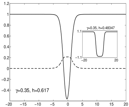
Figure 5: A bubble with a small distance between the walls (a tightly bound complex) looks like a single entity. (Note that the real part does not even reach $-1$ in the core region.) The solid and the dashed lines stand for the real and imaginary part of $\psi$, respectively. For comparison, we also show a bubble with a wide interwall separation arising for $h^{2}$ close to $\gamma^{2}+1/9$ (inset). Here only the real part is shown as ${\rm Im}\,\psi(x)=0$.

We will be using the term “solitonic bubble” as a synonym for the wall complex. Treating bound states as independent soliton-like entities is meant to emphasise the significance of these stationary solutions as possible attractors in the phase space; also, it should reflect their different, nontopological, nature. In fact, when the complex is tightly bound, it looks more like a single entity than a wall doublet; see Fig.5.

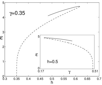
Figure 6: The energy of the dissipative bubble for the fixed $\gamma$ (main panel) and fixed $h$ (inset). The solid and dashed branches indicate stable and unstable solutions, respectively. The stable branch terminates at the point where the distance between the walls becomes infinite; this point is found to coincide with $A^{2}=\frac{4}{3}$. This termination scenario was predicted in section IV using the variational method.

Our approach here is based on the numerical continuation (path-following) of the stationary bubbles as solutions to the ordinary differential equation

$${\textstyle\frac{A^{2}}{2}}\psi_{xx}-A^{2}|\psi|^{2}\psi+\psi+(A^{2}-1)\psi^{*}+i\gamma(\psi-\psi^{*})=0.$$ (34)

The variational approximation (10) with parameters found in subsection IV.3 was used as an initial guess for the numerical solution at small $\gamma$ and $h\approx\frac{1}{3}$; this, in turn, served as a starting point for our continuation. We classified the stability of the resulting stationary complexes as solutions of the full partial differential equation (6), by linearising about the solution and examining the spectrum of the linearised operator numerically.

To present results of the continuation graphically, we use the energy functional

$$E=\frac{1}{2}\int\left\{|\psi_{x}|^{2}+|\psi|^{4}-2\frac{|\psi|^{2}+h\,{\rm Re}(\psi^{2})}{A^{2}}+1\right\}\,dx.$$ (35)

Although the quantity defined in Eq.(35) is not conserved for nonzero $\gamma$, the energy can be used as a bifurcation measure for stationary solutions. [The field momentum (14) is not suitable for this purpose as it satisfies $\dot{P}=-2\gamma P$ and so all stationary solutions with $\gamma\neq 0$ have the same, zero, momentum.]

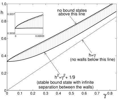
Figure 7: The existence and stability diagram of the bound states on the $(\gamma,h)$-plane (obtained numerically.) The shaded corridor marks the region of coexistence of the stable and unstable bubble. Its upper boundary corresponds to the turning point where the two bubbles merge; there are no bound states above this line. The dotted curve gives the variational approximation (32)-(33) to the line of turning points. The lower boundary of the shaded area corresponds to the stable bound state of two infinitely separated walls (an infinitely long stable bubble). This numerical curve is visually indistinguishable from $h=\sqrt{\gamma^{2}+1/9}$. In the strip between $h=\sqrt{\gamma^{2}+1/9}$ and $h=\gamma$, only the unstable bubble is found. Inset: a blow-up of the small-$\gamma$ region. Here, the dotted curve is plotted using an asymptotic formula (30).

A typical pair of bifurcation diagrams (corresponding to the separate continuations in $h$ and $\gamma$) is presented in Fig.6. [Fig.6 corresponds to $\gamma=0.35$ (main frame) and $h=0.5$ (inset); the continuations for other fixed values of $\gamma$ and $h$ produce curves of similar shape]. Each diagram consists of two branches; the entire branch with higher energy is found to be linearly stable. The solutions on the lower branch are found to be unstable; the instability is associated with a (single) positive real eigenvalue. Numerical simulations of the full time-dependent PDE (6) show that when perturbed, the unstable bubbles decay to the flat solution.

As we approach the termination point of the top branch, the separation of the walls becomes infinite. The termination point satisfies $h\approx\sqrt{\gamma^{2}+1/9}$ (i.e. $A^{2}\approx\frac{4}{3}$) — therefore, this solution reproduces the stable bound state detected by the variational method (sections IV.1, IV.3). The solution on the lower branch corresponds to the unstable complex. We note that this lower branch can be continued all the way to $h=\gamma$, in agreement with variational results in section IV.4.

The walls pull closer together as we move towards the turning point along the upper branch (in the main frame of Fig. 6). As we continue away from the turning point along the bottom branch, the distance between the walls continues to decrease, reaches a minimum, and then starts increasing. This nonmonotonicity can be explained in terms of the fixed points of the dynamical system (26).

The existence and stability of the bound states is summarised in Fig.7. This figure charts the $(\gamma,h)$-plane into regions of different type of interaction between the walls. In the shaded region and above it, distant walls attract each other. The attraction may result in the creation of a stable bound state at some finite separation; this happens in the shaded domain. [The formation of the bound state is illustrated in Fig.8(c) below.] Above the shaded corridor, two attracting Néel walls are expected to collide and annihilate. Finally, in the region between the shaded area and the bisector line $h=\gamma$, two Néel walls at large separation repel.

In Fig.7, we also display the variational results for the saddle-node bifurcation curve $h_{sn}(\gamma)$. The dotted line in the main frame gives the result of solution of the system of three equations (32)-(33) while the dotted line in the inset was plotted using Eq.(30). The variational results are seen to be in good agreement with the outcome of the numerical continuation.

VI Numerical simulations: Néel walls

Conclusions of the variational analysis were verified in direct numerical simulations of the NLS equation (6). We used a split-step pseudospectral method Herbst , with $N=512$ Fourier modes on the interval $(-L/2,\,L/2)=(-40,\,40)$. The numerical scheme is stable for the timesteps $\Delta t<\pi^{-1}(L/N)^{2}$; accordingly, we set $\Delta t=2.5\times 10^{-3}$. The method imposes periodic boundary conditions. The initial condition had the form (10) where $\kappa_{1}$ and $\kappa_{2}$ were set equal to zero. The results are shown in Figs.8, where we have “zoomed in” on the solitons neglecting the flanks of the simulation interval.

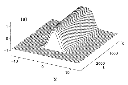
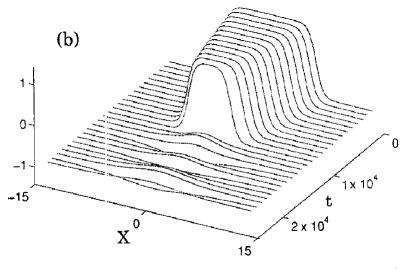
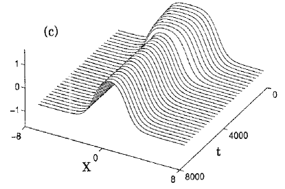
Figure 8: Attraction of two dissipative Néel walls may result either in the annihilation of two walls (a) (here $\gamma=0.1$, $h=0.5$) or formation of a bound state (c) (here $\gamma=0.1$, $h=0.41$). In the absence of damping, the attraction results in the formation of a stationary breather (b) (here $h=0.5$). Simulations reported in panels (a,b) correspond to a point $(\gamma,h)$ lying above the shaded region in Fig.7 while those in panel (c) pertain to a point inside this region. All panels show the real part of $\psi$, multiplied by $-1$ for better visualization.

To verify the diagram of Fig.7, we examined three sequences of points on the $(\gamma,h)$-plane: one just above the shaded region, one just below it, and one inside. The sequence just above the saddle-node line consisted of ten points $\gamma=0.0,0.1,...,0.9$ with $h=0.4+0.75\gamma$. For each pair of parameter values, we examined the initial separations $2z(0)=3.0,4.0$ and $5.0$. The results were in agreement with the diagram of Fig.7: all simulations gave rise to the convergence of the walls. For $\gamma\neq 0$, this resulted in the annihilation of the walls [Fig.8(a)] while in the dissipation-free case, the convergence of the walls ended in the formation of a nonpropagating breather [Fig.8(b)].

The sequence just below the line $h=\sqrt{\gamma^{2}+1/9}$ consisted of $\gamma=0.0,0.1,...,0.9$ with $h=\sqrt{\gamma^{2}+0.09}$. In the $\gamma=0$ case, the walls separated by $2z(0)=4$ were observed to repel whereas those placed at a smaller distance $2z(0)=3$, attracted and formed a nonpropagating breather. These results are in agreement with the variational analysis [see Fig.4(a)]. When $\gamma$ is nonzero, the initial separations $2z(0)=3.0$ and $4.0$ gave rise to the repulsion of the walls. In order to observe the attraction, we had to reduce the initial distance to $2z(0)=1.4$ for $\gamma=0.1$; to $2z(0)=0.8$ for $\gamma=0.2$ and to $2z(0)=0.1$ for $\gamma=0.4$. These observations are consistent with the fact that $z_{u}$, the separation in the unstable complex, becomes smaller as $\gamma$ grows.

Finally, the sequence of points through the dashed region in Fig.7 included $\gamma=0.1,0.2,...,0.8$ with $h=\frac{1}{3}+0.784\gamma$. For these values of $h$, the variational method predicts a tightly bound stable complex of two walls and indeed, in all eight cases the walls with initial separations $2z(0)=3.0,4.0$ and $5.0$ moved towards each other and formed a stable bound state at a certain smaller distance [Fig.8(c)].

Thus the simulations of the Néel wall interactions are in agreement with our expectations for distant-wall dynamics summarised in Fig.7.

VII Two Bloch walls of opposite chiralities

Proceeding to the analysis of Bloch walls, we remind the reader that the Bloch walls exist only for $\gamma=0$ and $h<\frac{1}{3}$; these will be our assumptions in this section. Here, we consider the interaction of two Bloch walls of opposite chiralities (i.e. with total field momentum $P=0$). The corresponding lagrangian arises by setting $\kappa_{1}=\kappa_{2}=\kappa$ and ${\cal B}=B$ in Eq.(13). The resulting equations of motion can be cast in the form of a hamiltonian system

$$\dot{z}=\frac{1}{\pi\tau}\frac{\partial H}{\partial\kappa},\quad\dot{\kappa}=-\frac{1}{\pi\tau}\frac{\partial H}{\partial z},$$ (36)

where $\tau(\epsilon,\kappa)$ is given by Eq.(24), and the Hamiltonian

$$H(\epsilon,\kappa)=-\frac{2A^{2}}{3B}(\kappa^{2}-\kappa_{0}^{2})^{2}+\frac{16h}{B}\epsilon\kappa^{2}\\ +\frac{8}{3B}\epsilon^{2}[7-9h-2(9+5h)\kappa^{2}+(15+11h)\kappa^{4}-4A^{2}\kappa^{6}]\\ +16A^{2}\epsilon^{2}z(2\kappa^{2}-\kappa_{0}^{2}-\kappa^{4}),$$ (37)

with $\epsilon=e^{-2Bz}$ and $\kappa_{0}$ as in (9). Trajectories of the system (36) are simply level curves of the function $H(\epsilon,\kappa)$.

When the interwall separation is large, $\kappa$ should be close to its unperturbed value: $\kappa\approx\kappa_{0}$ or $\kappa\approx-\kappa_{0}$, where $\kappa_{0}$ is, in general, $\mathcal{O}(1)$, but becomes small when $h$ is near $\frac{1}{3}$. In the derivation of the variational equations, we assumed that the walls are well-separated and each wall is close to its unperturbed form. Therefore, only regions around the fixed points ($0,\kappa_{0}$) and ($0,-\kappa_{0}$) can be interpreted within the PDE (6) with full certainty. (Trajectories outside those regions may also have infinite-dimensional counterparts but this requires verification using direct numerical simulations of the full PDE). Note that $\kappa_{0}>0$ is the value of the imaginary part of the right-handed Bloch wall at its center [see Eq.(8)], and $-\kappa_{0}<0$ is the imaginary part of the left-handed Bloch wall at its center. Therefore, the point ($0,\kappa_{0}$) represents a configuration of the right-handed wall at $x=+\infty$ and the left-handed antiwall at $x=-\infty$. The point ($0,-\kappa_{0}$) corresponds to the left-handed wall at $x=+\infty$ and the right-handed antiwall at $x=-\infty$.

Assume, first, that $h$ is not close to $0$ or $\frac{1}{3}$. When $\epsilon$ is small and $\kappa$ is close to $\pm\kappa_{0}$ (which are not small), terms in the third and second lines in (37) are much smaller than the second term in the first line, and can be safely disregarded. The resulting dynamical system

$$\dot{\epsilon}=\frac{16}{3}A^{2}\epsilon\kappa(\kappa^{2}-\kappa_{0}^{2}),\quad\dot{\kappa}=32h\epsilon\kappa^{2},$$

does not have fixed points with nonzero $\epsilon$ and $\kappa$; on the other hand, the entire $\kappa$-axis is a line of nonisolated fixed points. All these points describe pairs of walls moving with constant velocities $\pm{\dot{z}}$, where

$$\dot{z}=-\frac{8(1+h)}{3\pi B}\kappa(\kappa^{2}-\kappa^{2}_{0}).$$

Points on the positive-$\kappa$ semiaxis with $\kappa<\kappa_{0}$ are stable and those with $\kappa>\kappa_{0}$ unstable. Points on the negative-$\kappa$ semiaxis with $\kappa<-\kappa_{0}$ are stable and those with $\kappa>-\kappa_{0}$ unstable. (See Fig.9.) Consequently, walls with large initial separation [$\epsilon(0)$ near $0$] and $\dot{z}(0)>0$ diverge to infinities ($\epsilon\to 0$), whereas distant walls with $\dot{z}(0)\leq 0$ converge.

As for the pairs of walls whose separation is not very large, the situation is straightforward for the walls which are not moving initially [$\dot{z}(0)=0$]; the corresponding initial conditions lie on the straight lines $\kappa=\pm\kappa_{0}$ (dashed lines in Fig.9.) These initial conditions give rise to the convergence of the walls (i.e. $\epsilon$ grows as $t\to\infty$). Otherwise, the type of interaction depends on whether the point $(\epsilon(0),\kappa(0))$ lies to the left or to the right of the heteroclinic trajectory [the trajectory which connects the point $(0,-\kappa_{0})$ to $(0,\kappa_{0})$ — this trajectory is tangent to the vertical axis in Fig.9.]

These variational conclusions are in agreement with direct numerical simulations of the full PDE (6). (We employed the same numerical method as described in section VI.) The initial condition was chosen in the form of two Bloch walls of the opposite chirality which are initially at rest, i.e. Eq.(10) with $\kappa_{1}=\kappa_{2}=\kappa_{0}$. The initially quiescent walls have always been observed to attract; see Fig.10.

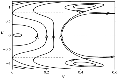
Figure 9: Trajectories of the system (36) obtained as level curves of the Hamiltonian (37). (Here $h=0.1$.) Two points at which the trajectory is tangent to the $\kappa$-axis, correspond to stationary pairs of walls. The dashed lines are $\kappa=\pm\kappa_{0}$; the initial conditions lying on these lines pertain to stationary walls: ${\dot{z}}(0)=0$.

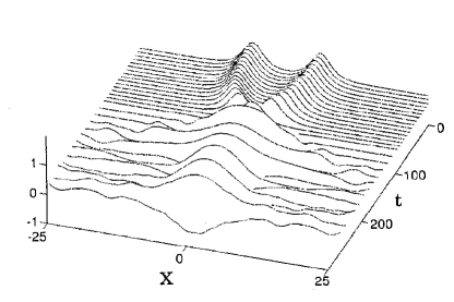
Figure 10: Attraction of Bloch walls with opposite chirality; this attraction results in a long-lived breather. (In this plot, $h=0.1$). To highlight the chiralities of the Bloch walls, the imaginary part of $\psi$ is shown. (We remind that in the case of the wall-antiwall configuration that we are considering, the same signs of the imaginary parts imply opposite chiralities of the walls.)

When $h$ is close to $\frac{1}{3}$, $\kappa_{0}$ is small; since $\kappa$ is assumed to be in the vicinity of $\pm\kappa_{0}$, we cannot neglect terms in the third and second lines in (37) in favour of the first line. However, it is sufficient to keep just the leading term (the term proportional to $7-9h$ in the second line). A straightforward analysis reveals then that the situation here is similar to the one considered above: there are no fixed points with small nonzero $\epsilon$, while the $\kappa$-axis is a line of nonisolated fixed points, stable for $\kappa(\kappa^{2}-\kappa_{0}^{2})<0$ and unstable otherwise. Therefore the phase portrait for small $\epsilon$ and $\kappa$ is similar to the one above.

When $h$ is close to $0$, the last term in the first line of (37) becomes small and hence no terms in the third and second lines can be discarded. In this case, the dynamics can be analysed by plotting level curves of $H$ using standard software. The same approach was adopted to study the vector field outside the small-$\epsilon$ region.

The resulting phase portrait is shown in Fig.9 for $h=0.1$; the portrait does not undergo any qualitative transformations as $h$ is increased up to $\frac{1}{3}$ or decreased down to $0$. A striking feature of Fig.9 is the existence of three families of closed orbits: one centred on a point with $\kappa\approx 1$; a mirror-reflected family centred on a point with $\kappa\approx-1$; and a family of closed trajectories centred on a point on the horizontal axis.

The closed trajectories centered on the fixed point with $\kappa\approx 1$ represent a family of breather solutions of the NLS (1) (and so do their mirror-reflected twins). These breathers have been observed in our numerical simulations of the full partial differential equation (6); see Fig.10. They can also be constructed perturbatively (see section IX below). The nonlinear-center fixed point is sandwiched between two saddles, one below it (clearly visible in Fig.9) and one above. As $h$ is decreased, the two saddle points approach each other. As a result, the periodic orbits are compressed in the vertical direction, and, as $h$ reaches zero, the family of closed trajectories degenerates into a segment of the straight line $\kappa=1$.

The closed loops about a nonlinear-centre fixed point with $\kappa=0$ represent another family of temporally-periodic solutions. Since the value of $\kappa$ for a free-standing wall (i.e. $\kappa_{0}$) is close to zero only when $h$ is close to $\frac{1}{3}$, the family centred on $\kappa=0$ admits a reliable interpretation only in this limit. When $h=0$, the center point has the coordinate $\epsilon\approx 0.06$; as $h$ grows to $\frac{1}{3}$, the centre moves towards the origin so that the family of closed orbits shrinks to a single point $\epsilon=0$, $\kappa=0$. For $h$ close to $\frac{1}{3}$, i.e. in the region where these solutions can be interpreted in terms of the two-wall Ansatz (10), the closed trajectories describe a pair of Bloch walls of opposite chiralities executing periodic oscillations of their separation (but remaining far away from each other.) These oscillatory “doublets” have not yet been observed in direct numerical simulations and their existence remains an open problem. (See the concluding section for a possible explanation of the “nonvisibility” of these objects.)

VIII Two Bloch walls of like chiralities

Finally, we examine the case of a pair of Bloch walls (more precisely, a wall and an antiwall) of the same chirality. As in the previous section, we let $\gamma=0$ and consider $h<\frac{1}{3}$. Assume, for definiteness, that we have a right-handed pair. When at rest, the well-separated wall and antiwall have equal (nonzero) momenta $P_{B}=-\pi\kappa_{0}$ where $\kappa_{0}$ is as in (9). When the walls start moving as a result of their interaction, the total momentum remains the same and hence the individual field momenta of the two walls will change by the same amount: one will become $P_{1}=-\pi(\kappa_{0}+q)$ and the other one $P_{2}=-\pi(\kappa_{0}-q)$. This means that one of the walls will have the amplitude of its imaginary part increase by $q$ and the other one decrease by $q$, and so we will not have a symmetric configuration of an equal-amplitude wall and antiwall any longer. Therefore one may question the validity of our assumption that the two walls remain equal distance away from the origin for $t>0$. To see that the equal-distance Ansatz (10) remains valid — at least for not too late times — we note that the velocity-momentum curve $P(v)$ of a single Bloch wall has a nonzero slope at the point $v=0$, $P=P_{B}$ (see OurPaper ; the curve is also reproduced in part II of the present series of papers BW2 ). This means that the wall whose momentum has increased by $\Delta P=\pi q$, acquires the velocity $\Delta v$, while the wall whose momentum has decreased by $\Delta P=\pi q$, starts moving with the velocity $-\Delta v$ where $\Delta v=(dP/dv)^{-1}\Delta P$. Accordingly, if two walls are equal distance from the origin initially, they will remain equally far from the origin for all $t>0$. This symmetric arrangement will break down only if $\Delta P$ is very large or if $(dP/dv)^{-1}$ is very small, in which case one would have to take into account deviations of the shape of the $P(v)$ curve from a straight line. The derivative $(dP/dv)^{-1}$ tends to zero only if $h\to\frac{1}{3}$ and indeed, numerical simulations do reveal nonsymmetric motion of like-chirality walls when $h$ is very close to $\frac{1}{3}$ (see below), but outside this narrow region the symmetric Ansatz (10) remains valid.

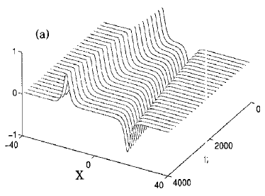
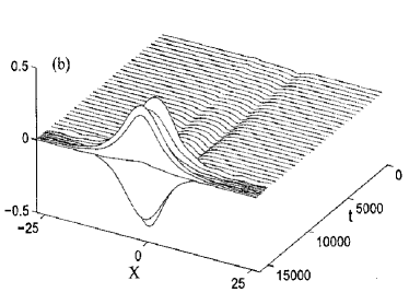
Figure 11: Interaction of Bloch walls of like chiralities. The imaginary part of $\psi$ is shown. (a) Repulsion for generic $h$. (Here $h=0.15$). (b) For $h$ close to $\frac{1}{3}$, the walls may attract and produce a breather on collision. (In this plot, $h=0.333$). Note that before the walls start converging, the wall on the left changes its chirality to the opposite. (We remind that in the case of the wall-antiwall configuration that we are considering, opposite signs of imaginary parts imply like chiralities of the walls.)

Letting $\kappa_{1}=\mp\kappa_{0}+q$, $\kappa_{2}=\pm\kappa_{0}+q$ and ${\cal B}=B$ in the Lagrangian (13), we get equations describing the dynamics of two like-chirality Bloch walls. These can be written as a hamiltonian system

$$\dot{z}=\frac{1}{\pi\tau}\frac{\partial H}{\partial q},\quad\dot{q}=-\frac{1}{\pi\tau}\frac{\partial H}{\partial z},$$ (38a)

where

$$\tau(\epsilon,q)=1+2\epsilon[1-14\epsilon-3(1-6\epsilon)\kappa_{0}^{2}+(1+10\epsilon)q^{2}]>0$$

and the Hamiltonian

$$H(z,q)=-\frac{2A^{2}}{3B}(4\kappa_{0}^{2}+q^{2})q^{2}-\frac{16h}{B}\epsilon(\kappa_{0}^{2}-q^{2})\\ +\frac{8}{3B}\epsilon^{2}\left[7-9h-\frac{\kappa_{0}^{2}}{A^{2}}(7+38h+79h^{2})\right.\\ \left.-\frac{4}{A^{2}}(3+12h+h^{2})q^{2}+(19-h)q^{4}-4A^{2}q^{6}\right]\\ +16\epsilon^{2}z[4h\kappa_{0}^{2}+4(1-h)q^{2}-A^{2}q^{4}].$$ (38b)

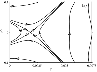
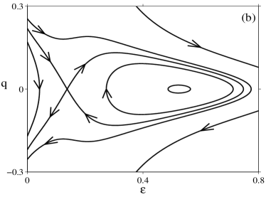
Figure 12: Trajectories of two Bloch walls with like chiralities on the ($\epsilon,q$)-plane. (a) $h$ close to $\frac{1}{3}$ ($h=0.33$ in this plot). Note that the saddle point has small $\epsilon$ here; as a result, there is a region of attraction within the range of validity of the variational approximation. (b) Generic $h$ ($h=0.2$ in this plot). The family of closed orbits describe breather solutions of the NLS (1). Note that unlike in (a), the saddle point and the region of attraction arise at small interwall separations in (b).

Assume, first, that $h$ is not close to $\frac{1}{3}$, so that $\kappa_{0}$ is not a small quantity. In this case the Hamiltonian (38b) with small $\epsilon$ and $q$ is dominated just by two terms,

$$H(z,q)\approx-\frac{8}{3B}A^{2}\kappa_{0}^{2}q^{2}-\frac{16h}{B}\kappa_{0}^{2}\epsilon.$$ (39)

As in the previous section, the $q$-axis in this case is a line of nonisolated fixed points. Since $\dot{z}\approx-(16A^{2}\kappa_{0}^{2}/3\pi B)q$, points with $q>0$ and $q<0$ represent pairs of converging and diverging walls, respectively. The trajectories are parabolas $\epsilon=\epsilon_{*}-(A^{2}/6h)q^{2}$; they start at points on the positive-$q$ semiaxis and flow into points on the negative-$q$ semiaxis. This implies that the initially diverging walls continue to diverge whereas the walls initially moving towards each other shall stop at some finite separation, and then repel to infinities. (A simple but practically important situation concerns walls which are initially at rest; these will obviously start repelling straight away.) The above conclusion applies, of course, only to slowly moving walls which are sufficiently far from each other [i.e. $\epsilon(0)$ and $q(0)$ are small].

Fig.11(a) displays a typical result of direct numerical simulation of the interaction of two like-chirality Bloch walls within Eq.(6). We tested several values of $h$ and a variety of $z(0)$. The initial condition was taken in the form (10) with $\kappa_{1}=-\kappa_{0}$ and $\kappa_{2}=\kappa_{0}$. In agreement with conclusions of the variational analysis, the initially quiescent walls were observed to repel for all $h$ not very close to $\frac{1}{3}$. (The case of $h$ close to $\frac{1}{3}$ is discussed below.)

As $h$ tends to zero, the phase portrait does not undergo any qualitative changes. However, the turning point of the parabola starting at a point $q_{*}$ on the $q$-axis, $\epsilon_{*}=(6h)^{-1/2}Aq_{*}$, is shifted out of the small-$\epsilon$ region, i.e. out of the range of applicability of variational approximation. Consequently, we can no longer expect the initially converging walls to stop a large distance away from each other and repel to infinities after that. Instead, for $h\sim 0$ the colliding like-chirality Bloch walls should penetrate into the core of each other, and the numerical simulations of the full PDE could be the only way to study the outcome of this deep impact.

Next, let $h$ be near $\frac{1}{3}$. In this case the Hamiltonian (38b) with small $\epsilon$ and $q$ reduces to

$$H(z,q)\approx-\frac{8}{9}(4\kappa_{0}^{2}q^{2}+q^{4}+6\kappa_{0}^{2}\epsilon-6\epsilon q^{2}-12\epsilon^{2}).$$

The dynamics with very small $\epsilon$ and $q$ is similar to the one described by Eq.(39): distant pairs of walls with $\dot{z}>0$ diverge while those which are initially set to converge ($\dot{z}<0$) slow down, stop and then repel to infinities [Fig.12(a)]. A new feature in the ($h\approx\frac{1}{3}$)-case is a saddle point at $(\epsilon,q)=(\frac{1}{4}\kappa_{0}^{2},0)$ and a region of attraction which is separated from the region of repulsion by the stable manifold of the saddle [Fig.12(a)]. This fixed point was previously discovered in a variational analysis of the (2:1)-resonantly forced Ginsburg-Landau equation MalNep . Although it would be tempting to think that it represents a stationary complex of two Bloch walls of like chiralities, the actual interpretation of the stationary point turns out to be somewhat different.

Indeed, it was proved in OurPaper2 that in the absence of damping, two Bloch or two Néel walls cannot form stationary complexes. On the other hand, letting $\kappa_{1}=-\kappa_{2}=-\kappa_{0}$ and $e^{-2z}=\kappa_{0}^{2}/4$ with small $\kappa_{0}$, the trial function (10) can be written, approximately, as

$$\mbox{Re}\,\psi=\frac{e^{2x}+e^{-2x}-e^{2z}}{e^{2x}+e^{-2x}+e^{2z}},$$

$$\mbox{Im}\,\psi=\frac{4(e^{x}-e^{-x})}{e^{2x}+e^{-2x}+e^{2z}}.$$

This coincides with the expression for the Bloch-Néel bound state {Eq.(11) of Ref.BW2 } with $s=0$ and $\sigma=-1$, where we only need to send $B\rightarrow 1$ and make the identification $e^{2\beta}=\frac{1}{2}e^{2z}$. Therefore, the “bound state” of two like-chirality Bloch walls produced by the variational analysis is, in fact, the Bloch-Néel complex with $s=0$. The reason why the Bloch-Néel complex could be mistaken for a complex of two Bloch walls, was simply because the Bloch and Néel walls become indistinguishable as $h\to\frac{1}{3}$.

The appearance of the region of attraction for $h$ close to $\frac{1}{3}$ deserves a special comment. The attraction becomes possible due to the smallness of $\kappa_{0}$ in this limit. Indeed, for sufficiently small $\kappa_{0}$, the momentum $\kappa_{1}=\mp\kappa_{0}+q$ becomes close to $\kappa_{2}=\pm\kappa_{0}+q$ — which is characteristic for two Bloch walls of opposite chirality. Thus, in the limit $h\to\frac{1}{3}$, the walls may effectively change their chiralities.

It is instructive to consider the full phase portrait of the system (38); we produce it by plotting level curves of the Hamiltonian (38b) beyond the region of small $\epsilon$ and $\kappa$ [Fig.12(b)]. A remarkable feature here is a family of closed orbits surrounding a nonlinear-center point. The center is born, along with the saddle point, in a saddle-center bifurcation as $h$ is increased past $0.189$. The presence of periodic orbits suggests that breathers may be formed in the collision of Bloch walls of like chirality.

As $h\to\frac{1}{3}$, the saddle point $(\frac{1}{4}\kappa_{0}^{2},0)$ moves closer to the origin and so the periodic orbits pass near $\epsilon=0$. Accordingly, in this limit the breathers should be accessible from initial conditions in the form of well-separated pairs of walls. We note, however, that all closed orbits pass also through a region of large $\epsilon$. [In fact, as $h\to\frac{1}{3}$, the coordinate of the nonlinear center tends to infinity: $\epsilon_{c}\to\exp(1/\kappa_{0}^{2})$.] Consequently, the formation of the breathers requires accurate testing within the full PDE. In our numerical simulations with $h$ close to $\frac{1}{3}$, we have indeed observed the attraction of walls with moderate separations (e.g. with $\epsilon=0.005$ in the case of $h=0.33$ and $\epsilon=0.001$ in the case of $h=0.333$) followed by the formation of a breather [Fig.11(b)]. It is interesting to note that the attraction of two like-chirality walls with $h\sim\frac{1}{3}$ proceeds via the chirality transmutation: first, one of the walls changes its chirality to the opposite; after that, the two opposite-chirality walls attract.

Finally, we need to mention an anomaly in the interaction of two like-chirality walls which was observed in some of our simulations with $h$ near $\frac{1}{3}$. The walls which are initially at rest and equal distance away from the origin, would start moving with different velocities or even in the same direction — violating our Ansatz (10) based on the assumption of a symmetric arrangement for all $t$. This asymmetric anomaly is observed in a wider range of $h$-values near $h=\frac{1}{3}$ than the chirality transmutation (we detected the former for $h$ as far from $\frac{1}{3}$ as $h=0.30$) and has a straightfoward explanation in terms of the $P(v)$ curve. As $h\to\frac{1}{3}$, the derivative $dP/dv$ tends to infinity at the points where the $S$-shaped $P(v)$-curve intersects the $P$-axis and so the equation $\Delta v=(dP/dv)^{-1}\Delta P$ has to be amended by keeping the symmetry-breaking term in $(\Delta P)^{2}$. It is this term that causes the asymmetric motion of the two walls. The anomalous interaction is typical for Bloch-Néel pairs and can be interpreted as the interaction of particles with the opposite mass sign BW2 .

The fact that the motion of two walls has to be asymmetric becomes even more obvious if one notices that the left and right turning points of the $S$-curve approach $v=0$ as $h\to\frac{1}{3}$. As a result, the motion in the direction of the turning point becomes hampered. When $h$ is extremely close to $\frac{1}{3}$, a new channel of interaction becomes available; namely, the wall which is repelled by its partner in the “hard” direction, may “tunnel” through the $P(v)$-barrier by means of the chirality transmutation, and the original symmetric arrangement remains undisturbed.

IX Other localised attractors: nondissipative breathers

In the nondissipative situation ($\gamma=0$), colliding walls form a moving or quiescent breather: a temporally oscillating, spatially localised structure. The breather was formed, for at least a short time, in every undamped collision that we simulated. The formation of the breather is accompanied by the release of a large amount of radiation; the numerical simulations reveal that the breather carries only about a quarter of the energy of the initial configuration, and so the remaining three quarters must escape into the radiation field. As a result, when the interval of simulation is too short, the interaction of the breather with the radiation re-entering the interval via the periodic boundaries is strong enough to destroy it after just a few oscillations. On a large interval, however, the amplitude of the re-entering radiation is small due to the dispersive broadening, and the breather persists indefinitely.

The breather can be easily constructed perturbatively. First of all, a harmonic solution $\delta\psi=e^{i(\omega t-kx)}$ of the NLS (6) linearised about $\psi=1$ obeys the dispersion relation

$$\omega^{2}=\left(1+2h+\frac{k^{2}}{2}\right)^{2}-1.$$

The $(k=0)$-harmonic oscillates with a nonzero frequency $\omega_{0}=2\sqrt{h}A$; therefore, one may also expect to find a broad small-amplitude breather oscillating with that frequency. We write

$$\psi(x,t)=1+\epsilon\psi_{1}(X_{1},X_{2},\dots,T_{0},T_{1},\dots)$$

$$+\epsilon^{2}\psi_{2}(X_{1},X_{2},\dots,T_{0},T_{1},\dots)+\dots,$$ (40)

where $X_{n}=\epsilon^{n}x$, $T_{n}=\epsilon^{n}t$ and $\epsilon$ is a small parameter, and substitute (40) in equation (6). Setting to zero coefficients of $\epsilon^{1}$ and $\epsilon^{2}$, we find:

$$\psi_{1}=u_{1}+iv_{1},\quad\psi_{2}=u_{2}+iv_{2},$$ (41)

where

$$\left(\begin{array}[]{c}u_{1}\\ v_{1}\end{array}\right)=\left(\begin{array}[]{c}2h\\ i\omega_{0}\end{array}\right)\frac{\phi}{2h}e^{i\omega_{0}T_{0}}+c.c.$$ (42)

and

$$\left(\begin{array}[]{c}u_{2}\\ v_{2}\end{array}\right)=\left(\begin{array}[]{c}1+2h\\ i\omega_{0}\end{array}\right)\frac{\phi^{2}}{2h}e^{2i\omega_{0}T_{0}}-\left(\begin{array}[]{c}1+4h\\ 0\end{array}\right)\frac{|\phi|^{2}}{2h}+c.c.$$ (43)

Here the amplitude $\phi$ depends only on long scales $X_{1},X_{2},...$ and slow times $T_{1},T_{2},...$, while $c.c.$ indicates the complex conjugate. The solvability condition at the order $\epsilon^{2}$ is $\partial\phi/\partial T_{1}=0$, so that $\phi$, in fact, is independent of $T_{1}$: $\phi=\phi(X_{1},X_{2},\dots,T_{2},T_{3},\dots)$.

At the order $\epsilon^{3}$, the solvability condition forces $\phi$ to obey the attractive unperturbed nonlinear Schrödinger equation

$$-4i\frac{\sqrt{h}}{A}\frac{\partial\phi}{\partial T_{2}}+(1+2h)\frac{\partial^{2}\phi}{\partial X_{1}^{2}}+8(1+4h)|\phi|^{2}\phi=0.$$ (44)

The breather results if we choose $\phi$ in the form of the soliton:

$$\phi=\phi_{0}\,\mbox{sech}\left[2\sqrt{\frac{1+4h}{1+2h}}\phi_{0}(X_{1}-VT_{2})\right]\quad\quad\quad$$

$$\times\exp\left[-i\frac{A(1+4h)}{\sqrt{h}}\phi_{0}^{2}T_{2}+V\frac{\sqrt{h}}{A(1+2h)}(2X_{1}-VT_{2})\right],$$

(45)

where $\phi_{0}$ and $V$ are free parameters describing the amplitude and velocity of the soliton, respectively. Substituting Eq.(45) into (40)-(42) and defining the amplitude of the breather $a=\epsilon\phi_{0}$ and its velocity $v=\epsilon V$, we obtain, finally,

$$\mbox{Re}\,\psi=1+2a\,\mbox{sech}\left[2\sqrt{\frac{1+4h}{1+2h}}a(x-vt)\right]\cos\left[\Omega t-v\frac{\sqrt{h}}{A(1+2h)}(2x-vt)\right]+\mathcal{O}(\epsilon^{2}),$$ (46a)

$$\mbox{Im}\,\psi=-\frac{2aA}{\sqrt{h}}\mbox{sech}\left[2\sqrt{\frac{1+4h}{1+2h}}a(x-vt)\right]\sin\left[\Omega t-v\frac{\sqrt{h}}{A(1+2h)}(2x-vt)\right]+\mathcal{O}(\epsilon^{2}),\,\,$$ (46b)

where

$$\Omega=\omega_{0}-\frac{A(1+4h)}{\sqrt{h}}a^{2}.$$ (47)

We carried out numerical simulations of Eq.(6) with Eq.(46) as an initial condition, with a variety of (small) values of $a$. (We confined our simulations to the case $v=0$.) For all values of $h$ and $a$ we tried, the breather persisted for the full length of the simulation (approximately $1000$ periods of the breather’s oscillation), with virtually no change. The measured frequency of oscillation coincided with the asymptotic value (47) up to the third decimal place.

Simulations were also performed with a gaussian initial condition

$$\psi=1+\alpha e^{-\beta x^{2}},$$ (48)

for a number of small complex values of $\alpha$ ($|\alpha|\lesssim 0.5$) and positive $\beta$. All runs resulted in the formation of a breather, although in some cases [for $|\alpha|\gtrsim 0.3$], the emerging breather would break into a pair of counterpropagating breathers. In those cases where the emerging breather was nonmoving, its shape and frequency were found to be in an excellent agreement with the asymptotic formula (46).

X Conclusions and Open Problems

In this paper, we studied the interactions between the similar-type dark solitons of the nonlinear Schrödinger equation, i.e. Bloch-Bloch and Néel-Néel interactions. Our approach was based on the variational approximation (also known as the collective-coordinate, or variation-of-action, method). The variational conclusions were verified using numerical continuation of solutions of the stationary damped-driven NLS (34) and via direct numerical simulations of the full partial differential equation (6).

X.1 Conclusions

In the dissipative situation ($\gamma\neq 0$), the only available solitons are the Néel walls. When two Néel walls are very far apart, their interaction is simple: the walls repel if $h^{2}<\gamma^{2}+\frac{1}{9}$ and attract if $h^{2}>\gamma^{2}+\frac{1}{9}$. The repelling walls diverge to infinities; as for the case of attraction, there are two possible scenarios. In order to distinguish between the two, one is led to consider the situation where the walls are closer to each other [but still sufficiently far apart for the large-separation approximation (10) to remain valid.]

At these shorter distances, the dynamics is influenced by two bound states, a stable and an unstable one. The stable bound state exists for $h$ between $\sqrt{\gamma^{2}+1/9}$ and a threshold driving strength $h_{sn}$, and the unstable one exists for all $h<h_{sn}$. Here $h_{sn}^{2}=\gamma^{2}+(A_{sn}^{2}-1)^{2}$ where $A_{sn}^{2}(\gamma)$ is defined as a root of the system (32)-(33). For small $\gamma$, the curve $h_{sn}(\gamma)$ can be described explicitly:

$$h_{sn}=\frac{1}{3}+0.3048\gamma^{2/3}.$$ (49)

[This is Eq.(30) written in terms of $h$ and $\gamma$.] In their region of coexistence, the stable complex has a larger separation: $2z_{s}>2z_{u}$.

When $h$ is smaller than $\sqrt{\gamma^{2}+1/9}$, the walls repel if their separation distance $2z(0)$ is greater than $2z_{u}$, the interwall separation in the unstable complex. If $2z(0)<2z_{u}$, the walls converge and annihilate. (This verdict does not extend to the region where both $h$ and $\gamma$ are small. In this region the variational analysis of the small-separation dynamics is inconclusive.) When $\sqrt{\gamma^{2}+1/9}<h<h_{sn}$, pairs of Néel walls with separations $2z(0)$ larger than $2z_{u}$ evolve towards the stable bound state while those with $2z(0)<2z_{u}$ converge and annihilate. Finally, the walls with $h>h_{sn}$ converge and annihilate irrespectively of their initial separation. These results pertain to walls at shorter distances (which are however sufficiently far apart for the variational approximation to remain valid). In particular, they answer the question as to what finally happens to the two walls attracted from very large distances.

The nondissipative case requires a separate summary. Here the walls can move at constant speeds and the interaction pattern becomes complicated by the presence of inertia. When $h$ is greater than $\frac{1}{3}$ (by small or large value), the Néel walls attract and converge — unless the initial condition corresponds to walls having large and opposite velocities. In the latter case the attraction is unable to stop the diverging walls and they escape to infinities. On the other hand, when $h$ is smaller than $\frac{1}{3}$, the walls repel. The exception here is the case where $h$ is close to $\frac{1}{3}$; in this case walls with very large separations repel whereas walls which are not so far from each other, attract.

In the dissipation-free case, the available dark solitons also include Bloch walls. The interaction between two Bloch walls depends on their relative chiralities: two initially quiescent, oppositely-handed Bloch walls attract while two quiescent walls with like chiralities placed at a large distance away from each other, repel. The exception is the case of $h$ close to $\frac{1}{3}$; in this limit, two walls of like chirality repel at large distances but exhibit anomalous interaction or transmute into an opposite-chirality pair and attract – when placed closer to each other.

These conclusions can be extended to the case of the moving Bloch walls, where one just needs to take their inertia into account. For example, two initially diverging oppositely-handed walls at large separation will continue to diverge despite the attraction whereas two likely-handed walls which were initially moving against each other, will continue to converge (until the repulsion stops them and sends away to infinities).

In addition to the interactions between well-separated walls, we investigated products of their collision. When the system is not damped, the collision of two walls results in a stationary or travelling breather. We reconstructed the numerically found breather as an asymptotic series.

When $\gamma$ is nonzero, oscillations are damped and the only nontrivial product of collision of two Néel walls is a stationary bubble — the bound state of two Néel walls. Using the numerical continuation of solutions to the ODE (34), we demarcated the bubble’s domain of existence in the parameter space. [This domain is, naturally, a subset of the part of the $(\gamma,h)$-plane in which remote walls attract]. The numerical demarcation is in excellent agreement with the domain of existence obtained variationally.

X.2 Open Problems

1. We complete the paper by listing several open problems to which we plan to return in future. One interesting problem that merits further investigation, concerns the (unstable) bubble solution with small $h$ and $\gamma$. (This solution is exemplified by Fig.13.) Our numerics and the variational analysis in section IV.4 show that this solution cannot be regarded as a complex of two Néel walls, not even strongly overlapping ones. Its asymptotic behaviour is closer to that of a Bloch wall; however, Bloch walls do not exist in presence of damping. Furthermore, the bubble cannot be continued to $\gamma=0$ and hence does not have a nondissipative analogue in the form of a bound state of two Bloch, or a Bloch and a Néel, walls. (This follows from the fact that the Néel wall is the only solution in the $\gamma=0$ domain which admits continuation to nonzero $\gamma$ as it is the only solution with zero momentum OurPaper .) Thus a question arises whether the bubble with small $h$ and $\gamma$ could be interpreted as a complex of two hypothetical “dissipative Bloch walls” of opposite chiralities — which do not exist individually but can exist as a bound state due to the cancellation of their opposite momenta. A similar momentum cancellation occurs in the attractive damped-driven NLS where it allows complexes to travel with nonzero speeds despite the fact that their constituent solitons are immobile SIAM .

A related question concerns the short-distance Néel wall dynamics with small $h$ and $\gamma$. This problem is inaccessible to the variational method, and the direct numerical simulations of the full PDE seems to be the only appropriate line of attack here.

2. With regard to the Bloch walls, an open problem concerns the family of closed orbits centred on $\kappa=0$ in Fig.9. When $h$ is close to $\frac{1}{3}$, these periodic orbits can be interpreted within the full partial differential equation (1), as pairs of opposite-chirality Bloch walls executing periodic oscillations of their separation. It is not impossible that these periodic solutions exist also for $h$ not so close to $\frac{1}{3}$ [where the validity of the well-separated Ansatz (10) becomes questionable.] It remains to be understood why these orbits have not been observed in our numerical simulations of Eq.(1), with either $h$. One possible explanation stems from the fact that the nonlinear-center fixed point enclosed by this family of closed orbits, corresponds to a maximum of the energy (13c). Consequently, the nonlinear modes not captured by our two-dimensional Ansatz (10) — such as radiations — should make the point $(\epsilon,\kappa)$ slide downhill towards orbits with larger radii, until it crosses through the homoclinic trajectory and ends up at $\epsilon=0$. [It is pertinent to note here that the centre points enclosed by the other two families of closed orbits in Fig.9 are minima of the energy (13c); this is consistent with the stability of the corresponding breather solutions observed in numerical simulations in Section VI.]

3. Next, it would be interesting to simulate collisions of the like-chirality Bloch walls with $h\sim 0$. This case is not amenable to the variational analysis due to the large extent (“width”) of the walls.

4. It would also be interesting to gain a deeper theoretical insight into the anomalous interaction of the like-chirality Bloch walls arising for $h$ close to $\frac{1}{3}$. The variational approach remains a proper tool here; one should only generalise the Ansatz (10) by allowing nonsymmetric configurations of the walls:

$$\varphi_{1}(x,t)=\tanh{[{\cal B}(x+z_{1})]}-i\kappa_{1}\mbox{sech}[{\cal B}(x+z_{1})],$$

$$\varphi_{2}(x,t)=\tanh{[{\cal B}(x-z_{2})]}+i\kappa_{2}\mbox{sech}[{\cal B}(x-z_{2})].$$

Here $z_{1},z_{2}$ and $\kappa_{1},\kappa_{2}$ are unrelated pairs of variables.

5. Finally, one more future challenge is the analysis of the interaction of two breathers and their synchronisation to a common frequency.

Figure 13: The tightly bound complex of two Néel walls with small $h$ and $\gamma$. The solid and dashed line depict the real and imaginary part, respectively. Note an enormous spatial extent of the bubble.

- (1) J. Lajzerowicz and J.J. Niez, in Solitons and Condensed Matter Physics, edited by A.R. Bishop and T. Schneider, Springer Series in Solid-State Sciences Vol. 8 (Springer-Verlag, Berlin, 1978).
- (2) J. Lajzerowicz and J.J. Niez, J. de Phys. 40, L165 (1979)
- (3) S. Sarker, S.E. Trullinger and A.R. Bishop, Phys. Lett. A 59 255 (1976)
- (4) C. Montonen, Nucl. Phys. B 112, 349 (1976)
- (5) I.V. Barashenkov, S.R. Woodford, E.V. Zemlyanaya, Phys. Rev. Lett. 90, 054103 (2003)
- (6) C. Elphick and E. Meron, Phys. Rev. A 40, 3226 (1989)
- (7) B. Denardo, W. Wright, S. Putterman, and A. Larraza, Phys. Rev. Lett. 64, 1518 (1990)
- (8) W. Chen, L. Lu, and Y. Zhu, Phys. Rev. E 71, 036622 (2005)
- (9) B. Denardo, B. Galvin, A. Greenfield, A. Larraza, S. Putterman and W. Wright, Phys. Rev. Lett. 68, 1730 (1992); G. Huang, S.-Y. Lou, and M. Velarde, Int. J. Bif. Chaos 6, 1775 (1996)
- (10) S. Trillo, M. Haelterman and A. Sheppard, Opt. Lett. 22, 970 (1997)
- (11) L.N. Bulaevskii and V.L. Ginzburg, Sov. Phys. JETP, 18, 530 (1964)
- (12) P. Coullet, J. Lega, B. Houchmanzadeh and J. Lajzerowicz, Phys. Rev. Lett. 65, 1352 (1990); P. Coullet, J. Lega and Y. Pomeau, Europhys. Lett. 15, 221 (1991); D.V. Skryabin, A. Yulin, D. Michaelis, W.J. Firth, G.-L. Oppo, U. Peschel, and F. Lederer, Phys. Rev. E 64, 056618 (2001)
- (13) R. Rajaraman, Phys. Rev. D 15, 2866 (1977); V.I. Karpman and V.V. Solov’ev, Physica D 3, 487 (1981); V.S. Gerdjikov and I.M. Uzunov, Physica D 152-153, 355 (2001)
- (14) K. Kawasaki and T. Ohta, Physica A 116, 573 (1982)
- (15) V.E. Zakharov and A.B. Shabat, Sov. Phys. JETP 37, 823 (1973)
- (16) Y.S. Kivshar and B. Luther-Davies, Phys. Rep. 298, 81 (1998)
- (17) L. Korzinov, M.I. Rabinovich and L.S. Tsimring, Phys. Rev. A 46, 7601 (1992)
- (18) H. Tutu and H. Fujisaka, Phys. Rev. B 50, 9274 (1994)
- (19) I.V. Barashenkov and S.R. Woodford, Interactions of Parametrically Driven Dark Solitons II: Néel-Bloch interactions, nlin.PS/0701005
- (20) R. Rajaraman and E.J. Weinberg, Phys. Rev. D 11, 2950 (1975)
- (21) I.V. Barashenkov and S.R. Woodford, Phys. Rev. E 71, 026613 (2005)
- (22) I.V. Barashenkov and V.G. Makhankov, Phys. Lett. A128, 52 (1988); I.V. Barashenkov and E.Yu. Panova, Physica D 69, 114 (1993)
- (23) B.A. Malomed, Prog. Opt. 43, 71 (2002)
- (24) J.R. Yan and Y.P. Mei, Europhys. Lett. 23, 335 (1993)
- (25) I.V. Barashenkov and E.V. Zemlyanaya, Phys. Rev. Lett. 83, 2568 (1999)
- (26) J.A.C. Weideman and B.M. Herbst, SIAM J. Numer. Anal. 23, 485, (1986)
- (27) B.A. Malomed, A.A. Nepomnyashchy, Europhys. Lett. 27, 649 (1994)
- (28) I.V. Barashenkov and E.V. Zemlyanaya. SIAM J. Applied Maths. 64, 800, (2004)