Optimization of synchronization in gradient clustered networks

Abstract

We consider complex clustered networks with a gradient structure, where sizes of the clusters are distributed unevenly. Such networks describe more closely actual networks in biophysical systems and in technological applications than previous models. Theoretical analysis predicts that the network synchronizability can be optimized by the strength of the gradient field but only when the gradient field points from large to small clusters. A remarkable finding is that, if the gradient field is sufficiently strong, synchronizability of the network is mainly determined by the properties of the subnetworks in the two largest clusters. These results are verified by numerical eigenvalue analysis and by direct simulation of synchronization dynamics on coupled-oscillator networks.

It has been recognized in biological physics that at the cellular level, information vital to the functioning of the cell is often processed on various networks with complex topologies Cell_CM_Overview . At a systems level, organizing information using the network idea has also become fundamental to understanding various biological functions. A key organizational feature in many biological systems is the clustered structure where biophysical and biochemical interactions occur at a hierarchy of levels. Examples include various protein-protein interaction networks Ho:2002 ; SM:2003 and metabolic networks RSMOB:2002 . In biology and network science, a fundamental issue is synchronization Strogatz:2003 ; Network_Synchronization . The aim of this paper is to study synchronization in clustered complex networks with uneven cluster-size distribution and asymmetrical coupling. Since this type of network structure is also important to physical and technological systems such as electronic-circuit networks and computer networks Milo:2002 ; VPV:2002 ; ESMS:2003 , understanding synchronization in such networks will be of broad interest.

There has been recent effort to study synchronization in complex clustered networks PLGK:2006 ; ADP:2006 . A general assumption in these works is that all clusters in a network are on the equal footing in the sense that their sizes are identical and the interactions between any pair of clusters are symmetrical. In realistic applications the distribution of the cluster size can be highly uneven. For example, in a clustered network with a hierarchical structure, the size of a cluster can in general depend on the particular hierarchy to which it belong. More importantly, the interactions between clusters in different hierarchies can be highly asymmetrical. For instance, the coupling from a cluster at a top hierarchy to a cluster in a lower hierarchy can be much stronger than the other way around. An asymmetrically interacting network can in general be regarded as the superposition of a symmetrically coupled network and a directed network, both being weighted. A weighted, directed network is a gradient network TB:2004 ; PLZY:2005 , a class of networks for which the interactions or couplings among nodes are governed by a gradient field. Our interest is then the synchronizability and the actual synchronous dynamics on complex clustered networks with a gradient structure.

For a complex gradient clustered network, a key parameter is the strength of the gradient field between the clusters, denoted by $g$. A central issue is how the network synchronizability depends on $g$. As $g$ is increased, the interactions among various clusters in the network become more directed. From a dynamical-system point of view, uni-directionally coupled systems often possess strong synchronizability NM:2006 ; WLL:2007 . Thus, intuitively, we expect to observe enhancement of the network synchronizability with the increase of $g$. The question is whether there exists an optimal value of $g$ for which the network synchronizability can be maximized. This is in fact the problem of optimizing synchronization in clustered gradient networks, and our findings suggest an affirmative answer to the question. In particular, we are able to obtain solid analytic insights into a key quantity that determines the network synchronizability. The theoretical formulas are verified by both numerical eigenvalue analysis and direct simulation of oscillatory dynamics on the network. The existence of an optimal state for gradient clustered networks to achieve synchronization may have broad implications for evolution of biological networks and for practical applications such as the design of efficient computer networks.

Our general setting is network with $N$ nodes and $M$ clusters, where $n_{m}$ is the size of cluster $m$ and $V_{m}$ denotes the set of nodes it contains ($m=1,...,M$). Each pair of nodes is connected with probability $p_{s}$ in the same cluster and with probability $p_{l}$ in different clusters, where $p_{s}>p_{l}$ PLGK:2006 . For a coupled oscillator network with arbitrary connecting topology, its synchronizability is determined BP:2002 by the interplay between the transverse stability of the local-node dynamics $\mathbf{F}(\mathbf{x})$ and the eigenvalue spectrum of the coupling matrix $C$, which can be sorted conveniently as $\lambda_{1}=0<\lambda_{2}\leqslant\cdots\leqslant\lambda_{N}$, where $\lambda_{1}=0$ underlies the synchronization solution. A typical nonlinear oscillator in the synchronization manifold is transversely stable only when some generalized coupling parameter $\sigma$ falls in a finite range: $\sigma\in[\sigma_{1},\sigma_{2}]$, which is determined by the single-oscillator dynamics. The network is synchronizable if all the normalized eigenvalues except $\lambda_{1}$ can be contained within this range: $\sigma_{1}<\varepsilon\lambda_{2}\leqslant\cdots\leqslant\varepsilon\lambda_{N}<\sigma_{2}$, where $\varepsilon$ is a specific coupling parameter. For convenience, we consider the following class of coupled-map networks: $\mathbf{x}_{t+1}^{i}=\mathbf{f}(\mathbf{x}_{t}^{i})-\varepsilon\sum_{j}C_{ij}\mathbf{H}\left[\mathbf{f}(\mathbf{x}_{t}^{j})\right]$, where $\mathbf{x}_{t+1}^{i}=\mathbf{f}(\mathbf{x}_{t}^{i})$ is a $d$-dimensional map representing the local dynamics of node $i$, $\varepsilon$ is a global coupling parameter, and $\mathbf{H}$ is a coupling function. The rows of the coupling matrix $C$ have zero sum to guarantee an exact synchronized solution: $\mathbf{x}_{t}^{1}=\mathbf{x}_{t}^{2}=...=\mathbf{x}_{t}^{N}=\mathbf{s}_{t}$. For certain types of oscillator dynamics and coupling functions, say, for example, the linearly coupled logistic oscillators we are going to study in the following, $\sigma_{N}$ is sufficiently large HYL:1998 . In such cases the condition $\varepsilon\lambda_{N}<\sigma_{2}$ is naturally satisfied and the synchronizability of network is only determined by $\lambda_{2}$. For simplicity, we will restrict our study to such types of oscillator dynamics and coupling functions.

We first develop a theory for networks consisting of two clusters (the theory can be generalized to multiple-cluster networks). Without a gradient field, the adjacent matrix $A$ is such that $A_{ij}=1$ if there is a link between node $i$ and node $j$, and $A_{ij}=0$ otherwise. To introduce a coupling gradient field from cluster $1$ to cluster $2$, for each inter-cluster link ($i,j$), $i\in V_{1}$ and $j\in V_{2}$, we deduce an amount $g$ from $A_{ij}$ (corresponding to the coupling from node $j$ to node $i$) and add it to $A_{ji}$ so that the total coupling strength is conserved. In this sense the gradient field can be said to point from cluster 1 to cluster 2. The coupling matrix $C$ is defined as $C_{ij}=-A_{ij}/k_{i}$, where $k_{i}=\sum_{j=1}^{N}A_{ij}$ is the weighted degree of node $i$, and $C_{ii}=1$.

The eigenvalue spectra of $C$ and of its transpose $C^{T}$ are identical. Let $\hat{e}_{2}=(e_{1},e_{2},...,e_{n_{1}},e_{n_{1}+1},...,e_{N})^{T}$ be the normalized eigenvector associated with $\lambda_{2}$ of $C^{T}$. Since $\sum_{j=1}^{N}C^{T}_{j,i}=\sum_{j=1}^{N}C_{ij}=0$, the eigenvectors associated with non-zero eigenvalues of $C^{T}$ have zero sum: $\sum_{j=1}^{N}\hat{e}_{2,j}=0$ zerosum . From $C^{T}\hat{e}_{2}=\lambda_{2}\hat{e}_{2}$ we have $\lambda_{2}=\hat{e}_{2}^{T}C^{T}\hat{e}_{2}=\sum_{i,j=1}^{N}e_{i}C_{ij}e_{j}$. For a clustered network, the elements in $\hat{e}_{2}$ have a special distribution: $e_{i}\approx E_{1}$ for $i\in V_{1}$ and $e_{j}\approx E_{2}$ for $j\in V_{2}$ PLGK:2006 , where the two constant values $E_{1}$ and $E_{2}$ can be obtained from the normalization condition $\hat{e}_{2}^{T}\hat{e}_{2}=1$ and the zero-sum property. We obtain $E_{1}=-\sqrt{n_{2}/(n_{1}n_{2}+n_{1}^{2})}$ and $E_{2}=\sqrt{n_{1}/(n_{1}n_{2}+n_{2}^{2})}$ (the signs of $E_{1}$ and $E_{2}$ are interchangeable since $E_{1}E_{2}<0$). This can greatly simplify the calculation of $\lambda_{2}$, which now can be written as $\lambda_{2}\approx\sum_{i=1}^{N}e_{i}\{(C_{i1}+C_{i2}+...+C_{in_{1}})E_{1}+(C_{in_{1}+1}+C_{in_{1}+2}+...+C_{iN})E_{2}\}$. The non-zero elements in $C$ can be calculated as follows. For $i\in V_{1}$, $k_{i}\approx n_{1}p_{s}+n_{2}p_{l}(1-g)$, if $j\in V_{1}$, $C_{ij}=-1/k_{i}\equiv g_{11}$, and there are approximately $n_{1}p_{s}$ non-zero elements for each $i$. If $j\in V_{2}$, we have $C_{ij}=-(1-g)/k_{i}\equiv g_{12}$. For $i\in V_{2}$, $k_{i}\approx n_{2}p_{s}+n_{1}p_{l}(1+g)$, if $j\in V_{1}$, $C_{ij}=-(1+g)/k_{i}\equiv g_{21}$ and, if $j\in V_{2}$, $C_{ij}=-1/k_{i}\equiv g_{22}$. Since $C_{ii}=1$, the calculation can be further simplified as $\lambda_{2}\approx\sum_{i=1}^{n_{1}}e_{i}\{E_{1}+g_{11}E_{1}n_{1}p_{s}+g_{12}E_{2}n_{2}p_{l}\}+\sum_{i=n_{1}+1}^{N}e_{i}\{g_{21}E_{1}n_{1}p_{l}+E_{2}+g_{22}E_{2}n_{2}p_{s}\}$. Using $\sum_{i=1}^{n_{1}}e_{i}\approx n_{1}E_{1}$, $\sum_{i=n_{1}+1}^{N}e_{i}\approx n_{2}E_{2}$ and $n_{1}E_{1}^{2}+n_{2}E_{2}^{2}=1$ (the normalization condition), we obtain

$$\lambda_{2}=1+(E_{1}^{2}n_{1}^{2}g_{11}+E_{2}^{2}n_{2}^{2}g_{22})p_{s}+E_{1}E_{2}n_{1}n_{2}p_{l}(g_{12}+g_{21}).$$ (1)

In Eq. (1), the unity comes from the diagonal elements in $C$, it defines the upper limit for $\lambda_{2}$ (this special case is associated with one-way coupled tree-structure networks NM:2006 ; WLL:2007 ). The second term is contributed by the intra-connection of cluster $1$ and cluster $2$. The last term corresponds to the inter-connection between the clusters. The parameter $g$ is contained in these terms via $g_{ij}$. For a given 2-cluster network, the optimal gradient strength $g_{0}$ that maximizes $\lambda_{2}$ can be determined by setting $\partial\lambda_{2}/\partial g=0$, which gives

$$g_{o}=\frac{2n_{1}-N}{Np_{l}}(p_{s}-p_{l}).$$ (2)

(Please note that in deriving $g_{0}$ we actually get two such values: $g_{0}$ and $g_{0}^{{}^{\prime}}=N(p_{s}+p_{l})/[(N-2n_{1})p_{l}]<-1$. Since in our network model $|g|$ is defined within range $[0,1]$, the value $g_{o}^{{}^{\prime}}$ is therefore discarded.)

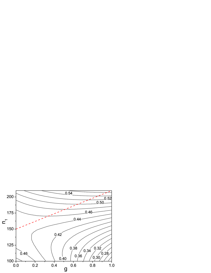
Figure 1: (Color online) Theoretical contour plot of $\lambda_{2}$ in the $(g,n_{1})$ plane, for a $2$-cluster network of $n_{1}+n_{2}=300$ nodes. Other parameters are $p_{l}=0.2$ and $p_{s}=0.7$. The dashed line is given by Eq. (2), which determines, for fixed value of $n_{1}$, the optimal gradient strength $g_{0}$.

Equation (1) reveals some interesting features about the dependence of $\lambda_{2}$ on key parameters of the clustered network. To give an example, we show in Fig. 1 a contour plot of $\lambda_{2}$, calculated using the theoretical formula Eq. (1), in the parameter plane spanned by $n_{1}$ and $g$, where $n_{1}+n_{2}=300$. It gives, for fixed value of $n_{1}$, the dependence of $\lambda_{2}$ on gradient strength. Since, by our construction, the gradient field points from cluster 1 to cluster 2, the upper half region ($n_{1}>150$) in Fig. 1 represents gradient clustered networks for which the gradient field points from the large to the small cluster. For any network defined in this region, for any fixed value of $g$, $\lambda_{2}$ increases monotonically with $n_{1}$, indicating enhanced network synchronizability with the size of the large cluster. However, for a fixed value of $n_{1}$, $\lambda_{2}$ first increases, reaches maximum for some optimal value of $g\equiv g_{0}$, and then decreases with $g$. The dependence of $g_{0}$ on $n_{1}$ is revealed by the dashed line in the figure [Eq. (2)]. We see that, when the gradient field is set to point from the large to the smaller cluster, in order to optimize the network synchronizability, larger gradient strength is needed for larger difference in the cluster sizes. In contrast, in the lower-half of Fig. 1 where $n_{1}<n_{2}$, $\lambda_{2}$ tend to decrease as $g$ is increased (for fixed $n_{1}$) or when the difference between the sizes of the two clusters enlarges. This indicates that, when the gradient points from the smaller to the larger cluster, the network synchronizability continuously weakens as the the gradient field is strengthened.

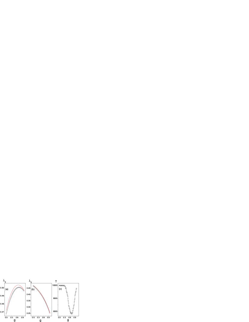
Figure 2: (Color online) For a gradient network of two clusters with $N=300$ nodes, numerically obtained (circles) dependence of $\lambda_{2}$ on the strength $g$ of the gradient field for the two cases where (a) the gradient field points from the larger to the small cluster ($n_{1}=190>N/2$) and (b) the opposite ($n_{1}=110<N/2$). The solid curves are from theory. (c) For $n_{1}=190$, actual synchronization time versus $g$ for a clustered network of chaotic logistic maps. We observe a sharp reduction in the time as $g$ approaches its optimal value, indicating a stronger synchronizability. Other parameters are $p_{l}=0.2$, $p_{s}=0.7$. Each point is the average of 100 random realizations.

To provide support for our theoretical formula Eq. (1), we consider the same network in Fig. 2 and directly calculate the eigenvalue spectrum for a systematically varying set of values of $g$. Figure 2(a) shows $\lambda_{2}$ versus $g$ (open circles) for the case where the gradient field points from the large to the small cluster ($n_{1}=190>N/2$) and Fig. 2(b) is for an opposite case ($n_{1}=110<N/2$). The solid curves are theoretical predictions. We observe a good agreement. To gain insight into the actual dynamics of synchronization on the network, we use the logistic map $f(x)=4x(1-x)$ as the local dynamics, $\varepsilon=1$, and choose $\mathbf{H}(\mathbf{x})=x$ as the coupling function. For the logistic map, we have $\sigma_{1}=0.5$, $\sigma_{2}=1.5$ JJ:2002 . We find numerically $\lambda_{N}\approx 1.1<\sigma_{2}$. Thus the synchronization condition becomes $\lambda_{2}>\sigma_{1}=0.5$. We have calculated the average synchronization time $T$ as a function of $g$, where $T$ is the time needed to reach $\sum_{i=1}^{N}\left|(x^{i}-\langle x\rangle)\right|/N<\delta=10^{-5}$ and $\langle x\rangle\equiv\sum_{i=1}^{N}x^{i}/N$ (the system is considered as unsynchronizable when $T>10^{4}$). As $g$ approaches the optimal value $g_{0}$, we observe a sharp decrease in $T$, as shown in Fig. 2(c), indicating a significant enhancement of the network synchronizability. After reaching the minimum at $g_{0}$, the time increases as $g$ is increased further, as predicted by theory.

The theory we have developed for two-cluster networks can be extended to multiple-cluster networks. Consider a $M$-cluster network, where each cluster contains a random subnetwork. Assume the size of the clusters satisfy $n_{1}>n_{2}>n_{3}\geqslant\cdots\geqslant n_{M}$, a coupling gradient field can be defined as for the two-cluster case. For a random clustered network, the weighted degree can be written as $k_{i}\approx\sum_{j=1}^{N}A_{ij}=n_{m}p_{s}+(N-n_{m})p_{l}+p_{l}g(\sum_{l,n_{m}<n_{l}}n_{l}-\sum_{l^{\prime},n_{m}>n_{l^{\prime}}}n_{l^{\prime}})\equiv K_{m}$. Define $g_{ml}$ as the average value of the non-diagonal, non-zero elements $C_{ij}$. For $i\in V_{m}$ and $j\in V_{l}$, we have $g_{mm}=-1/K_{m}$, $g_{ml}=-(1-g)/K_{m}$ for $n_{m}>n_{l}$, $g_{ml}=-(1+g)/K_{m}$ for $n_{m}<n_{l}$, and $g_{ml}=-1/K_{m}$ for $n_{m}=n_{l}$. For the second eigenvector of $C^{T}$, e.g. $C^{T}\hat{e}_{2}=\lambda_{2}\hat{e}_{2}$, its components have a clustered structure, i.e., for all $i\in V_{m}$, $\hat{e}_{2,i}\approx E_{m}$ while they may vary significantly for different clusters. The eigenvalue $\lambda_{2}$ can then be expressed as $\lambda_{2}=\hat{e}_{2}^{T}C^{T}\hat{e}_{2}=\sum_{i,j=1}^{N}e_{i}C_{ij}e_{j}=\sum_{i=1}^{N}e_{i}\{E_{m}+E_{m}n_{m}p_{s}g_{mm}+\sum_{l\neq m}E_{l}n_{l}p_{l}g_{ml}\}=\sum_{m=1}^{M}n_{m}E_{m}^{2}+\sum_{m=1}^{M}E_{m}^{2}n_{m}^{2}p_{s}g_{mm}+\sum_{l\neq m}E_{m}E_{l}n_{m}n_{l}p_{l}g_{ml}$. Taking into consideration the normalization condition $\hat{e}_{2}^{T}\hat{e}_{2}=1$, we get $\lambda_{2}=1+\sum_{m=1}^{M}E_{m}^{2}n_{m}^{2}p_{s}g_{mm}+\sum_{m,l=1;l\neq m}^{N}E_{m}E_{l}n_{m}n_{l}p_{l}g_{ml}$.

For a general multiple-clustered network, it is mathematically difficult to obtain an analytic formula for the quantity $E_{m}$. However, $E_{m}$ can be determined numerically. Once this is done, the general dependence of $\lambda_{2}$ on $g$ and subsequentially the optimal gradient strength $g_{0}$ can be obtained. In some particular cases, explicit formulas for $E_{m}$ and $\lambda_{2}$ can be obtained. Focusing on the role of the gradient in determining the synchronizability, we consider the extreme gradient case: $g=1$. Numerically, we find that for this case, with respect to the second eigenvector $\hat{e}_{2}$, only $E_{1}$ and $E_{2}$ (corresponding to the largest and the second largest clusters) have non-zero values, while for all $m>2$, $E_{m}=0$. From the normalization condition $\hat{e}_{2}^{T}\hat{e}_{2}=1$ and the zero-sum property $\sum_{j=1}^{N}\hat{e}_{2,j}=0$ (since $\sum_{j=1}^{N}C_{ij}=0$), we can solve for $E_{1}$ and $E_{2}$ as $E_{1}=-\sqrt{n_{2}/(n_{1}n_{2}+n_{1}^{2})}$ and $E_{2}=\sqrt{n_{1}/(n_{1}n_{2}+n_{2}^{2})}$. Noticing $g_{12}=0$, we finally obtain

$$\lambda_{2} = 1+\sum_{m=1}^{2}E_{m}^{2}n_{m}^{2}p_{s}g_{mm}+\sum_{m,l,l\neq m}^{2}E_{m}E_{l}n_{m}n_{l}p_{l}g_{ml}$$ (3)

$$= 1+(E_{1}^{2}n_{1}^{2}g_{11}+E_{2}^{2}n_{2}^{2}g_{22})p_{s}+E_{1}E_{2}n_{1}n_{2}p_{l}g_{21}.$$

A numerical verification of Eq. (3) is provided in Fig. 3(a). An observation is that, except for the difference in $g_{ij}$, Eq. (3) has the same form as Eq. (1), indicating that $\lambda_{2}$ is mainly determined by the first two largest clusters and it has little dependence on the details of size distributions of the remaining clusters. The remarkable implication is that, for different gradient clustered networks, regardless of the detailed form of the cluster size distribution, insofar as the two dominant clusters have similar properties, all networks possess nearly identical synchronizability.

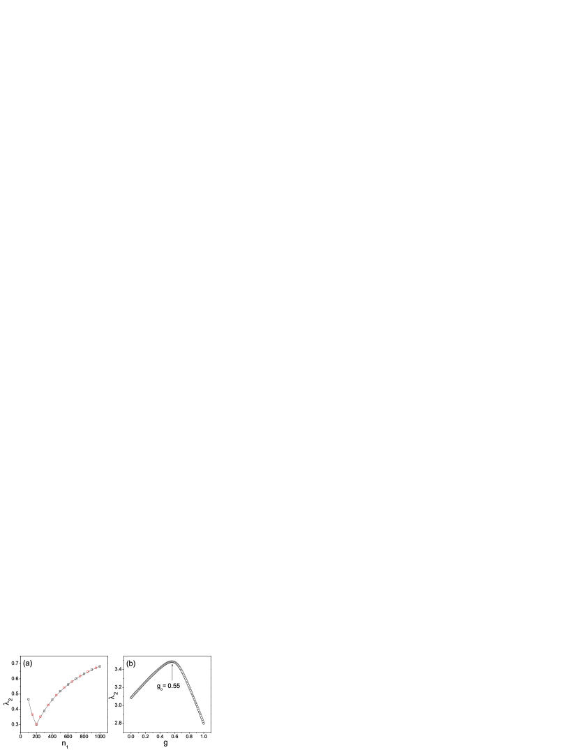
Figure 3: (Color online) (a) For a 5-cluster network (circles) and a 10-cluster network (squares), $\lambda_{2}$ versus $n_{1}$, the size of the largest cluster. The solid curve is from theory [Eq. (3)]. For the 5-cluster network, the size of the remaining clusters are $n_{2}=200$, $n_{3}=50$, $n_{4}=30$, $n_{5}=20$. For the 10-cluster network, we have $n_{2}=200$, $n_{3}$ to $n_{10}$ are $90$, $80$, $70$, $60$, $50$, $40$, $30$, $20$, respectively. Other parameters are $p_{l}=0.15$ and $p_{s}=0.7$. For $n_{1}<n_{2}$, the gradient is actually from cluster 2 to cluster 1. Each point is the average result of $100$ network realizations. (b) For a “cortico-cortical network” of the cat brain, numerical results of the dependence of $\lambda_{2}$ on gradient strength $g$. Synchronization is optimized for $g_{0}\approx 0.55$

The model of gradient clustered network we have investigated here is different to the asymmetrical network models in literature. In Ref. Network_Synchronization ; NM:2006 ; WLL:2007 , asymmetrical couplings have been employed to improve network synchronization and it is found that, for non-clustered networks, synchronization is optimized when all nodes are one-way coupled and the network has a tree-structure NM:2006 . Different to this, in our model asymmetrical couplings are only introduced to inter-cluster links, while couplings on intra-cluster links are still symmetrical. This special coupling scheme induces some new properties to the functions of the gradient. Firstly, increase of gradient will not monotonically enhance synchronization. That is, directed coupling between clusters, i.e. $g=1$, is not always the best choice for synchronization. In many cases the optimal gradient stregth $g_{0}$ is some value between $0$ and $1$, while the exact value is determined by the other network parameters [Eqs. (1,3)]. Secondly, the direction of gradient can not be arranged randomly, it should be always pointing from large to small clusters. Finally, in the case of $g=1$, network synchronizability is still related to the network topology, i.e. by the topology of the first two largest clusters; while for non-clustered network, synchronizability is only determined by the local dynamics NM:2006 .

Can synchronization optimization be expected in realistic networks? To address this question, we have tested the synchronizability of a “cortico-cortical network” of cat brain, which comprises 53 cortex areas and about 830 fiber connections of different axon densities SCANNELL:1999 . The random and small-world properties of this network, as well as its hierarchical structure, have been established in several previous papers CATNET:PROPERTIES . According to their functions, the cortex areas are grouped into 4 divisions of variant size: 16 areas in the visual division, 7 areas in the auditory division, 16 areas in the somato-motor division, and 14 areas in the frontolimbic division. Also, by the order of size, these divisions are hierarchically organized SCANNELL:1999 . With the same gradient strategy as for the theoretical model, we plot in Fig. 3(b) the variation of $\lambda_{2}$ as a function of the gradient strength. Synchronization is optimized at gradient strength about $g_{o}\approx 0.55$. An interesting finding is that the actual average gradient of the real network, $g_{ave}\approx 0.37$ Optimization:real , is deviating from the optimal gradient $g_{o}$, indicating a strong but non-optimized synchronization in healthy cat brain.

While our theory predicts the existence of a gradient field for optimizing the synchronizability of a complex clustered network, we emphasize that the actual value of the optimal gradient field may or may not be achieved for realistic networked systems. Due to the sophisticated procedure involved to determine the optimal gradient strength and the actual value for a given network, their numerical values can contain substantial uncertainties. A reasonable test should involve a large scale comparison across many networks of relatively similar type (say, many different animals), hopefully demonstrating some kind of correlation between the optimum gradient and the observed values. Furthermore, such a test would include a sense of how large the difference between the optimum and observed is. Due to the current unavailability of any reasonable number of realistic complex, gradient, and clustered networks, it is not feasible to conduct a systematic test of our theory. (As a matter of fact, we are able to find only one real-world example of gradient clustered network, the cat-brain network that we have utilized here.) It is our hope that, as network science develops and more realistic network examples are available, our theory and its actual relevance can be tested on a more solid ground.

In summary, we have uncovered a phenomenon in the synchronization of gradient clustered networks with uneven distribution of cluster sizes: the network synchronizability can be enhanced by strengthening the gradient field, but the enhancement can be achieved only when the gradient field points from large to small clusters. We have obtained a full analytic theory for gradient networks with two clusters, and have extended the theory to networks with arbitrary number of clusters in some special but meaningful cases. For a multiple-cluster network, a remarkable phenomenon is that, if the gradient field is sufficiently strong, the network synchronizability is determined by the largest two clusters, regardless of details such as the actual number of clusters in the network. These results can provide insights into biological systems in terms of their organization and dynamics, where complex clustered networks arise at both the cellular and systems levels. Our findings can also be useful for optimizing the performance of technological networks such as large-scale computer networks for parallel processing.

XGW acknowledges the great hospitality of Arizona State University, where part of the work was done during a visit. YCL and LH were supported by NSF under Grant No. ITR-0312131 and by AFOSR under Grant No. FA9550-06-1-0024, and No. FA9550-07-1-0045.

References

- (1) B. P. Kelley, R. Sharan, R. M. Karp, T. Sittler, D. E. Root, B. R. Stockwell, and T. Ideker, Proc. Natl. Acad. Sci. USA 100, 11394 (2003); T. Ideker, Advances in Exp. Med. and Biol. 547, 21 (2004); Y. Xia, H. Yu, R. Jansen, M. Seringhaus, S. Baxter, D. Greenbaum, H. Zhao, and M. Gerstein, Ann. Rev. Biochem. 73, 1051 (2004); M. Lappe, and L. Holm, Nature Biotechnology 22, 98 (2004); A.-L. Barabási and Z. N. Oltvai, Nature Rev. - Genetics 5, 101 (2004).
- (2) Y. Ho, A. Gruhler, A. Heilbut, G. D. Bader, L. Moore, Nature 415, 180 (2002).
- (3) V. Spirin and L. A. Mirny, Proc. Natl. Acad. Sci. (USA) 100, 12123 (2003).
- (4) E. Ravasz, A. L. Somera, D. A. Mongru, Z. Oltvai, and A.-L. Barabási, Science 297, 1551 (2002).
- (5) S. Strogatz, Sync: The Emerging Science of Spontaneous Order (Hyperion, New York, 2003).
- (6) X. F. Wang and G. Chen, Int. J. Bifurcation Chaos Appl. Sci. Eng. 12, 187 (2002); M. Barahona and L. M. Pecora, Phys. Rev. Lett. 89, 054101 (2002); T. Nishikawa, A. E. Motter, Y.-C. Lai, and F. C. Hoppensteadt, Phys. Rev. Lett. 91, 014101 (2003); A. E. Motter, C. S. Zhou, and J. Kurths, Europhys. Lett. 69, 334 (2005); D.-U. Hwang, M. Chavez, A. Amann, and S. Boccaletti, Phys. Rev. Lett. 94, 138701 (2005); C. Zhou and J. Kurths, Chaos 16, 015104 (2006).
- (7) R. Milo, S. Shen-Orr, S. Itzkovitz, N. Kashtan, D. Chklovskii, and U. Alon, Science 298, 824 (2002).
- (8) A. Vázquez, R. Pastor-Satorras, and A. Vespignani, Phys. Rev. E 65, 066130 (2002).
- (9) K. A. Eriksen, I. Simonsen, S. Maslov, and K. Sneppen, Phys. Rev. Lett. 90, 148701 (2003).
- (10) K. Park, Y.-C. Lai, S. Gupte, and J.-W. Kim, Chaos 6, 015105 (2006); L. Huang, K. Park, Y.-C. Lai, L. Yang, and K. Yang, Phys. Rev. Lett. 97, 164101 (2006).
- (11) A. Arenas, A. Díaz-Guilera, and C. J. Pérez-Vicente, Phys. Rev. Lett. 96, 114102 (2006); S. Boccaletti, M. Ivanchenko, V. Latora, A. Pluchino, and A. Rapisarda, Phys. Rev. E 75, 045102 (2007).
- (12) Z. Toroczkai and K.E. Bassler, Nature 428, 716 (2004).
- (13) K. Park, Y.-C. Lai, L. Zhao, and N. Ye, Phys. Rev. E 71, 065105 (2005).
- (14) T. Nishikawa and A. E. Motter, Phys. Rev. E 73, 065106 (2006); ibid, Physica D 224, 77 (2006).
- (15) X.G. Wang, Y.-C. Lai, and C.-H. Lai, Phys. Rev. E 75, 056207 (2006).
- (16) M. B. Barahona and L. M. Pecora, Phys. Rev. Lett. 89, 054101 (2002).
- (17) G. Hu, J. Yang, and W. Liu, Phys. Rev. E 58, 4440 (1998).
- (18) Let , , thus . Therefore . If , then .
- (19) J. Jost and M. P. Joy, Phys. Rev. E 65, 016201 (2002).
- (20) J.W. Scannell et al., Cereb. Cortex 9, 277 (1999)
- (21) C. C. Hilgetag et al., Phil. Trans. R. Soc. B 355, 91 (2000); O. Sporns and J. D. Zwi, Neuroinformatics 2, 145 (2004); C. C. Hilgetag and M. Kaiser, Neuroinformatics 2, 353 (2004); and C. Zhou, L. Zemanova et al., Phys. Rev. Lett. 97 238103 (2006).
- (22) Denoting and the weights of the directed couplings on inter-cluster link , and , and () the size for cluster (). The average gradient of the cat brain network is calculated as , with the number of inter-cluster links.