New approach to the treatment of separatrix chaos
and its application to the global chaos onset between adjacent separatrices

Abstract

We have developed the general method for the description of separatrix chaos, basing on the analysis of the separatrix map dynamics. Matching it with the resonant Hamiltonian analysis, we show that, for a given amplitude of perturbation, the maximum width of the chaotic layer in energy may be much larger than it was assumed before. We apply the above theory to explain the drastic facilitation of global chaos onset in time-periodically perturbed Hamiltonian systems possessing two or more separatrices, previously discovered (PRL 90, 174101 (2003)). The theory well agrees with simulations. We also discuss generalizations and applications. Examples of applications of the facilitation include: the increase of the DC conductivity in spatially periodic structures, the reduction of activation barriers for noise-induced transitions and the related acceleration of spatial diffusion, the facilitation of the stochastic web formation in a wave-driven or kicked oscillator.

I INTRODUCTION

A weak perturbation of a Hamiltonian system causes the onset of chaotic layers around separatrices of the unperturbed system and/or separatrices surrounding nonlinear resonances generated by the perturbation Chirikov:79 ; lichtenberg_lieberman ; Zaslavsky:1991 ; zaslavsky:1998 ; zaslavsky:2005 . The system may be transported along the layer in a random-like fashion and this chaotic transport plays an important role in many physical phenomena Zaslavsky:1991 ; zaslavsky:1998 ; zaslavsky:2005 . If the perturbation is sufficiently weak, then the layers are thin and the chaos is called local Chirikov:79 ; lichtenberg_lieberman ; Zaslavsky:1991 ; zaslavsky:1998 . As the perturbation magnitude increases, the width of the layer grows and the layers corresponding to adjacent separatrices reconnect at some, typically non-small, critical value of the perturbation. This conventionally marks the onset of global chaos Chirikov:79 ; lichtenberg_lieberman ; Zaslavsky:1991 ; zaslavsky:1998 i.e. chaos in a large region of the phase space, with chaotic transport throughout the whole relevant energy range.

The reconnection of the layers around separatrices of the resonances often correlates with the overlap in energy between neighbouring resonances calculated independently in the resonant approximation. The latter constitutes the heuristic Chirikov resonance-overlap criterion Chirikov:79 ; lichtenberg_lieberman ; Zaslavsky:1991 ; zaslavsky:1998 . But the Chirikov criterion may fail if the system is of the zero-dispersion (ZD) type pr i.e. if the frequency of eigenoscillations possesses a local maximum or minimum as a function of its energy (cf. also studies of related maps Howard:84 ; Howard:95 which are called nontwist, twistless or nonmonotonic twist maps). In such systems, there are typically two resonances of one and the same order more , and their overlap in energy does not result in the onset of global chaos pr ; Howard:84 ; Howard:95 . Even their overlap in phase space reconnection results typically only in the reconnection of the thin chaotic layers associated with the resonances. As the amplitude of the time-periodic perturbation grows further, the layers may separate again pr ; Howard:84 ; Howard:95 . An example of the evolution of resonances in the plane of energy and slow angle is given in Fig. 1 (the typical evolution of a real Poincaré section is shown e.g. in comment ).

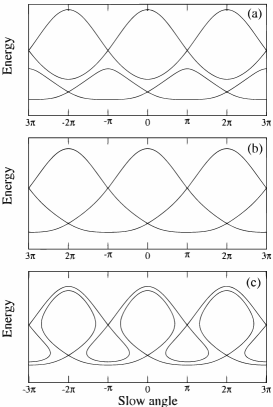
Figure 1: Typical evolution of thin chaotic layers in the plane of slow variables of a zero-dispersion system (the perturbation magnitude grows from the top to the bottom).

As it is known pr , any Hamiltonian system with two or more separatrices belongs to the ZD type: the eigenfrequency as a function of energy possesses a local maximum between each pair of adjacent separatrices. For the purpose of global chaos onset, our letter prl2003 has addressed the possibility to combine the overlap of resonances with each other (typical of ZD systems) and their overlap with the chaotic layers associated with the separatrices. Via numerical simulations, prl2003 demonstrated that this is possible, leading to a scenario for global chaos onset which requires much smaller perturbation amplitudes than in the conventional case. The letter prl2003 suggested also a heuristic theory for this effect (more details were presented in SPIE ).

The present work develops the method for the quantitative description of chaotic layers in phase space, for the resonance frequency range. We uncover the physical mechanism of their overlap with the resonances, and on this basis develop a detailed self-contained theory of the facilitated onset of global chaos. We also discuss generalizations and applications. The method for the description of the chaotic layers is of general importance: in conventional systems with a single-separatrix layer, it predicts a much larger maximum width in energy than what was assumed before Chirikov:79 ; lichtenberg_lieberman ; Zaslavsky:1991 ; zaslavsky:1998 ; zaslavsky:2005 .

The paper is organized as follows. Sec. II introduces some relevant model example and presents the major results of the simulations: studying numerically the frequency dependence of the minimal amplitude of the AC drive for which global chaos occurs, $h_{gc}(\omega_{f})$, we show that $h_{gc}(\omega_{f})$ possesses deep spikes at certain frequencies. Sec. III gives the self-consistent asymptotic theory for the minima of the spikes, after assessing the boundaries of the relevant chaotic layers. Sec. IV gives the theory for the spikes wings. Discussion of a few generalizations and applications is carried out in Sec. V. Conclusions are drawn in Sec. VI. The Appendix describes in details the new method for the analysis of separatrix chaos.

II MODEL AND MAJOR RESULTS OF SIMULATIONS

As an example of a one-dimensional Hamiltonian system possessing two or more separatrices, we use a spatially periodic potential system with two different-height barriers per period (Fig. 2(a)):

$$H_{0}(p,q)=\frac{p^{2}}{2}+U(q),\quad\quad U(q)=\frac{(\Phi-\sin(q))^{2}}{2},$$

$$\Phi={\rm const}<1.$$ (1)

This model may relate e.g. to a pendulum spinning about its vertical axis andronov or to a classical 2D electron gas in a magnetic field spatially periodic in one of the in-plane dimensions oleg98 ; oleg99 . The interest to the latter system arose in the 90th due to technological advances allowing to manufacture magnetic superlattices of high-quality Oleg12 ; Oleg10 leading to a variety of interesting behaviours of the charge carriers in semiconductors oleg98 ; oleg99 ; Oleg12 ; Oleg10 ; Shmidt:93 ; shepelyansky .

Figs. 2(b) and 2(c) show respectively the separatrices of the Hamiltonian system (1) in the $p-q$ plane and the dependence of the frequency $\omega$ of its oscillation, often called eigenfrequency, on its energy $E\equiv H_{0}(p,q)$. The separatrices correspond to energies equal to the value of the potential barrier tops $E_{b}^{(1)}\equiv(1-\Phi)^{2}/2$ and $E_{b}^{(2)}\equiv(1+\Phi)^{2}/2$ (Fig. 2(a)). The function $\omega(E)$ is close to the extreme eigenfrequency $\omega_{m}\equiv\omega(E_{m})$ for most of the range $[E_{b}^{(1)},E_{b}^{(2)}]$ while sharply decreasing to zero as $E$ approaches either $E_{b}^{(1)}$ or $E_{b}^{(2)}$.

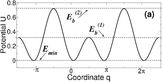
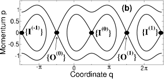
Figure 2: The potential $U(q)$, the separatrices in the phase space and the eigenfrequency $\omega(E)$ for the unperturbed system (1) with $\Phi=0.2$, in (a), (b) and (c) respectively.

Add now a time-periodic perturbation: as an example, we use an AC drive, which corresponds to a dipole Zaslavsky:1991 ; Landau:76 perturbation of the Hamiltonian:

$$\dot{q}=\partial H/\partial p,\quad\quad\dot{p}=-\partial H/\partial q,$$ (2)

$$H(p,q)=H_{0}(p,q)-hq\cos(\omega_{f}t).$$

The conventional scenario of global chaos onset between the separatrices of the system (2)-(1) is illustrated by Fig. 3. The figure presents the evolution of the stroboscopic Poincaré section as $h$ grows while $\omega_{f}$ is fixed at an arbitrarily chosen value away from $\omega_{m}$ and its harmonics. At small $h$, there are two thin chaotic layers around the inner and outer separatrices of the unperturbed system. Unbounded chaotic transport takes place only in the outer chaotic layer i.e. in a narrow energy range. As $h$ grows, so do also the layers. At some critical value $h_{gc}\equiv h_{gc}(\omega_{f})$, the layers merge. This may be considered as the onset of global chaos: the whole range of energies between the barrier levels is involved, with unbounded chaotic transport. The states $\{I^{(l)}\}\equiv\{p=0,q=\pi/2+2\pi l\}$ and $\{O^{(l)}\}\equiv\{p=0,q=-\pi/2+2\pi l\}$ (where $l$ is any integer) in the Poincaré section are associated respectively with the inner and outer saddles of the unperturbed system, and necessarily belong to the inner and outer chaotic layers, respectively. Thus, the necessary and sufficient condition for global chaos onset may be formulated as the possibility for the system placed initially in the state $\{I^{(0)}\}$ to pass beyond the neighbouring of the “outer” states, $\{O^{(0)}\}$ or $\{O^{(1)}\}$, i.e. the coordinate $q$ becomes $<-\pi/2$ or $>3\pi/2$ at sufficiently large times $t\gg 2\pi/\omega_{f}$.

Figure 3: The evolution of the stroboscopic (at $t=n2\pi/\omega_{f}$ with $n=0,1,2,...$) Poincaré section of the system (2)-(1) with $\Phi=0.2$ as $h$ grows while $\omega_{f}=0.3$. The number of points in each trajectory is 2000. In (a) and (b), three characteristic trajectories are shown: the inner trajectory starts from the state $\{I^{(0)}\}\equiv\{p=0,q=\pi/2\}$ and is chaotic but bounded in space; the outer trajectory starts from $\{O^{(0)}\}\equiv\{p=0,q=-\pi/2\}$ and is chaotic and unbounded in coordinate; the third trajectory is an example of a regular trajectory separating the two chaotic ones. In (c), the chaotic trajectories mix.

A diagram in the $h-\omega_{f}$ plane, based on the above criterion, is shown in Fig. 4. The lower boundary of the shaded area represents the function $h_{gc}(\omega_{f})$. It has deep spikes i.e. cusp-like local minima. The most pronounced spikes are situated at frequencies $\omega_{f}=\omega_{s}^{(j)}$ that are slightly less than the odd multiples of $\omega_{m}$,

$$\omega_{s}^{(j)}\approx\omega_{m}(2j-1),\quad\quad j=1,2,...$$ (3)

The deepest minimum occurs at $\omega_{s}^{(1)}\approx\omega_{m}$: the value of $h_{gc}$ in the minimum, $h_{s}^{(1)}\equiv h_{gc}(\omega_{s}^{(1)})$, is approximately 40 times smaller than the value in the neighbouring pronounced local maximum of $h_{gc}(\omega_{f})$ at $\omega_{f}\approx 1$. As $n$ increases, the $n$th minimum becomes less deep. The function $h_{gc}(\omega_{f})$ is very sensitive to $\omega_{f}$ in the vicinity of the minima: for example, a shift of $\omega_{f}$ down from $\omega_{s}^{(1)}\approx 0.4$ by only 1% causes an increase of $h_{gc}$ by $\approx 30\%$.

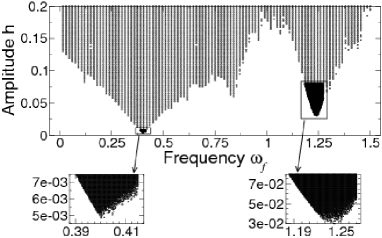
Figure 4: The diagram indicating (shade) the perturbation parameters range for which global chaos exists. Integration time for each point of the grid is $12000\pi$.

The origin of the spikes becomes more clear looking at the evolution of the Poincaré section for $\omega_{f}\approx\omega_{s}^{(1)}$ as $h$ grows (Fig. 5): it drastically differs from the conventional evolution shown in Fig. 3. For $h=0.001$ (Fig. 5(a)), one can see four chaotic trajectories. Two of them are associated with the inner and outer separatrices of the unperturbed system, similarly to the conventional case (cf. Fig. 3). They are marked by green and blue respectively. These trajectories fill the corresponding chaotic layers, which will be referred below as the “inner” and “outer” separatrix layers respectively. The other two chaotic trajectories marked by red and cyan are associated with the two nonlinear resonances of the 1st order. Examples of non-chaotic trajectories separating the chaotic ones are shown in brown. As the perturbation amplitude $h$ increases, the outer separatrix layer sequentially absorbs other chaotic trajectories while large stability islands (associated with the resonances) arise in the layer. At $h=0.003$, it has absorbed the red trajectory: the resulting chaotic layer is shown in blue in Fig. 5(b). At $h=0.00475$, this chaotic layer has absorbed the cyan chaotic trajectory: the resulting chaotic layer is shown in blue in Fig. 5(c) 20_prime . Finally, at $h=0.0055$ the latter blue layer has merged with the inner separatrix layer footnote2 (see Fig. 5(d)), i.e. the onset of global chaos as defined above has occurred.

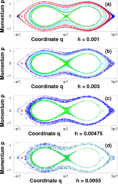
Figure 5: The evolution of the stroboscopic Poincaré section of the system (2)-(1) with $\Phi=0.2$ as the amplitude of the perturbation $h$ grows while the frequency is fixed at $\omega_{f}=0.401$. The number of points in each trajectory is 2000. The chaotic trajectories starting from the states $\{I^{(0)}\}$ and $\{O^{(0)}\}$ are drawn in green and blue respectively. The stable stationary points of Eq. (14) (the 1st-order nonlinear resonances) are indicated by the red and cyan crosses. The chaotic layers associated with the resonances are indicated in red and cyan respectively, unless they merge with those associated with the green/blue chaotic trajectories. Examples of regular trajectories embracing the state $\{I^{(0)}\}$ while separating various chaotic trajectories are shown in brown.

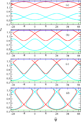
Figure 6: The evolution of the separatrices (full lines) of the 1st-order resonances within the resonance approximation (described by (4) with $n=1$) in the plane of action $I$ and slow angle $\tilde{\psi}$, for the same parameters as in Fig. 5. Horizontal levels mark the values of $I$ corresponding to the barriers.

Even prior to the theoretical analysis, one can draw a few conclusions from the evolution. Namely, if $\omega_{f}$ is close to the minimum of the spike of $h_{gc}(\omega_{f})$, then

• the onset of global chaos occurs due to the combination of the overlap of chaotic layers associated with nonlinear resonances with each other and the overlap of the latter layers with the inner and outer separatrix layers;

• the width of the nonlinear resonances are large already at quite small amplitudes of the perturbation, so that the overlap with the chaotic layers around the original separatrices occurs at unusually small perturbation amplitudes;

• the onset of the overlap of at least one of the nonlinear resonances with the outer separatrix layer occurs at values of $h$ which are a few times smaller than those required for the onset of the overlap with the inner separatrix layer.

The above conclusions are also illustrated by Fig. 6 which presents the evolution of the phase space of slow variables Chirikov:79 ; lichtenberg_lieberman ; Zaslavsky:1991 ; zaslavsky:1998 ; zaslavsky:2005 ; pr , action $I\equiv I(E)$ and slow angle $\tilde{\psi}\equiv\psi-\omega_{f}t$, calculated in resonance approximation for the 1st-order spike (see Eq. (4) below).

Similarly, for the spikes of higher order, higher-order resonances are relevant.

III EXPLICIT ASYMPTOTIC THEORY FOR THE MINIMA OF THE SPIKES

The eigenfrequency $\omega(E)$ is close to its local maximum $\omega_{m}$ for most of the relevant range $[E_{b}^{(1)},E_{b}^{(2)}]$ (Fig. 2(c)). As shown below, $\omega(E)$ approaches a rectangular form in the asymptotic limit $\Phi\rightarrow 0$. Hence, if the perturbation frequency $\omega_{f}$ is close to $\omega_{m}$ or its odd multiples, $|\omega_{f}-(2j-1)\omega_{m}|\ll\omega_{m}$, then the energy width of nonlinear resonances becomes comparable to the width of the whole range between barriers (i.e. $E_{b}^{(2)}-E_{b}^{(1)}\approx 2\Phi$) at a rather small perturbation magnitude $h\ll\Phi$. Note that $\Phi$ determines the characteristic magnitude of the perturbation required for the conventional overlap of the separatrix chaotic layers, when $\omega_{f}$ is not close to any odd multiple of $\omega_{m}$ (Fig. 3 (c)). Thus, if $\omega_{f}\approx\omega_{s}^{(j)}$, the nonlinear resonances should play a crucial role in the onset of global chaos (cf. Fig. 5).

We note that it is not entirely obvious a priori whether it is indeed possible to calculate $h_{s}^{(j)}\equiv h_{gc}(\omega_{s}^{(j)})$ within the resonance approximation: in fact, it is essential for the separatrices of nonlinear resonances to nearly touch the barriers levels, but the resonance approximation is obviously invalid in the close vicinity of the barriers; furthermore, numerical calculations of resonances show that, if $\omega_{f}\approx\omega_{s}^{(j)}$, the perturbation amplitude $h$ at which the resonance separatrix touches a given energy level in the close vicinity of the barriers is very sensitive to $\omega_{f}$, apparently making the calculation of $h_{s}^{(j)}$ within the resonance approximation even less feasible.

Nevertheless, we show below in a self-consistent manner that, in the asymptotic limit $\Phi\rightarrow 0$, the relevant boundaries of the chaotic layers lie in the range of energies $E$ where $\omega(E)\approx\omega_{m}$. Therefore, the resonant approximation is valid and it allows to obtain explicit asymptotic expressions both for $\omega_{s}^{(j)}$ and $h_{s}^{(j)}$, and for the wings of the spikes in the vicinities of $\omega_{s}^{(j)}$.

The asymptotic limit $\Phi\rightarrow 0$ is the most interesting one from a theoretical point of view since this limit leads to the strongest facilitation of the global chaos onset and it is most accurately described by the self-contained theory. Most of the theory presented below assumes this limit and concentrates therefore on the results to the lowest order in the small parameter.

On the applications side, the range of moderately small $\Phi$ is more interesting, since the chaos facilitation is still pronounced (and still described by the asymptotic theory) while the area of chaos between the separatrices is not too small (comparable with the area inside the inner separatrix): cf. Figs. 2, 3 and 5. To increase the accuracy of the theoretical description in this range, we estimate the next-order corrections and develop an efficient numerical procedure allowing for the further corrections.

III.1 Resonant Hamiltonian and related quantities

Let $\omega_{f}$ be close to the $n$th odd even harmonic of $\omega_{m}$, $n\equiv(2j-1)$. Over most of the range $[E_{b}^{(1)},E_{b}^{(2)}]$, except in the close vicinities of $E_{b}^{(1)}$ and $E_{b}^{(2)}$, the $n$th harmonic of eigenoscillation is nearly resonant with the perturbation. Due to this, the (slow) dynamics of the action $I\equiv I(E)=(2\pi)^{-1}\oint dqp$ and the angle $\psi$ Chirikov:79 ; lichtenberg_lieberman ; Zaslavsky:1991 ; zaslavsky:1998 ; zaslavsky:2005 ; pr ; Howard:84 ; Howard:95 ; Landau:76 can be shown to be described by the following auxiliary Hamiltonian (cf. Chirikov:79 ; lichtenberg_lieberman ; Zaslavsky:1991 ; zaslavsky:1998 ; zaslavsky:2005 ; pr ; Howard:84 ; Howard:95 ):

$$\tilde{H}(I,\tilde{\psi})=\int_{I(E_{m})}^{I}{\rm d}\tilde{I}\;(n\omega-\omega_{f})\;-\;nhq_{n}\cos(\tilde{\psi})$$ (4)

$$\quad\;\equiv\;n(E-E_{m})-\omega_{f}(I-I(E_{m}))\;-\;nhq_{n}\cos(\tilde{\psi})\;,$$

$$I\equiv I(E)=\int_{E_{\rm min}}^{E}\frac{{\rm d}\tilde{E}}{\omega(\tilde{E})},\quad\quad E\equiv H_{0}(p,q),$$

$$\tilde{\psi}=n\psi-\omega_{f}t,\quad\quad$$

$$\psi=\pi+{\rm sgn}(p)\omega(E)\int^{q}_{q_{\rm min}(E)}\frac{{\rm d}\tilde{q}}{\sqrt{2(E-U(\tilde{q}))}}+2\pi l,$$

$$q_{n}\equiv q_{n}(E)=\frac{2}{\pi}\int_{0}^{\pi/2}\!\!\!\!\!{\rm d}\psi\;q(E,\psi)\cos(n\psi),$$

$$|n\omega-\omega_{f}|\ll\omega,\quad\quad n\equiv 2j-1,\quad\quad j=1,2,3,\ldots,$$

where $E_{\rm min}$ is the minimal energy (over all $q,p$) $E\equiv H_{0}(p,q)$; $\omega\equiv\omega(E)=dH_{0}/dI$ and $q_{\rm min}(E)$ are, respectively, the frequency and the minimal coordinate of the conservative motion with a given value of energy $E$; $l$ is the number of right turning points in the trajectory $[q(\tau)]$ of the conservative motion with energy $E$ and given initial state $(q_{0},p_{0})$.

Let us derive the explicit expressions for various quantities in (4). In the unperturbed case ($h=0$), the equations of motion (2) with $H_{0}$ (1) can be integrated oleg99 (see also Eq. (60) below), so that we can find $\omega(E)$:

$$\omega(E)=\frac{\pi(2E)^{1/4}}{2K\left[k\right]},$$ (5)

$$k=\frac{1}{2}\sqrt{\frac{(\sqrt{2E}+1)^{2}-\Phi^{2}}{\sqrt{2E}}}\,,$$

where

$$K[k]=\int_{0}^{\frac{\pi}{2}}\frac{{\rm d}\phi}{\sqrt{1-k^{2}\sin^{2}(\phi)}},$$ (6)

is the full elliptic integral of the first order Abramovitz_Stegun . Using its asymptotic expression,

$$K[k\rightarrow 1]\simeq\frac{1}{2}\ln\left({16\over 1-k^{2}}\right),$$

we derive $\omega(E)$ in the asymptotic limit $\Phi\rightarrow 0$:

$$\omega(E)\simeq\frac{\pi}{\ln\left(\frac{64}{(\Phi-\Delta E)(\Phi+\Delta E)}\right)},$$ (7)

$$\Delta E\equiv E-\frac{1}{2},\quad\quad|\Delta E|<\Phi,$$

$$\Phi\rightarrow 0.$$

The function $\omega(E)$ (7) is close to its maximum

$$\omega_{m}\equiv\max_{[E_{b}^{(1)},E_{b}^{(2)}]}\{\omega(E)\}\simeq\frac{\pi}{2\ln(8/\Phi)}\,$$ (8)

for most of the interbarrier barriers range of energies $[1/2-\Phi,1/2+\Phi]$; on the other hand, in the close vicinity of the barriers, where either $|\ln(1/(1-\Delta E/\Phi))|$ or $|\ln(1/(1+\Delta E/\Phi))|$ become comparable with, or larger than, $\ln(8/\Phi)$, $\omega(E)$ sharply decreases to zero as $|\Delta E|\rightarrow\Phi$. The range where this takes place is $\sim\Phi^{2}$, and its ratio to the whole interbarrier range, $2\Phi$, is $\sim\Phi$ i.e. it goes to zero in the asymptotic limit $\Phi\rightarrow 0$: in other words, $\omega(E)$ approaches a rectangular form. As it will be clear from the following, it is this almost rectangular form of $\omega(E)$ which determines many of the characteristic features of the global chaos onset in systems with two or more separatrices.

One more quantity which strongly affects $(\omega_{s},h_{s})$ is the Fourier harmonic $q_{n}\equiv q_{n}(E)$. The system stays most of the time very close to one of the barriers. Consider the motion within one of the periods of the potential $U(q)$, between neighboring upper barriers $[q_{ub}^{(1)},q_{ub}^{(2)}]$ where $q_{ub}^{(2)}\equiv q_{ub}^{(1)}+2\pi$. If the energy $E\equiv 1/2+\Delta E$ lies in the relevant range $[E_{b}^{(1)},E_{b}^{(2)}]$, then the system will stay close to the lower barrier $q_{lb}\equiv q_{ub}^{(1)}+\pi$ for a time arbitrary_constant

$$T_{l}\approx 2\ln\left(\frac{1}{\Phi+\Delta E}\right)$$ (9)

during each period of eigenoscillation, while it will stay close to one of the upper barriers $q_{ub}^{(1,2)}\equiv q_{lb}\pm\pi$ for most of the remaining of the eigenoscillation,

$$T_{u}\approx 2\ln\left(\frac{1}{\Phi-\Delta E}\right)\quad.$$ (10)

Hence, the function $q(E,\psi)-q_{lb}$ may be approximated by the following piecewise even periodic function:

$$q(E,\psi)-q_{lb}=\left\{{}_{0\quad{\rm at}\quad\psi\in\left.\right]\frac{\pi}{2}\frac{T_{u}}{T_{l}+T_{u}},\pi-\frac{\pi}{2}\frac{T_{u}}{T_{l}+T_{u}}\left[\right.,}^{\pi\quad{\rm at}\quad\psi\in\left[0,\frac{\pi}{2}\frac{T_{u}}{T_{l}+T_{u}}\right]\cup\left[\pi-\frac{\pi}{2}\frac{T_{u}}{T_{l}+T_{u}},\pi\right],}\right.$$

$$q(E,-\psi)-q_{lb}=q(E,\psi)-q_{lb},$$

$$q(E,\psi\pm 2\pi i)=q(E,\psi),$$

$$i=1,2,3,...$$

Substituting the above approximation for $q(E,\psi)$ into the definition of $q_{n}$ (4), one can obtain:

$$q_{2j-1}\equiv q_{2j-1}(E)=\frac{2}{2j-1}\sin\left(\frac{(2j-1)\pi/2}{1+\frac{\ln\left(\frac{1}{\Phi+\Delta E}\right)}{\ln\left(\frac{1}{\Phi-\Delta E}\right)}}\right)\;,$$

$$\Phi\rightarrow 0,$$

$$q_{2j}=0,$$ (11)

$$j=1,2,3,...$$

At barrier energies, $q_{2j-1}$ takes the values

$$q_{2j-1}(E_{b}^{(1)})=0,\quad\quad q_{2j-1}(E_{b}^{(2)})=-(-1)^{j}{2\over(2j-1)}\,.$$

As $E$ varies in between the barrier values, $q_{2j-1}$ varies monotonously if $j=1$ and non-monotonously otherwise (cf. Fig. 11). But in any case, the significant variations occur mostly in the close vicinity of the barrier energies $E_{b}^{(1)}$ and $E_{b}^{(2)}$ while, for most of the range $[E_{b}^{(1)},E_{b}^{(2)}]$, the argument of the sine in Eq. (11) is close to $\,\pi/4$ and $\,q_{2j-1}$ is then almost constant:

$$q_{2j-1}\approx(-1)^{\left[\frac{2j-1}{4}\right]}\frac{\sqrt{2}}{2j-1},\quad\ j=1,2,3,\,\ldots,$$ (12)

$$\left|\ln\left(\frac{1+\Delta E/\Phi}{1-\Delta E/\Phi}\right)\right|\ll 2\ln\left(\frac{1}{\Phi}\right),$$

where $[\ldots]$ means the integer part.

In the asymptotic limit $\Phi\rightarrow 0$, the range of $\Delta E$ where the approximate equality (12) for $q_{2j-1}$ is valid approaches the whole range $]-\Phi,\Phi[$.

We emphasize that $|q_{n}|$ determines the “strength” of the nonlinear resonances: therefore, apart from the nearly rectangular form of $\omega(E)$, the non-smallness of $|q_{n}|$ is one more factor giving rise to the strong facilitation of the global chaos onset.

We shall need also the asymptotic expression of the action $I$. Substituting $\omega(E)$ (7) into the definition of $I(E)$ (4) and carrying out the integration, we obtain

$$I(E)=I(1/2)+\frac{\Delta E\ln\left(\frac{64{\rm e}^{2}}{\Phi^{2}-(\Delta E)^{2}}\right)+\Phi\ln\left(\frac{\Phi-\Delta E}{\Phi+\Delta E}\right)}{\pi}\;,$$

$$\Phi\rightarrow 0.$$ (13)

III.2 Reconnection of resonance separatrices

We now turn to the analysis of the phase space of the resonance Hamiltonian (4). The evolution of the Poincaré section (see Fig. 5 and the related analysis in Sec. II) suggests that we need to find such separatrix of (4) which undergoes the following evolution as $h$ grows: for sufficiently small $h$, the separatrix does not overlap chaotic layers associated with the barriers while, for $h>h_{gc}(\omega_{f})$, it does overlap them. The relevance of such a condition will be justified further.

For $\omega_{f}\approx n\omega_{m}$ with a given odd $n$, the equations of motion of the system (4) read as follows

$$\dot{I}=-\frac{\partial\tilde{H}}{\partial\tilde{\psi}}\equiv-nhq_{n}\sin(\tilde{\psi}),$$ (14)

$$\dot{\tilde{\psi}}=\frac{\partial\tilde{H}}{\partial I}\equiv n\omega-\omega_{f}-nh\frac{{\rm d}q_{n}}{{\rm d}I}\cos(\tilde{\psi}).$$

Any separatrix necessarily includes one or more unstable stationary points. The system (14) may have several stationary points per $2\pi$ interval of $\tilde{\psi}$. Let us first exclude those points which are irrelevant to the separatrix undergoing the evolution described above.

Given that $q_{n}(E_{b}^{(1)})=0$, there are two unstable stationary points with $I$ corresponding to $E=E_{b}^{(1)}$ and $\tilde{\psi}=\pm\pi/2$. They are irrelevant since, even for an infinitely small $h$, each of them necessarily lies inside the corresponding barrier chaotic layer.

If $E\neq E_{b}^{(1)}$, then $q_{n}\neq 0$, so $\dot{I}=0$ only if $\tilde{\psi}$ is equal either to 0 or to $\pi$. Substituting these values into the second equation of (14) and putting $\dot{\tilde{\psi}}=0$, we obtain the equations for the corresponding actions:

$$X_{\mp}(I)\equiv n\omega-\omega_{f}\mp nh{\rm d}q_{n}/{\rm d}I=0,$$ (15)

where the signs “-” and “+” correspond to $\tilde{\psi}=0$ and $\tilde{\psi}=\pi$ respectively. A typical example of the graphic solution of equations (15) for $n=1$ is shown in Fig. 7. Two of the roots corresponding to $\tilde{\psi}=\pi$ are very close to the barrier values of $I$ (we remind that the relevant values of $h$ are small). These roots arise due to the divergence of ${\rm d}q/{\rm d}I$ as $I$ approaches any of the barrier values. The lower/upper root corresponds to a stable/unstable point. However, for any $n$, both these points and the separatrix generated by the unstable point necessarily lie in the ranges covered by the barrier chaotic layers. Therefore, they are also irrelevant 25_prime . For $n>1$, the number of the roots of (15) in the vicinity of the barriers may be larger (due to the oscillations of the modulus and sign of ${\rm d}q_{n}/{\rm d}I$ in the vicinity of the barriers) but they all are irrelevant for the same reason, at least to leading-order terms in the expressions for the spikes minima.

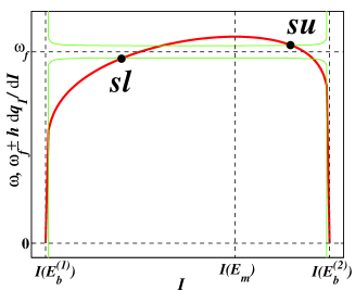
Figure 7: A schematic example illustrating the graphic solutions of Eqs. (15) for $n=1$, as intersections of the curve $\omega(I)$ (thick solid red line) with the curves $\omega_{f}\pm h{\rm d}q_{n}(I)/{\rm d}I$ (thin solid green lines). The solutions corresponding to the lower and upper relevant saddles (defined by Eq.(16)) are marked by dots and by the labels $sl$ and $su$ respectively (we do not mark other solutions because they are irrelevant).

Consider the stationary points corresponding to the remaining four roots of equations (15). As follows from the analysis of equations (14) linearized near the stationary points (cf. Chirikov:79 ; lichtenberg_lieberman ; Zaslavsky:1991 ; zaslavsky:1998 ; zaslavsky:2005 ; pr ), two of them are stable elliptic points crosses , often called nonlinear resonances, while two others are unstable hyperbolic points, often called saddles. These saddles are of main interest in the context of our work. They belong to the separatrices separating the regions of oscillations around the resonances from the regions of motion with a “running” slow angle $\tilde{\psi}$.

We shall distinguish the relevant saddles as the saddles with the lower action/energy (using the subscript “$sl$”) and upper action/energy (using the subscript “$su$”). The positions of the saddles in the $I-\tilde{\psi}$ plane are defined by the following equations (cf. Figs. 6 and 7):

$$g\equiv{\rm sign}(q_{n}(I_{su,sl}))=(-1)^{\left[\frac{n}{4}\right]},$$ (16)

$$\tilde{\psi}_{sl}=\pi(1+g)/2,\quad\quad\tilde{\psi}_{su}=\pi(1-g)/2,$$

$$X_{g}(I_{sl})=X_{-g}(I_{su})=0,$$

$$\frac{{\rm d}X_{g}(I_{sl})}{{\rm d}I_{sl}}>0,\quad\quad\frac{{\rm d}X_{-g}(I_{su})}{{\rm d}I_{su}}<0,$$

where $X_{\pm}(I)$ are defined in Eq. (15) while $I_{sl}$ and $I_{su}$ are closer to $I(E_{m})$ than any other solution of (16) (if any) from below and from above, respectively.

Given that the values of $h$ relevant to the minima of the spikes are small in the asymptotic limit $\Phi\rightarrow 0$, one may neglect the last term in the definition of $X_{\mp}$ in Eq. (15) in the lowest-order approximation, so that the equations $X_{\mp}=0$ reduce to the simple resonance condition

$$n\omega(I_{su,sl})=\omega_{f}.$$ (17)

Substituting here Eq. (7) for $\omega$, we obtain the explicit expressions for the energies in the saddles:

$$E_{su,sl}\approx\frac{1}{2}\pm\Delta E^{(1)},$$ (18)

$$\Delta E^{(1)}\equiv\sqrt{\Phi^{2}-64\exp\left(-\frac{n\pi}{\omega_{f}}\right)},\quad\quad\omega_{f}\leq n\omega_{m}.$$

The corresponding actions $I_{su,sl}$ are expressed via $E_{su,sl}$ by means of Eq. (13).

For $\omega_{f}\approx n\omega_{m}$, the values of $E_{su,sl}$ (18) lie in the range where the expression (12) for $q_{n}$ does hold true. This will be explicitly confirmed by the results of the calculations based on this assumption.

Using (16) for the angles and (18) for the energies, and the asymptotic expressions (7), (12) and (13) for $\omega(E)$, $q_{n}(E)$ and $I(E)$ respectively, and allowing for the resonance condition (17), we obtain explicit expressions for the values of the Hamiltonian (4) in the saddles:

$$\tilde{H}_{sl}=-\tilde{H}_{su}=\frac{\omega_{f}}{\pi}\left[2\Delta E^{(1)}-\Phi\ln\left(\frac{\Phi+\Delta E^{(1)}}{\Phi-\Delta E^{(1)}}\right)\right]+h\sqrt{2}.$$ (19)

As the analysis of simulations suggests (see the item 1 in the end of Sec. II) and as it is rigorously shown in the next subsection, one of the main conditions which should be satisfied in the spikes is the overlap in phase space between the separatrices of the nonlinear resonances, called separatrix reconnection pr ; Howard:84 ; Howard:95 . Given that the Hamiltonian $\tilde{H}$ is constant along any trajectory of the system (4), the values of $\tilde{H}$ in the lower and upper saddles of the reconnected separatrices are equal to each other:

$$\tilde{H}_{sl}=\tilde{H}_{su}\,,$$ (20)

that may be considered as the necessary and sufficient 27 condition for the reconnection. Taking into account that $\tilde{H}_{sl}=-\tilde{H}_{su}$ (see (19)), it follows from (20) that

$$\tilde{H}_{sl}=\tilde{H}_{su}=0.$$ (21)

Explicitly, the relations in (21) reduce to

$$h\equiv h(\omega_{f})=\frac{\omega_{f}}{\sqrt{2}\pi}\left[\Phi\ln\left(\frac{\Phi+\Delta E^{(1)}}{\Phi-\Delta E^{(1)}}\right)-2\Delta E^{(1)}\right],$$

$$\Delta E^{(1)}\equiv\sqrt{\Phi^{2}-64\exp(-\frac{n\pi}{\omega_{f}})},$$ (22)

$$0<\omega_{m}-\omega_{f}/n\ll\omega_{m}\equiv\frac{\pi}{2\ln(8/\Phi)},$$

$$n=1,3,5,...$$

The function $h(\omega_{f})$ (22) monotonously decreases to zero as $\omega_{f}$ grows from $0$ to $n\omega_{m}$, where the line abruptly stops. Fig. 10 shows the portions of the lines (22) relevant to the left wings of the 1st and 2nd spikes (for $\Phi=0.2$).

III.3 Barrier chaotic layers

The next step is to find a minimal value of $h$ for which the resonance separatrix overlaps the chaotic layer related to a potential barrier. With this aim, we study how the relevant outer boundary of the chaotic layer behaves as $h$ and $\omega_{f}$ vary. Assume that the relevant $\omega_{f}$ is close to $n\omega_{m}$ while the relevant $h$ is sufficiently large for $\omega(E)$ to be close to $\omega_{m}$ at all points of the outer boundary of the layer (the results will confirm these assumptions). Then the motion along the regular trajectory infinitesimally close to the layer boundary may be described within the resonance approximation (4). Hence the boundary may also be described as a trajectory of the resonant Hamiltonian (4). This is explicitly proved in the Appendix, using the separatrix map analysis that allows for the validity of the relation $\omega(E)\approx\omega_{m}$ for all $E$ relevant to the boundary of the chaotic layer. The main results are presented below. For the sake of clarity, we present them for each layer separately, although they are similar in practice.

III.3.1 Lower layer

Let $\omega_{f}$ be close to any of the spikes minima.

One of the key roles in the formation of the upper boundary of the layer is played by the angle-dependent quantity $\delta_{l}|\sin(\tilde{\psi})|$ which we call the generalized separatrix split (GSS) for the lower layer, alluding to the conventional separatrix split zaslavsky:1998 for the lower layer $\delta_{l}\equiv|\epsilon^{(low)}(\omega_{f})|h$ with $\epsilon^{(low)}$ given by Eq. (A11) melnikov . Accordingly, we use the term “lower GSS curve” for the following curve in the $I-\tilde{\psi}$ plane:

$$I=I_{\rm GSS}^{(l)}(\tilde{\psi})\equiv I(E_{b}^{(1)}+\delta_{l}|\sin(\tilde{\psi})|).$$ (23)

a. Relatively small $h$

If $h<h_{cr}^{(l)}(\omega_{f})$, where the critical value $\,h_{cr}^{(l)}(\omega_{f})\,$ is determined by Eq. (41) (its origin will be explained further), then there are differences in the boundary formation for the frequency ranges of odd and even spikes. We describe these ranges separately.

a.1. Odd spikes

In this case, the boundary is formed by the trajectory of the Hamiltonian (4) tangent to the GSS curve (see Fig. 16(a); cf. also Figs. 8(a), 9(b), 9(c)). There are two tangencies in the angle range $]-\pi,\pi[$: they occur at the angles $\pm\tilde{\psi}_{t}^{(l)}$ where $\tilde{\psi}_{t}^{(l)}$ is determined by Eq. (A21).

In the ranges of $h$ and $\omega_{f}$ relevant to the spike minimum, the asymptotic expressions for $\delta_{l}$ and $\tilde{\psi}_{t}^{(l)}$ are:

$$\delta_{l}=\sqrt{2}\pi h,$$ (24)

$$\tilde{\psi}_{t}^{(l)}=(-1)^{\left[\frac{n}{4}\right]}\sqrt{\frac{n\pi}{8\ln\left(1/\Phi\right)}}+\pi\frac{1-(-1)^{\left[\frac{n}{4}\right]}}{2}.$$ (25)

Hence, the asymptotic value for the deviation of the tangency energy $E_{t}^{(l)}$ from the lower barrier reduces to:

$$E_{t}^{(l)}-E_{b}^{(1)}\equiv\delta_{l}\sin(\tilde{\psi}_{t}^{(l)})=\frac{\pi^{3/2}}{2}\frac{h}{\sqrt{\ln\left(1/\Phi\right)/n}}.$$ (26)

The minimal energy on the boundary, $E_{\min}^{(l)}$, corresponds to $\tilde{\psi}=$ $0$ or $\pi$ for even or odd values of $[n/4]$ respectively. Thus, it can be found from the equality

$$\tilde{H}\left(I(E_{\min}^{(l)}),\tilde{\psi}=\pi(1-(-1)^{\left[\frac{n}{4}\right]})/2\right)=$$

$$=\tilde{H}\left(I_{t}^{(l)}\equiv I(E_{t}^{(l)}),\tilde{\psi}_{t}^{(l)}\right).$$ (27)

At $\Phi\rightarrow 0$, Eq. (III.3.1) yields the following expression for the minimal deviation of energy on the boundary from the barrier:

$$\delta_{\min}^{(l)} \equiv E_{\min}^{(l)}-E_{b}^{(1)}=(E_{t}^{(l)}-E_{b}^{(1)})/\sqrt{{\rm e}}=$$ (28)

$$= \frac{\pi^{3/2}}{2\sqrt{{\rm e}}}\frac{h}{\sqrt{\ln\left(1/\Phi\right)/n}}.$$

In the context of global chaos onset, the most important property of the boundary is that the maximal deviation of its energy from the barrier, $\delta_{\max}^{(l)}$, greatly exceeds both $\delta_{\min}^{(l)}$ and $\delta_{l}$. As $h\rightarrow h_{cr}^{(l)}$, the maximum of the boundary approaches the saddle “sl”.

a.2. Even spikes

In this case, the Hamiltonian (4) possesses saddles “s” in the close vicinity to the lower barrier (see Fig. 16(b)). Their angles differ by $\pi$ from those of “sl”:

$$\tilde{\psi}_{s}=\pi\frac{1-(-1)^{\left[\frac{n}{4}\right]}}{2}+2\pi m,$$ (29)

$$m=0,\pm 1,\pm 2,\ldots,$$

while the deviation of their energies from the barrier still lies in the relevant (resonant) range and reads, in the lowest-order approximation,

$$\delta_{s}=\frac{\pi}{2\sqrt{2}}\frac{h}{\ln(\ln(1/\Phi))}.$$ (30)

The lower whiskers of the separatrix generated by these saddles intersect the GSS curve while the upper whiskers in the asymptotic limit do not intersect it (Fig. 16(b)). Thus, it is the upper whiskers of the separatrix which form the boundary of the chaotic layer in the asymptotic limit. The energy on the boundary takes the minimal value right on the saddle “s”, so that

$$\delta_{\min}^{(l)}=\delta_{s}=\frac{\pi}{2\sqrt{2}}\frac{h}{\ln(\ln(1/\Phi))}.$$ (31)

Similar to the case of the odd spikes, the maximal (along the boundary) deviation of the energy from the barrier greatly exceeds both $\delta_{\min}^{(l)}$ and $\delta_{l}$. As $h\rightarrow h_{cr}^{(l)}$, the maximum of the boundary approaches the saddle “sl”.

b. Relatively large $h$

If $h>h_{cr}^{(l)}(\omega_{f})$, the previously described trajectory (the tangent one or the separatrix, for the odd or even spike ranges respectively) is encompassed by the separatrix of the lower nonlinear resonance and typically forms the boundary of the major stability island inside the lower layer (reproduced periodically in $\tilde{\psi}$ with the period $2\pi$). The upper outer boundary of the layer is formed by the upper part of the resonance separatrix. This may be interpreted as the absorption of the lower resonance by the lower chaotic layer.

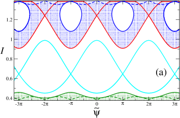
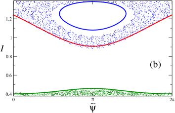
Figure 8: (a). Chaotic layers (shaded in green and blue, for the upper and lower layers respectively) in the plane of action $I$ and slow angle $\tilde{\psi}$, as described by our theory. Parameters are the same as in Figs. 5(b) and 6(b). The lower and upper boundaries of the figure box coincide with $I(E_{b}^{(1)})$ and $I(E_{b}^{(2)})$ respectively. The resonance separatrices are drawn by the cyan and red solid lines (for the lower and upper resonances respectively). Dashed green and blue lines mark the curves $I=I_{\rm GSS}^{(l)}(\tilde{\psi})\equiv I(E=E_{b}^{(1)}+\delta_{l}|\sin(\tilde{\psi})|)$ and $I=I_{\rm GSS}^{(u)}(\tilde{\psi})\equiv I(E=E_{b}^{(2)}-\delta_{u}|\sin(\tilde{\psi})|)$ respectively, where $\delta_{l}$ and $\delta_{u}$ are the values of the separatrix split related to the lower and upper barrier respectively. The upper boundary of the lower layer is formed by the trajectory of the resonant Hamiltonian system (4) tangent to the curve $I=I_{\rm GSS}^{(l)}(\tilde{\psi})$. The lower boundary of the upper layer is formed by the lower part of the upper (red) resonance separatrix. The periodic closed loops (solid blue lines) are the trajectories of the system (4) tangent to the curve $I_{\rm GSS}^{(u)}(\tilde{\psi})$: they form the boundaries of the major stability islands inside the upper chaotic layer. (b). Comparison of the chaotic layers obtained from computer simulations (dots) with the theoretically calculated boundaries (solid lines) shown in the box (a).

III.3.2 Upper layer

Let $\omega_{f}$ be close to any of the spikes minima.

One of the key roles in the formation of the lower boundary of the layer is played by the angle-dependent quantity $\delta_{u}|\sin(\tilde{\psi})|$ which we call the generalized separatrix split (GSS) for the upper layer; $\delta_{u}$ is the separatrix split for the upper layer: $\delta_{u}=|\epsilon^{(up)}(\omega_{f})|h$ with $\epsilon^{(up)}$ given by Eq. (A43). Accordingly, we use the term “upper GSS curve” for the following curve in the $I-\tilde{\psi}$ plane:

$$I=I_{\rm GSS}^{(u)}(\tilde{\psi})\equiv I(E_{b}^{(2)}-\delta_{u}|\sin(\tilde{\psi})|).$$ (32)

a. Relatively small $h$

If $h<h_{cr}^{(u)}(\omega_{f})$, where the critical value $\,h_{cr}^{(u)}(\omega_{f})\,$ is determined by Eq. (42) (its origin will be explained further), then there are some differences in the boundary formation in the frequency ranges of odd and even spikes: for odd spikes, the formation is similar to the one for even spikes in the lower-layer case and vice versa.

a.1. Odd spikes

In this case, the Hamiltonian (4) possesses saddles “$\tilde{s}$” in the close vicinity to the upper barrier, analogous to the saddles “s” near the lower barrier in the case of even spikes. Their angles are shifted by $\pi$ from those of “s”:

$$\tilde{\psi}_{\tilde{s}}=\tilde{\psi}_{s}+\pi=\pi\frac{1+(-1)^{\left[\frac{n}{4}\right]}}{2}+2\pi m,$$ (33)

$$m=0,\pm 1,\pm 2,\ldots$$

The deviation of their energies from the upper barrier coincides, in the lowest-order approximation, with $\delta_{s}$:

$$\delta_{\tilde{s}}=\delta_{s}=\frac{\pi}{2\sqrt{2}}\frac{h}{\ln(\ln(1/\Phi))}.$$ (34)

The upper whiskers of the separatrix generated by these saddles intersect the upper GSS curve while the lower whiskers in the asymptotic limit do not intersect it. Thus, it is the lower whiskers of the separatrix which form the boundary of the chaotic layer in the asymptotic limit. The deviation of energy from the upper barrier takes its minimal (along the boundary) value right on the saddle “$\tilde{s}$”,

$$\delta_{\min}^{(u)}=\delta_{\tilde{s}}=\frac{\pi}{2\sqrt{2}}\frac{h}{\ln(\ln(1/\Phi))}.$$ (35)

The maximal (along the boundary) deviation of the energy from the barrier greatly exceeds both $\delta_{\min}^{(u)}$ and $\delta_{u}$. As $h\rightarrow h_{cr}^{(u)}$, the maximum of the boundary approaches the saddle “su”.

a.2. Even spikes

The boundary is formed by the trajectory of the Hamiltonian (4) tangent to the GSS curve. There are two tangencies in the angle range $]-\pi,\pi[$: they occur at the angles $\pm\tilde{\psi}_{t}^{(u)}$ where $\tilde{\psi}_{t}^{(u)}$ is determined by Eq. (A41).

In the ranges of $h$ and $\omega_{f}$ relevant to the spike minimum, the expressions for $\delta_{u}$ and $\tilde{\psi}_{t}^{(u)}$ in the asymptotic limit $\Phi\rightarrow 0$ are similar to the analogous quantities in the lower-layer case:

$$\delta_{u}=\sqrt{2}\pi h,$$ (36)

$$\tilde{\psi}_{t}^{(u)}=-(-1)^{\left[\frac{n}{4}\right]}\sqrt{\frac{n\pi}{8\ln\left(\frac{1}{\Phi}\right)}}+\pi\frac{1+(-1)^{\left[\frac{n}{4}\right]}}{2}.$$ (37)

Hence, the asymptotic value for the deviation of the tangency energy $E_{t}^{(u)}$ from the upper barrier reduces to:

$$E_{b}^{(2)}-E_{t}^{(u)} = \delta_{u}\left|\pi\frac{1+(-1)^{\left[\frac{n}{4}\right]}}{2}-\tilde{\psi}_{t}^{(u)}\right|=$$ (38)

$$= \frac{\pi^{3/2}}{2}\frac{h}{\sqrt{\ln\left(1/\Phi\right)/n}}.$$

The maximal energy on the boundary, $E_{\max}^{(u)}$, corresponds to $\tilde{\psi}=\pi(1+(-1)^{[n/4]})/2$. Thus, it can be found from the equality

$$\tilde{H}(I=I(E_{\max}^{(u)}),\tilde{\psi}=\pi(1+(-1)^{[n/4]})/2)=$$

$$=\tilde{H}(I_{t}^{(u)}\equiv I(E_{t}^{(u)}),\tilde{\psi}_{t}^{(u)}).$$ (39)

At $\Phi\rightarrow 0$, Eq. (39) yields the following expression for the minimal (along the boundary) deviation of energy from the barrier:

$$\delta_{\min}^{(u)} \equiv E_{b}^{(2)}-E_{\max}^{(u)}=(E_{b}^{(2)}-E_{t}^{(u)})/\sqrt{{\rm e}}=$$ (40)

$$= \frac{\pi^{3/2}}{2{\rm e}^{1/2}}\frac{h}{\sqrt{\ln\left(1/\Phi\right)/n}}.$$

b. Relatively large $h$

If $h>h_{cr}^{(u)}(\omega_{f})$ (cf. Fig. 8(a)), the previously described trajectory (tangent one or the separatrix, for the even and odd spikes ranges respectively) is encompassed by the separatrix of the upper nonlinear resonance and typically forms the boundary of the major stability island inside the upper layer (reproduced periodically in $\tilde{\psi}$ with the period $2\pi$). The lower outer boundary of the layer is formed in this case by the lower part of the resonance separatrix. This may be interpreted as the absorption of the upper resonance by the upper chaotic layer.

The description of chaotic layers given above and, in more details, in the Appendix is the first main result of this paper. It provides a rigorous base for our intuitive assumption that the minimal value of $h$ at which the layers overlap corresponds to the reconnection of the nonlinear resonances with each other while the reconnected resonances touch one of the layers and touch/overlap another layer. It is remarkable also that we have managed to obtain the quantitative theoretical description of the chaotic layers boundaries in the phase space, including even the major stability islands, that well fits the results of simulations (see Fig. 8(b)).

III.4 Onset of global chaos: the spikes minima

The condition for the merger of the lower resonance and the lower chaotic layer may be written as

$$\tilde{H}(I=I(E=E_{b}^{(1)}+\delta^{(l)}_{\min}),\tilde{\psi}=0)=\tilde{H}_{sl}.$$ (41)

The condition for the merger of the upper resonance and the upper chaotic layer may be written as

$$\tilde{H}(I=I(E=E_{b}^{(2)}-\delta^{(u)}_{\min}),\tilde{\psi}=\pi)=\tilde{H}_{su}.$$ (42)

For the global chaos onset related to the spike minimum, either of Eqs. (41) and (42) should be combined with the condition of the separatrix reconnection (20). Let us seek first only the leading terms of $h_{s}\equiv h_{s}(\Phi)$ and $\omega_{s}\equiv\omega_{s}(\Phi)$. Then (20) may be replaced by its lowest-order approximation (21) or, equivalently, (22). Using also the lowest-order approximation for the barriers ($E_{b}^{(1,2)}\approx 1/2\mp\Phi$), we reduce Eqs. (41), (42) respectively to

$$\tilde{H}(I=I(E=1/2-\Phi+\delta^{(l)}_{\min}),\tilde{\psi}=0)=0,$$ (43)

$$\tilde{H}(I=I(E=1/2+\Phi-\delta^{(u)}_{\min}),\tilde{\psi}=\pi)=0,$$ (44)

where $\delta^{(l)}_{\min}$ is given by (28) or (31) for the odd or even spikes respectively while $\delta^{(u)}_{\min}$ is given by (35) or (40) for the odd or even spikes respectively.

The solution $(h_{s}^{(l)},\omega_{s}^{(l)})$ of the system of equations (22),(43) and the solution $(h_{s}^{(u)},\omega_{s}^{(u)})$ of the system of equations (22),(44) turn out identical to the leading order. For the sake of brevity, we derive below just $(h_{s}^{(l)},\omega_{s}^{(l)})$, denoting the latter, in short, as $(h_{s},\omega_{s})$ 28_prime .

The system of algebraic equations (22) and (43) is still too complicated to find its exact solution. However, we need only the lowest-order solution - and this simplifies the problem. Still, even this simplified problem is not trivial, both because the function $h_{s}(\Phi)$ turns out to be non-analytic and because $\Delta E^{(1)}$ in (22) is very sensitive to $\omega_{f}$ in the relevant range. Despite these difficulties, we have found the solution in a self-consistent way, as briefly described below.

Assume that the asymptotic dependence $h_{s}(\Phi)$ is:

$$h_{s}=a\frac{\Phi}{\ln(4{\rm e}/\Phi)}\,,$$ (45)

where the constant $a$ may be found from the asymptotic solution of (22), (43), (45).

Substituting the energies $E=1/2-\Phi+\delta^{(l)}_{\min}$ and $E=1/2+\Phi-\delta^{(u)}_{\max}$ in (7) and taking into account (28), (31), (35), (40) and (45), we find that, both for the odd and even spikes, the inequality

$$\omega_{m}-\omega(E)\ll\omega_{m}$$ (46)

holds in the whole relevant range of energies, i.e. for

$$\Delta E\in[-\Phi+\delta^{(l)}_{\min},\Phi-\delta^{(u)}_{\min}].$$ (47)

Thus, the resonant approximation is valid in the whole range (47). Eq. (12) for $q_{n}(E)$ is valid in the whole relevant range of energies too.

Consider Eq. (43) in a more explicit form. Namely, we express $\omega_{f}$ from (43), using Eqs. (4), (12), and (13), and using also (28)/(31) for odd/even spikes, and (45):

$$\omega_{f}=\frac{n\pi}{2\ln\left(\frac{4{\rm e}}{\Phi}\right)}\left\{1+\frac{h\sqrt{2}}{n\Phi}+O\left(\frac{1}{\ln^{2}(4{\rm e}/\Phi)}\right)\right\}.$$ (48)

We emphasize that the value of $\delta_{\min}^{(l)}$ enters explicitly only the term $O(\ldots)$ while, as it is clear from the consideration below, this term does not affect the leading terms in $(h_{s},\omega_{s})$. Thus, $\delta_{\min}^{(l)}$ does not affect the leading term of $\omega_{s}$ at all, while it affects the leading term of $h_{s}$ only implicitly: $\delta_{\min}^{(l)}$ lies in the range of energies where $nq_{n}(E)\approx\sqrt{2}$. This latter quantity is present in the second term in the curly brackets in (48) and, as it is clear from the further consideration, $h_{s}$ is proportional to it.

Substituting (48) into the expression for $\Delta E^{(1)}$ in (22), using (45) and keeping only the leading terms, we obtain

$$\Delta E^{(1)}=\Phi\sqrt{1-4{\rm e}^{c-2}},\quad\quad c\equiv\frac{2\sqrt{2}}{n}a.$$ (49)

Substituting $\Delta E^{(1)}$ from (49) into Eq. (22) for $h(\omega_{f})$ and allowing for (45) once again, we arrive at the transcendental equation for $c$:

$$\ln\left(\frac{1+\chi(c)}{1-\chi(c)}\right)-2\chi(c)=c,$$ (50)

$$\chi(c)\equiv\sqrt{1-4{\rm e}^{c-2}}.$$

The approximate numerical solution of Eq. (50) is:

$$c\simeq 0.179.$$ (51)

Thus, the final leading-order asymptotic formulas for $\omega_{f}$ and $h$ in the minima of the spikes are the following:

$$\omega_{s0}\equiv\omega_{s0}^{\left(\frac{n+1}{2}\right)}=n\frac{\pi}{2\ln\left(\frac{4{\rm e}}{\Phi}\right)},$$ (52)

$$h_{s0}\equiv h_{s0}^{\left(\frac{n+1}{2}\right)}=n\frac{c}{2\sqrt{2}}\frac{\Phi}{\ln\left(\frac{4{\rm e}}{\Phi}\right)},$$

$$n=1,3,5,...,\quad\quad\Phi\rightarrow 0,$$

where the constant $c\simeq 0.179$ is the solution of Eq. (50).

The rigorous derivation of the explicit asymptotic formulas for the minima of $h_{gc}(\omega_{f})$ is the second main result of this paper. These formulas allow one to immediately predict the parameters for the weakest perturbation which may lead to global chaos.

III.5 Numerical example and next-order corrections

For $\Phi=0.2$, the numerical simulations give the following values for the frequencies in the minima of the first two spikes (see Fig. 4):

$$\omega_{s}^{(1)}\approx 0.4005\pm 0.0005,\quad\quad\omega_{s}^{(2)}\approx 1.24\pm 0.005.$$ (53)

The values by the lowest-order formula (52) are:

$$\omega_{s0}^{(1)}\approx 0.393,\quad\quad\omega_{s0}^{(2)}\approx 1.18,$$ (54)

in rather good agreement with the simulations.

The next-order correction for $\omega_{s}$ can be immediately found from Eq. (48) for $\omega_{f}$ and Eq. (52) for $h_{s0}$, so that

$$\omega_{s1}\simeq\omega_{s0}(1+\frac{c}{2\ln\left(\frac{4{\rm e}}{\Phi}\right)})\approx\frac{n\pi\left(1+\frac{0.09}{\ln\left(\frac{4{\rm e}}{\Phi}\right)}\right)}{2\ln\left(\frac{4{\rm e}}{\Phi}\right)}\,,$$ (55)

$$n=1,3,5,...$$

The formula (55) agrees with the simulations even better than the lowest-order approximation:

$$\omega_{s1}^{(1)}\approx 0.402,\quad\quad\omega_{s1}^{(2)}\approx 1.21.$$ (56)

For $h$ in the spikes minima, the simulations give the following 26_prime values (see Fig. 4):

$$h_{s}^{(1)}\approx 0.0049,\quad\quad h_{s}^{(2)}\approx 0.03.$$ (57)

The values by the lowest-order formula (52) are:

$$h_{s0}^{(1)}\approx 0.0032,\quad\quad h_{s0}^{(2)}\approx 0.01.$$ (58)

The theoretical value $h_{s0}^{(1)}$ gives a reasonable estimate for the simulation value $h_{s}^{(1)}$. The theoretical value $h_{s0}^{(2)}$ gives the correct order of magnitude for the simulation value $h_{s}^{(2)}$. Thus, the accuracy of the lowest-order formula (52) for $h_{s}$ is much lower than that for $\omega_{s}$: this is due to the steepness of $h_{gc}(\omega_{f})$ in the ranges of spikes (the steepness, in turn, is due to the flatness of the function $\omega(E)$ near its maximum). Moreover, as the number of the spike $j$ increases, the accuracy of the lowest-order value $h_{s0}^{(j)}$ significantly decreases. The latter can be explained as follows. For the next-order correction to $h_{s0}^{(j)}$, the dependence on $\Phi$ reads as:

$$\frac{h_{s1}^{(j)}-h_{s0}^{(j)}}{h_{s0}^{(j)}}\propto\frac{1}{\ln(4{\rm e}/\Phi)}.$$ (59)

At least some of the terms of this correction are positive and proportional to $h_{s0}^{(j)}$ (e.g. due to the difference between the exact equation (15) and its approximate version (17)) while $h_{s0}^{(j)}$ is proportional to $n\equiv 2j-1$. Thus, for $\Phi=0.2$, the relative correction for the 1st spike is $\sim 0.25$ while the correction for the 2nd spike is a few times larger i.e. $\sim 1$. But the latter means that, for $\Phi=0.2$, the asymptotic theory for the 2nd spike cannot pretend to be a quantitative description of $h_{s}^{(2)}$, but only provide the correct order of magnitude. Besides, if $n>1$ while $\Phi$ exceeds some critical value, then the search of the minimum involves Eq. (66) rather than Eq. (20), as explained below in Sec. IV (cf. Figs. 10(b) and 11). Altogether, this explains why $h_{s}^{(1)}$ is larger than $h_{s0}^{(1)}$ only by 50$\%$ while $h_{s}^{(2)}$ is larger than $h_{s0}^{(2)}$ by 200$\%$.

The consistent explicit derivation of the correction to $h_{s0}^{(j)}$ is complicated. A reasonable alternative may be a proper numerical solution of the algebraic system of Eqs. (20) 32_prime and (41) for the odd spikes or (42) for the even spikes 28_prime ; 29_prime . To this end, in Eqs. (20) 32_prime and (41)/(42) we use: (i) the exact values of the saddle energies obtained from the exact relations (16) instead of the approximate relations (17); (ii) the exact formulas (5) and (6) for $\omega(E)$ instead of the asymptotic expression (7); (iii) the exact functions $q_{n}(E)$ instead of the asymptotic formula (12); (iv) the relation (27) and the calculation of the “tangent” state $(\tilde{\psi}_{t}^{(l)},I_{t}^{(l)})$ by Eqs. (A11), (A22) for the odd spikes, or relation (39) and the calculation of the “tangent” state $(\tilde{\psi}_{t}^{(u)},I_{t}^{(u)})$ by Eqs. (A41)-(A43) for the even spikes. Note that, to find the exact function $q_{n}(E)$, we substitute into the definition of $q_{n}(E)$ in (4) the explicit general_case solution for $q(E,\psi)$:

$$q(E,\psi)=\arcsin\left(\frac{\eta-\sqrt{2E}+\Phi}{1-\eta}\right)\quad{\rm for}\quad\psi\in\left[0,\frac{\pi}{2}\right],$$

$$q(E,\psi)=\pi-q(E,\pi-\psi)\quad\quad\quad\quad{\rm for}\quad\psi\in\left[\frac{\pi}{2},\pi\right],$$

$$q(E,\psi)=q(E,2\pi-\psi)\quad\quad\quad\quad\quad\quad{\rm for}\quad\psi\in\left[\pi,2\pi\right],$$

$$\eta\equiv\frac{1}{2}(\sqrt{2E}-\Phi+1){\rm sn}^{2}\left(\frac{2K}{\pi}\psi\right)\,,$$ (60)

where ${\rm sn}(x)$ is the elliptic sine Abramovitz_Stegun with the same modulus $k$ as the full elliptic integral $K$ defined in (5),(6).

The numerical solution described above gives:

$$\left(\omega_{s}^{(1)}\right)_{num}\approx 0.401\ ,\qquad\left(h_{s}^{(1)}\right)_{num}\approx 0.005\ ,$$

(61)

$$\left(\omega_{s}^{(2)}\right)_{num}\approx 1.24\ ,\qquad\left(h_{s}^{(2)}\right)_{num}\approx 0.052\ .$$

The agreement with the simulation results is: (i) excellent for $\omega_{s}$ for the both spikes and for $h_{s}$ for the 1st spike, (ii) reasonable for $h_{s}$ for the 2nd spike. Thus, if $\Phi$ is moderately small, a much more accurate prediction for $h_{s}$ than that by the lowest-order formula is provided by the numerical procedure described above.

IV THEORY OF THE SPIKES WINGS

The goal of this section is to find mechanisms responsible for the formation of the spikes wings (i.e. the function $h_{gc}(\omega_{f})$ in the ranges of $\omega_{f}$ slightly deviating from $\omega_{s}^{(j)}$) and to provide for their theoretical description.

Before developing the theory, we briefly analyze the simulation data (Fig. 4), concentrating on the 1st spike. The left wing of the spike is smooth and nearly straight. The initial part of the right wing is also nearly straight fluctuations though less steep. But, at some small distance from $\omega_{s}^{(1)}$, its slope changes jump-wise by a few times: compare the derivative fluctuations ${\rm d}h_{gc}/{\rm d}\omega_{f}\approx 0.1$ at $\omega_{f}$ slightly exceeding $\omega_{s}^{(1)}\approx 0.4$ (see the left inset in Fig. 4) and ${\rm d}h_{gc}/{\rm d}\omega_{f}\approx 0.4$ at $\omega_{f}=0.45\div 0.55$ (see the main part of Fig. 4). Thus, even prior to the theoretical analysis, one may assume that there are a few different important mechanisms responsible for the formation of the wings.

Consider the arbitrary $j$th spike. We have shown in the previous section that, in the asymptotic limit $\Phi\rightarrow 0$, the minimum of the spike corresponds to the intersection between the lines (20) and (41)/(42) for odd/even spikes. We recall that: (i) Eq. (20) corresponds to the overlap in phase space between nonlinear resonances of the same order $n\equiv 2j-1$; (ii) Eq. (41)/(42) corresponds to the onset of the overlap between the resonance separatrix associated with the lower/upper saddle and the chaotic layer associated with the lower/upper potential barrier; (iii) for $\omega_{f}=\omega_{s}^{(j)}$, the condition (41)/(42) guarantees also the overlap between the upper/lower resonance separatrix and the chaotic layer associated with the upper/lower barrier 28_prime .

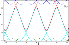
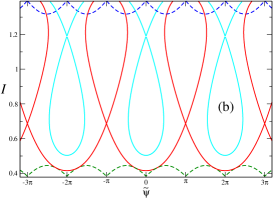
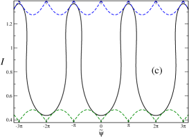
Figure 9: Illustrations of the mechanisms of the formation of the 1st spike wings and of the corresponding theoretical lines in Fig. 10(a). Boxes (a), (b) and (c) illustrate the lines by Eqs. (20), (41) and (64) respectively: the corresponding perturbation parameters are ($\omega_{f}=0.39,h=0.0077$), ($\omega_{f}=0.41,h=0.00598$) and ($\omega_{f}=0.43,h=0.01009$) respectively. Resonance separatrices are drawn by red and cyan. The dashed lines show the functions $I_{\rm GSS}^{(l)}(\tilde{\psi})$ and $I_{\rm GSS}^{(u)}(\tilde{\psi})$. The black line in (c) is the trajectory of the resonant Hamiltonian system (4) which is tangent to both dashed lines.

If $\omega_{f}$ becomes slightly smaller than $\omega_{s}^{(j)}$ the resonances shift closer to the barriers while moving apart from each other. Hence, as $h$ increases, the overlap of the resonances with the chaotic layers associated with the barriers occurs earlier than with each other. Therefore, at $0<\omega_{s}^{(j)}-\omega_{f}\ll\omega_{m}$, the function $h_{gc}(\omega_{f})$ should approximately correspond to the reconnection of resonances of the order $n\equiv 2j-1$ (Fig. 9(a)). Fig. 10(a) demonstrates that even the asymptotic formula (22) for the separatrix reconnection line fits the left wing of the 1st spike quite well while the numerically calculated line (20) agrees with the simulations perfectly.

If $\omega_{f}$ becomes slightly larger than $\omega_{s}^{(j)}$ then, on the contrary, the resonances shift closer to each other and more far from the barriers. Therefore, the overlap of resonances with each other occurs at smaller $h$ than the overlap between any of them and the chaotic layer associated with the lower/upper barrier (cf. Figs. 5(c) and 5(d) as well as 6(c) and 6(d)). Hence, it is the latter overlap which determines the function $h_{gc}(\omega_{f})$ in the relevant range of $\omega_{f}$ (Fig. 9(b)). Fig. 10 shows that $h_{gc}(\omega_{f})$ is indeed well approximated in the close vicinity to the right from $\omega_{s}^{(j)}$ by the numerical solution of Eq. (41)/(42) for an odd/even spike and, for the 1st spike and the given $\Phi$, even by its asymptotic form,

$$h\equiv h(\omega_{f})=$$ (62)

$$n\frac{-\Phi+\frac{\omega_{f}}{n\pi}\left[\Phi\left\{2\ln\left(\frac{4{\rm e}}{\Phi}\right)+\ln\left(\frac{\Phi+\Delta E^{(1)}}{\Phi-\Delta E^{(1)}}\right)\right\}-2\Delta E^{(1)}\right]}{2\sqrt{2}},$$

$$\Delta E^{(1)}\equiv\sqrt{\Phi^{2}-64\exp(-\frac{n\pi}{\omega_{f}})},$$

$$n\equiv 2j-1,\quad|\omega_{f}-\omega_{s}^{(j)}|\ll\omega_{m}\,,$$

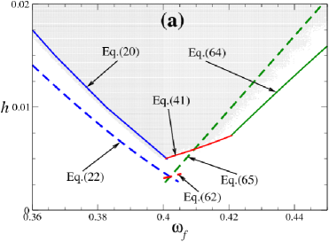
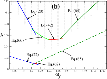
Figure 10: The 1st (a) and 2nd (b) spike in $h_{gc}(\omega_{f})$: comparison between the results of the numerical simulations (the lower boundary of the shaded area) and the theoretical estimates. The estimates are indicated by the corresponding equation numbers and are drawn by different types of lines, in particular the dashed lines represent the explicit asymptote for the solid line of the same color.

The mechanism described above determines $h_{gc}(\omega_{f})$ only in the close vicinity of $\omega_{s}^{(j)}$. If $\omega_{f}/n$ becomes too close to $\omega_{m}$ or exceeds it, then the resonances are not of immediate relevance: they may even disappear or, if they still exist, their closed loops shrink, so that they cannot anymore provide for the connection of the chaotic layers in the relevant range of $h$. At the same time, the closeness of the frequency to $\omega_{m}$ still may give rise to a large variation of action along the trajectory of the Hamiltonian system (4). For the odd/even spikes, the boundaries of the chaotic layers in the asymptotic limit $\Phi\rightarrow 0$ are formed in this case by the trajectory of (4) which is tangent to the lower/upper GSS curves (for the lower/upper layer) or by the lower/upper part of the separatrix of (4) generated by the saddle “$\tilde{s}$”/“$s$” (for the upper/lower layer). Obviously, the overlap of the layers occurs when these trajectories coincide with each other, that may be formulated as the equality of $\tilde{H}$ in the corresponding tangency and saddle:

$$\tilde{H}(I_{t}^{(l)},\tilde{\psi}_{t}^{(l)})=\tilde{H}(I_{\tilde{s}},\tilde{\psi}_{\tilde{s}})\quad{\rm for}\quad j=1,3,5,\ldots,$$

$$\tilde{H}(I_{s},\tilde{\psi}_{s})=\tilde{H}(I_{t}^{(u)},\tilde{\psi}_{t}^{(u)})\quad{\rm for}\quad j=2,4,6,\ldots,$$

$$I_{\tilde{s}}\equiv I(E_{b}^{(2)}-\delta_{\tilde{s}}),\quad\quad I_{s}\equiv I(E_{b}^{(1)}+\delta_{s}).$$ (63)

Note however that, for moderately small $\Phi$, the tangencies may be relevant both to the lower layer and to the upper one (see the Appendix). Indeed, such a case occurs for our example with $\Phi=0.2$: see Fig. 9(c). Therefore, the overlap of the layers corresponds to the equality of $\tilde{H}$ in the tangencies:

$$\tilde{H}(I_{t}^{(l)},\tilde{\psi}_{t}^{(l)})=\tilde{H}(I_{t}^{(u)},\tilde{\psi}_{t}^{(u)})\,.$$ (64)

To the lowest order, Eq. (63) and Eq. (64) read as:

$$h\equiv h(\omega_{f})=\frac{\sqrt{2}\Phi\ln\left(\frac{4{\rm e}}{\Phi}\right)}{\pi}\left(\omega_{f}-\frac{n\pi}{2\ln\left(\frac{4{\rm e}}{\Phi}\right)}\right).$$ (65)

Both the line (64) and the asymptotic line (65) well agree with the part of the right wing of the 1st spike situated beyond the immediate vicinity of the minimum from the right side, namely, to the right from the fold at $\omega_{f}\approx 0.42$ (Fig. 10(a)). The fold corresponds to the change of the mechanisms of the chaotic layers overlap.

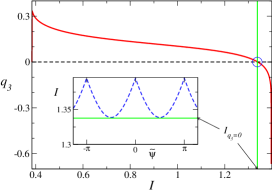
Figure 11: Amplitude of the 3rd Fourier harmonic as a function of action (solid red line). The dashed black line shows the zero level. Its intersection with the solid red line is marked by the circle. The green line indicates the value of action where $q_{3}=0$. The inset illustrates the line (66) in Fig. 10(b): the GSS curve touches the horizontal line $I=I_{q_{3}=0}$.

If $\Phi$ is moderately small while $n>1$, the description of the far wings by the numerical lines (20) and (64) may be still quite good but the asymptotic lines (22) and (65) cannot pretend to describe the wings quantitatively anymore (Fig. 10(b)). As for the very minimum of the spike and the wings in the close vicinity to it, one more mechanism may become relevant for their formation in this case (Figs. 10(b) and 11). This mechanism may be explained as follows. If $n>1$, then $q_{n}(E)$ becomes zero in the close vicinity ($\sim\Phi^{2}$) of the relevant barrier (the upper/lower barrier, in the case of even/odd spikes: cf. Fig. 11). As follows from the equations of motion (14), no trajectory can cross the line $I=I_{q_{n}=0}$. In the asymptotic limit $\Phi\rightarrow 0$, provided $h$ is from the relevant range, almost the whole GSS curve is farer from the barrier than the line $I=I_{q_{n}=0}$, and the latter becomes irrelevant. But, for a moderately small $\Phi$, the line may separate the whole GSS curve from the rest of the phase space. Then the resonance separatrix cannot connect to the GSS curve even if there is a state on the latter curve with the same value of $\tilde{H}$ as on the resonance separatrix. For a given $\omega_{f}$, the connection requires then a higher value of $h$: for such a value, the GSS curve itself crosses the line $I=I_{q_{n}=0}$. In the relevant range of $h$, the resonance separatrix passes very close to this line, so that the connection is well approximated by the condition that the GSS curve touches this line (see the inset in Fig. 11):

$$\delta_{u}=E_{b}^{(2)}-E_{q_{2j-1}=0}\quad\quad{\rm for}\quad j=2,4,6,\ldots,$$

(66)

$$\delta_{l}=E_{q_{2j-1}=0}-E_{b}^{(1)}\quad\quad{\rm for}\quad j=3,5,7,\ldots,$$

This mechanism is relevant for the formation of the minimum of the 2nd spike at $\Phi=0.2$, and in the close vicinity of the spike, on the left (Fig. 10(b)).

Finally, let us explicitly find the universal asymptotic shape of the spike in the vicinity of its minimum.

First, we note that the lowest-order expression (62) for the spike between the minimum and the fold can be written as the half-sum of the expressions (22) and (65) (which represent the lowest-order approximations for the spike to the left of the minimum, and to the right of the fold respectively). Thus, all three lines (22), (62) and (65) intersect in one point. The latter means that, in the asymptotic limit $\Phi\rightarrow 0$, the fold merges with the minimum: $\omega_{f}$ and $h$ in the fold asymptotically approach $\omega_{s}$ and $h_{s}$ respectively. Thus, though the fold is a generic feature of the spikes, it is not of main significance: the spike is formed basically by two straight lines. The ratio between their slopes is universal. So, introducing a proper scaling, we reduce the spike shape to a universal function (Fig. 12):

$$\tilde{h}(\Delta\tilde{\omega}_{f})=\tilde{h}^{(lw)}(\Delta\tilde{\omega}_{f})\equiv 1-\sqrt{1-4{\rm e}^{c-2}}\Delta\tilde{\omega}_{f}\approx$$

$$\quad\quad\quad\quad\quad\quad\quad\quad\approx 1-0.593\Delta\tilde{\omega}_{f}\quad{\rm for}\quad\Delta\tilde{\omega}_{f}<0,$$

$$\tilde{h}(\Delta\tilde{\omega}_{f})=\tilde{h}^{(rw)}(\Delta\tilde{\omega}_{f})\equiv 1+\Delta\tilde{\omega}_{f}\quad{\rm for}\quad\Delta\tilde{\omega}_{f}>0,$$

(67)

$$\tilde{h}^{(fold)}(\Delta\tilde{\omega}_{f})=\frac{\tilde{h}^{(lw)}(\Delta\tilde{\omega}_{f})+\tilde{h}^{(rw)}(\Delta\tilde{\omega}_{f})}{2}\equiv$$

$$\equiv 1+\frac{1-\sqrt{1-4{\rm e}^{c-2}}}{2}\Delta\tilde{\omega}_{f}\approx 1+0.203\Delta\tilde{\omega}_{f},$$

$$\tilde{h}\equiv\frac{h}{h_{s0}},\quad\quad\Delta\tilde{\omega}_{f}\equiv\frac{\omega_{f}-\omega_{s1}}{\omega_{s1}-\omega_{s0}},\quad\quad\Phi\rightarrow 0,$$

where $\omega_{s0}$ and $h_{s0}$ are the lowest-order expressions (52) respectively for the frequency and amplitude in the spike minimum, $\omega_{s1}$ is the expression (55) for the frequency in the spike minimum, including the first-order correction, and $c$ is the constant (51).

Beside the left and right wings of the universal shape (the solid lines in Fig. 12), we also present in (67) the function $\tilde{h}^{(fold)}(\Delta\tilde{\omega}_{f})$ (the dashed line in Fig. 12): it purposes to show that, on one hand, the fold asymptotically merges with the minimum but, on the other hand, the fold is generic and the slope of the spike between the minimum and the fold has a universal ratio to any of the slopes of the major wings.

Even for a moderately small $\Phi$, like in our example, the ratios between the three slopes related to the 1st spike in the simulations are reasonably well reproduced by those in Eq. (67): cf. Figs. 10(a) and 12. It follows from (67) that the asymptotic scaled shape is universal i.e. independent of $\Phi$, $n$ or any other parameter.

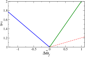
Figure 12: The universal shape of the spike minimum (67) (solid lines). The dashed line indicates the universal slope of the spike in between the minimum and the fold, which have merged in the universal (asymptotic) function (67).

The description of the wings of the spikes near their minima, in particular the derivation of the spike universal shape, is the third main result of this paper.

V GENERALIZATIONS AND APPLICATIONS

The new approach for the treatment of separatrix chaos opens a broad variety of important generalizations and applications, some of which are discussed below.

1. It may be applied to any separatrix layer, including in particular the conventional single-separatrix case. This is possible due to the characteristic dependence of the frequency of eigenoscillation on energy in the vicinity of any separatrix: the frequency keeps nearly a constant value even if the deviation of the energy from the separatrix strongly varies within a given scale of the deviation. To the best of our knowledge, the latter idea was not exploited before, which is why probably it was thought to be impossible to analyze the dynamics of the separatrix map in an explicit form. There were various estimates of the layer width in energy (see Chirikov:79 ; lichtenberg_lieberman ; Zaslavsky:1991 ; zaslavsky:1998 ; zaslavsky:2005 ; treshev and references therein) but the quantitative analysis of the layer boundaries in the phase space was never done in the non-adiabatic case. In contrast, our approach does analyze the dynamics of the separatrix map, and this allows us in particular to quantitatively describe the layer boundaries in case when the perturbation is resonant with the eigenoscillation in the relevant range of energy. It follows from such a description that, for a given small amplitude $h$ of the perturbation, the maximal layer width in energy is much larger than it is assumed by former theories (cf. Chirikov:79 ; lichtenberg_lieberman ; Zaslavsky:1991 ; zaslavsky:1998 ; zaslavsky:2005 where the maximal width is assumed to be $\sim h$). Thus, we can quantitatively describe large jumps and peaks of the layer width as a function of the perturbation amplitude and frequency respectively soskin2000 ; pr . Moreover, a rough estimate on the basis of our approach indicates that, for many classes of systems, the relative range of such jumps/peaks (i.e. the ratio between the upper and lower levels of the jump/peak) diverges in the asymptotic limit $h\rightarrow 0$.

2. Apart from the description of the boundaries, the approach allows us to describe the chaotic transport within the layer. In particular, it may allow us to calculate a positive Lyapunov exponent and to describe diffusion.

3. Our approach may be generalized for a non-resonant perturbation. The resonance approximation is not valid then but there still remains the property of a nearly constancy of the frequency of eigenoscillation within an arbitrary given scale of the deviation of energy from the separatrix. This property may allow us to explicitly describe the dynamics of the separatrix map for any frequency of perturbation which is less than or of the order of the resonance frequency.

4. Apart from Hamiltonian systems of the one and a half degrees of freedom and corresponding Zaslavsky separatrix maps, our approach may be useful in the treatment of other chaotic systems and separatrix maps (see treshev for the most recent major review on various types of separatrix maps and related continuous chaotic systems).

As concerns the facilitation of the global chaos onset between adjacent separatrices, we mention the following generalizations:

1. The spikes in $h_{gc}(\omega_{f})$ may occur for an arbitrary Hamiltonian system with two or more separatrices. The asymptotic theory can be generalized accordingly.

2. The absence of pronounced spikes at even harmonics $2j\omega_{m}$ is explained by the symmetry of the potential (1): the even Fourier harmonics of the coordinate, $q_{2j}$, are equal to zero. For time-periodic perturbation of dipole type, like in Eq. (2), there are no resonances of even order due to this symmetry Chirikov:79 ; lichtenberg_lieberman ; Zaslavsky:1991 ; zaslavsky:1998 ; zaslavsky:2005 ; pr . If either the potential is non-symmetric or the additive perturbation of the Hamiltonian is not an odd function of the coordinate, then even-order resonances do exist, resulting in the presence of the spikes in $h_{gc}(\omega_{f})$ at $\omega_{f}\approx 2j\omega_{m}$.

3. There may be an additional facilitation of global chaos onset which is reasonable to call a “secondary” facilitation. Let the frequency $\omega_{f}$ be close to the frequency $\omega_{s}$ of the spike minimum while the amplitude $h$ be $\sim h_{s}$ but still lower than $h_{gc}(\omega_{f})$. Then there are two resonance separatrices in the $I-\tilde{\psi}$ plane which are not connected by the chaotic transport (cf. Fig. 6(b) and 5(b)). This system possesses the zero-dispersion property. The trajectories of the resonant Hamiltonian (4) which start in between the separatrices oscillate in $I$ (as well as in ${\rm d}\tilde{\psi}/{\rm d}t$). The frequency $\tilde{\omega}$ of such oscillations along a given trajectory depends on the corresponding value of $\tilde{H}$ analogously to as $\omega$ depends on $E$ for the original Hamiltonian $H_{0}$: $\tilde{\omega}(\tilde{H})$ is equal to zero for the values of $\tilde{H}$ corresponding to the separatrices (being equal in turn to $\tilde{H}_{sl}$ and $\tilde{H}_{su}$: see Eq. (19)) while possessing a nearly rectangular shape in between, provided the quantity $|\tilde{H}_{sl}-\tilde{H}_{su}|$ is much smaller than the variation of $\tilde{H}$ within each of the resonances,

$$|\tilde{H}_{sl}-\tilde{H}_{su}|\ll\tilde{H}_{var}\sim|\tilde{H}_{sl}-\tilde{H}_{el}|\sim|\tilde{H}_{su}-\tilde{H}_{eu}|,$$ (68)

where $\tilde{H}_{el}$ and $\tilde{H}_{eu}$ are the values of $\tilde{H}$ in the elliptic point of the lower and upper resonance respectively. The maximum of $\tilde{\omega}(\tilde{H})$ in between $\tilde{H}_{sl}$ and $\tilde{H}_{su}$ is asymptotically described by the following formula:

$$\tilde{\omega}_{m}\approx\frac{\pi}{\ln\left(\tilde{H}_{var}/|\tilde{H}_{sl}-\tilde{H}_{su}|\right)}.$$ (69)

If we additionally perturb the system in such a way that an additional time-periodic term of the frequency $\tilde{\omega}_{f}\approx\tilde{\omega}_{m}$ arises in the resonance Hamiltonian, then the chaotic layers associated with the resonance separatrices may be connected by chaotic transport even for a rather small amplitude of the additional perturbation, due to a scenario similar to the one described in this paper.

There may be various types of such additional perturbation webs . For example, one may add to $H$ (2) one more dipole time-periodic perturbation of mixed frequency (i.e. $\approx\omega_{m}+\tilde{\omega}_{m}$). Alternatively, one may directly perturb the angle of the original perturbation by a low-frequency perturbation, i.e. the time-periodic term in $H$ (2) is replaced by the term

$$-hq\cos(\omega_{f}t+A\cos(\tilde{\omega}_{f}t)),$$ (70)

$$\omega_{f}\approx\omega_{m},\quad\quad\tilde{\omega}_{f}\approx\tilde{\omega}_{m}.$$

Recent physical problems where a similar situation is relevant are: chaotic mixing and transport in a meandering jet flow prants and reflection of light rays in a corrugated waveguide leonel .

4. If the time-periodic perturbation is multiplicative rather than additive, the resonances become parametric (cf. Landau:76 ). Parametric resonance is more complicated and much less studied than nonlinear resonance. Nevertheless, the main mechanism for the onset of global chaos remains the same, namely the combination of the reconnection between resonances of the same order and of their overlap in energy with the chaotic layers associated with the barriers. At the same time, the frequencies of the main spikes in $h_{gc}(\omega_{f})$ may change (though still being related to $\omega_{m}$). We consider below the example when the periodically driven parameter is the parameter $\Phi$ in (1) 37prime_new . The Hamiltonian reads as

$$H=p^{2}/2+(\Phi-\sin(q))^{2}/2,$$ (71)

$$\Phi=\Phi_{0}+h\cos(\omega_{f}t),\quad\quad\Phi_{0}={\rm const}<1.$$

The term $(\Phi-\sin(q))^{2}/2$ in $H$ (71) may be rewritten as $(\Phi_{0}-\sin(q))^{2}/2+(\Phi_{0}-\sin(q))h\cos(\omega_{f}t)+h^{2}\cos^{2}(\omega_{f}t)/2$. The last term in the latter expression does not affect the equations of motion. Thus, we end up with an additive perturbation $(\Phi_{0}-\sin(q))h\cos(\omega_{f}t)$. In the asymptotic limit $\Phi_{0}\rightarrow 0$, the $n$th-order Fourier component of the function $(\Phi_{0}-\sin(q))$ can be shown to differ from zero only for the orders $n=2,6,10,...$ Therefore one may expect the main spikes in $h_{gc}(\omega_{f})$ to be at frequencies twice larger than those for the dipole perturbation (2):

$$\omega_{sp}^{(j)}\approx 2\omega_{s}^{(j)}\approx 2(2j-1)\omega_{m},\quad\quad j=1,2,3,...$$ (72)

This well agrees with the results of simulations (Fig. 13).

Moreover, the asymptotic theory for the dipole perturbation may be immediately generalized to the present case: it is necessary only to replace the Fourier component of the coordinate $q$ by the Fourier component of the function $(\Phi_{0}-\sin(q))$:

$$(\Phi_{0}-\sin(q))_{n}=\left\{{}_{0\quad\quad{\rm at}\quad n\neq 2(2j-1),}^{\frac{4}{\pi n}\quad{\rm at}\quad n=2(2j-1),}\right.$$ (73)

$$j=1,2,3,...,$$

$$\Phi_{0}\rightarrow 0$$

(cf. Eq. (12) for $q_{n}$). We obtain:

$$\omega_{sp0}\equiv\omega_{sp0}^{\left(\frac{n+2}{4}\right)}=n\frac{\pi}{2\ln\left(\frac{4{\rm e}}{\Phi_{0}}\right)},$$ (74)

$$h_{sp0}\equiv h_{sp0}^{\left(\frac{n+2}{4}\right)}=n\frac{c\pi}{8}\frac{\Phi_{0}}{\ln\left(\frac{4{\rm e}}{\Phi_{0}}\right)},$$

$$n=2,6,10,...,\qquad\Phi_{0}\rightarrow 0,$$

where $c$ is given in Eqs. (50) and (51).

For $\Phi_{0}=0.2$, Eq. (74) gives, for the 1st spike, values differing from the simulation data by about $3\%$ for the frequency and by about $10\%$ for the amplitude. Thus, the lowest-order formulas accurately describe the 1st spike even for a moderately small $\Phi$.

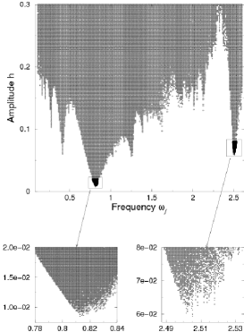
Figure 13: The diagram analogous to that one in Fig.4 but for the system (71) (with $\Phi_{0}=0.2$).

5. One more generalization relates to multi-dimensional Hamiltonian systems with two or more saddles with different energies: the perturbation may not necessarily be time-periodic, in this case. The detailed analysis will be done elsewhere.

Finally, we point out some analogy between the facilitation of global chaos onset described in our work and the so called stochastic percolation in 2D Hamiltonian systems described in percolation : the merging of internal and external chaotic zones is also relevant there, like in our case. However, both the models and the underlying mechanisms are very different. Namely, the problem studied in percolation is not of the zero-dispersion type; and the two-dimensionality is inherently important.

Let us turn now to a few detailed examples of applications of the facilitation of global chaos onset.

V.1 Electron gas in a magnetic superlattice, spinning pendulum, cold atoms in an optical lattice

The first application relates to a classical electron gas in a magnetic superlattice oleg98 ; oleg99 ; Oleg12 ; Oleg10 ; Shmidt:93 ; shepelyansky , where the electrons may be considered as non-interacting quasi-particles moving on a plane perpendicular to the magnetic field spatially periodic in one of the in-plane directions (we denote it as $x$-direction). Then the electron motion in the x-direction is described by the Hamiltonian (1) in which $q$ and $p$ are the scaled electron coordinate $x$ and generalized momentum $p_{x}$ respectively, while the parameter $\Phi$ is proportional to the reciprocal amplitude of the external magnetic field, $B^{-1}$, and to the generalized momentum $p_{y}$ in the second (perpendicular to $x$) in-plane direction: see for details pr ; oleg98 ; oleg99 . Note that $p_{y}$ remains constant during the motion oleg98 ; oleg99 .

If an AC electric field is applied in the $x$-direction, then the model (2)-(1) becomes relevant. The DC-conductivity in the $x$-direction is proportional to the fraction of electrons that can take part to the unbounded motion in the $x$-direction. This fraction, in turn, significantly grows as the range of energies involved in the unbounded chaotic transport increases oleg98 ; oleg99 .

If electrons move in vacuum vacuum , then it may be possible to inject a beam of electrons which possess the same velocity. In this case, the parameter $\Phi$ in the model (1) has some certain value, so that the results obtained in the previous sections are directly applicable. The spikes in $h_{gc}(\omega_{f})$ mean a drastic increase of the DC-conductivity occurring at a very weak amplitude of the AC electric field. The frequency of the AC field should be close to one of the spike frequencies. The effect is especially pronounced for the 1st spike i.e. when $\omega_{s}^{(1)}\approx\pi/[2\ln(4{\rm e}/\Phi)]$.

If the electron motion takes place in a semiconductor oleg98 ; oleg99 ; Oleg12 ; Oleg10 , then the velocity in the $y$-direction is necessarily statistically distributed. The same concerns the parameter $\Phi$ then. This might seem to smear the effect: cf. oleg98 where the conventional scenario of the onset of global chaos was exploited. However, in the case of the “zero-dispersion” scenario suggested in our paper, it typically should not be so. Indeed, a statistical distribution of the velocity typically decreases exponentially sharply as the velocity exceeds some characteristic value $v_{c}$: for high temperature $T$, the Boltzmann distribution of energy is relevant and, therefore, $v_{c}\propto\sqrt{T}$; for low temperatures, the Fermi distribution is relevant and, therefore, $v_{c}\propto\sqrt{E_{F}}$ where $E_{F}$ is the Fermi energy. On the other hand, in the range of small $\Phi$, the function $\ln(1/\Phi)$ does not significantly change even if $\Phi$ changes by a few times. Hence, if $\Phi_{c}\ll 1$ (where $\Phi_{c}$ denotes the $\Phi$ value corresponding to $v_{c}$), then the frequency $\omega_{s}^{(1)}$ of the partial (i.e. for a given value of $v_{y}$) 1st-order spike is nearly the same for most of the velocities in the relevant range $v_{y}\stackrel{{\scriptstyle<}}{{\sim}}v_{c}$, and it is approximately equal to $\omega_{c}\equiv\pi/[2\ln(4{\rm e}/\Phi_{c})]$. Similarly, $h_{s}^{(1)}\sim h_{c}\approx\omega_{c}\Phi_{c}/25$. Thus, as a function of $\omega_{f}$ for fixed $h\stackrel{{\scriptstyle>}}{{\sim}}h_{c}$, the DC-conductivity should have a sharp maximum for $\omega_{f}\approx\omega_{c}$.

If the parameter $\Phi$ is time-dependent (e.g. if the external magnetic field has an AC component or/and there is an AC electric force perpendicular to the $x$-direction), then the applications may be similar, with the only difference that the values of $\omega_{f}$ and $h$ in the minima of the main spikes differ from those for the additive perturbation, see Fig. 13 and the related discussion.

The results of the present paper may also be of direct relevance for a pendulum spinning about its vertical axis andronov , provided the friction is small. The periodic driving may be easily introduced mechanically, or electrically if the pendulum is electrically charged, or magnetically if the pendulum includes a ferromagnetic material.

Finally, we mention in this subsection that potentials similar to $U(q)$ (1), i.e. periodic potentials with two different-height barriers per period, may readily be generated for cold atoms by means of optical lattices 37prime . The dissipation may be suppressed by means of the detuning from the atomic resonance 37prime . Then the results of our paper are also of direct relevance to such systems.

V.2 Noise-induced escape

Consider the noise-induced escape over a potential barrier in the presence of a non-adiabatic periodic driving. For a moderately weak damping, such a driving decreases the activation barrier due to the resonant pushing the system in the range of resonant energies drsv . If the damping is even smaller, the decrease of the activation barrier becomes larger, due, however, to a different mechanism, typically related to the chaotic layer associated with the separatrix of the unperturbed system soskin2000 ; pr . The lower energy boundary of the layer is smaller than the potential barrier energy, so it is sufficient that the noise pulls the system right to this boundary (rather than to the very top of the potential barrier), after which the system may escape over the barrier purely dynamically. If the eigenfrequency as a function of the energy possesses a local maximum, then the effect may be even more pronounced iric ; pr : the decrease of the activation barrier may become comparable to the potential barrier at unusually small amplitudes of the driving, provided the driving frequency is close to the extremal eigenfrequency. One of the main mechanisms of the latter effect is closely related to phenomena discussed in the present paper. In the case of escape over two barriers of different heights, the effect should become even more pronounced due to the mechanism responsible for the spikes of $h_{gc}(\omega_{f})$ studied in the present paper. If the potential is periodic, e.g. like in optical lattices 37prime , the effect may lead to a drastic acceleration of the spatial diffusion.

V.3 Stochastic web

Our results may be applied to the stochastic web formation chernikov1 ; chernikov2 ; chernikov3 ; Zaslavsky:1991 . If a harmonic oscillator is perturbed by a plane wave whose frequency is equal to the oscillator eigenfrequency or its multiple, then the perturbation plays two roles chernikov2 ; Zaslavsky:1991 . On one hand, due to the resonance with the oscillator, it transforms the structure of the phase space of the oscillator, leading to an infinite number of cells divided by a unique separatrix. It has the form of a web of an infinite radius. On the other hand, the perturbation “dresses” this separatrix by an exponentially narrow chaotic layer (it is sometimes called “stochastic” layer). Such a web-like layer is called stochastic web. It may lead to chaotic transport of the system for rather long distances both in coordinate and in energy.

In case when either the resonance is not exact or/and the unperturbed oscillator possesses some nonlinearity, the perturbation generates many separatrices embedded into each other chernikov3 ; Zaslavsky:1991 rather than one single infinite web-like separatrix. Then a significant chaotic transport in energy may arise only if the magnitude of the perturbation exceeds some critical value corresponding to the overlap of chaotic layers associated, at least, with two neighbouring separatrices. And, still, the transport in energy remains limited since the width of the chaotic layer around each separatrix sharply decreases as the energy increases. It can be shown webs that some types of additional time-periodic perturbation lead to a low-frequency dipole perturbation of the resonance system (cf. the paragraph preceding Eq. (70)). The structure of separatrices in the reduced system possesses properties similar to that of the system considered in the present paper. Indeed, in the region between the separatrices, the resonance system performs regular oscillations, and the frequency of such oscillations, as function of the value of the resonance Hamiltonian, is equal to zero at each of the separatrices. Thus, it necessarily possesses a local maximum between energies corresponding to any two neighbouring separatrices, like in the case considered in the present paper. If the additional perturbation has an optimal frequency related to one of these local maxima, then the overlap of chaotic layers associated with neighbouring separatrices is greatly facilitated, similarly to the case considered in the present paper. Moreover, the local maximum of the eigenfrequency changes from pair to pair of separatrices weakly, so that if the magnitude of the auxiliary perturbation exceeds the critical value even slightly the simultaneous overlap between many chaotic layers may occur. Then, the distance of the chaotic transport in energy greatly increases.

Similar applications are relevant for the so called homogeneous (sometimes called periodic) stochastic webs chernikov1 ; Zaslavsky:1991 and many other web-like stochastic structures Zaslavsky:1991 .

Beside classical systems, stochastic webs may arise in quantum systems too. It was recently demonstrated, both theoretically Fromhold_PRL and experimentally Fromhold_Nature , that the stochastic web may play a crucial role in quantum electron transport in semiconductor superlattices subjected to stationary electric and magnetic fields. Due to the spatial periodicity with a period of about a few nanometers, the system possesses narrow minibands in the electron spectrum. It turns out that the description of the electron transport in the lowest miniband may be approximated by the model of a classical harmonic oscillator driven by a plane wave. The role of the harmonic oscillator is played by the cyclotron motion while the wave arises due to the interplay between the cyclotron motion and Bloch oscillations. If the cyclotron and Bloch frequencies are commensurate, then the phase space of such a system is threaded by a stochastic web. This gives rise to the delocalization of electron orbits, that leads in turn to a strong increase of the conductivity Fromhold_PRL ; Fromhold_Nature . However, this effect occurs only when the ratio between the electric and magnetic fields lies in the exponentially narrow regions corresponding to nearly integer ratios between the Bloch and cyclotron frequencies. The results of the present work suggest a method for a significant increase of the width of the relevant regions. If the cyclotron and Bloch frequencies are not exactly commensurate, then the stochastic web does not arise: rather a set of embedded separatrices arises provided the effective wave amplitude is sufficiently large. As discussed in the previous paragraph, even a rather weak time-periodic driving Fromhold_footnote of the optimal frequency may significantly increase the area of the phase space involved in the chaotic transport. This may provide for an effective control of the electron transport in such a system and may be used for developing electronic devices that exploit the intrinsic sensitivity of chaos (cf. Fromhold_Nature ). A similar effect may be used also to control transmission through other periodic structures, e.g. ultra-cold atoms in optical lattices Fromhold_Nature_20 ; Fromhold_Nature_21 ; Fromhold_Nature_29 and photonic crystals Fromhold_Nature_30 .

VI CONCLUSIONS

We have developed a new general approach for the treatment of separatrix chaos. This has allowed us to create a self-contained theory for the drastic facilitation of the global chaos onset between adjacent separatrices of a ID Hamiltonian system subject to a time-periodic perturbation. Both the new approach and the theory of the facilitation are closely interwoven in our paper but, at the same time, each of these two items is relevant even on its own. That is why we summarize them separately.

I. The new approach for separatrix chaos.

The approach is based on the separatrix map analysis which uses the characteristic property of the dependence of the frequency of eigenoscillation on energy in the vicinity of a separatrix: the frequency keeps nearly a constant value even if the deviation of the energy from the separatrix strongly varies within a given scale of the deviation. Due to this, the separatrix map evolves along the major part of the chaotic trajectory in regular-like way. The deviation of the chaotic trajectory from the separatrix may vary along the regular-like parts of the trajectory in a much wider range than along the irregular parts.

In the case of resonant perturbation, we match the separatrix map analysis and the resonant Hamiltonian approximation. This allows us in particular to find the boundaries of the chaotic layers in the phase space, which well agrees with computer simulations (Fig. 8). The latter theory has been successfully applied by us to the problem of the global chaos onset in the double-separatrix case, which is summarized in the item II below. Other applications and generalizations of the approach include in particular the following.

• It may be applied to the conventional single-separatrix case. In particular, our theory predicts that the maximal width of the separatrix chaotic layer in energy is typically $\gg h$, in contrast with former theories Chirikov:79 ; lichtenberg_lieberman ; Zaslavsky:1991 ; zaslavsky:1998 ; zaslavsky:2005 which assume that the maximal width is $\sim h$.

• It allows to analyze the transport within the layer.

• It may be generalized for a non-resonant perturbation and for a higher dimension.

II. The facilitation of the global chaos onset.

We have considered in details the characteristic example of a Hamiltonian system possessing two or more separatrices, subject to a time-periodic perturbation. The frequency $\omega$ of oscillation of the unperturbed motion necessarily possesses a local maximum $\omega_{m}$ as a function of energy $E$ in the range between the separatrices. It is smaller than the frequency $\omega_{0}$ of eigenoscillation in the stable state of the Hamiltonian system by a factor

$$R\sim\ln\left(\frac{1}{\Phi}\right),\quad\quad\Phi\equiv\frac{\Delta U}{U}\,,$$ (75)

where $\Delta U$ is the difference of the separatrices energies, while $U$ is the difference between the upper separatrix energy and the stable state energy.

If $\Phi\ll 1$, the function $\omega(E)$ is close to $\omega_{m}$ for most of the energy range between the separatrices: in the asymptotic limit $\Phi\rightarrow 0$, $\omega(E)$ approaches a rectangular form. Besides, the amplitude $q_{n}$ of the $n$th Fourier harmonic of the oscillation asymptotically approaches a non-small constant value in the whole energy range between separatrices. These two properties are responsible for most of the characteristic features of the global chaos onset in between the separatrices. The most striking one is a drastic facilitation of the global chaos onset when the perturbation frequency $\omega_{f}$ approaches $\omega_{m}$ or its multiples: the perturbation amplitude $h_{gc}$ required for global chaos possesses, as a function of the perturbation frequency $\omega_{f}$, deep spikes close to $\omega_{m}$ or its multiples.

On the basis of the theory for the boundaries of the chaotic layers, we have developed a self-consistent asymptotic theory for the spikes in the vicinity of the minima. In particular, the explicit asymptotic expressions for the very minima are given in Eqs. (52) and (55). The minimal amplitude $h_{gc}$ is smaller than the typical $h_{gc}$ for $\omega_{f}$ beyond the close vicinity of $\omega_{m}$ by a factor $\sim 10R\sim 10\ln(1/\Phi)$. The theory well agrees with the simulation results.

We have also found the mechanisms responsible for the spike wings (Figs. 9, 11). The theory well fits the simulations (Fig. 10). The asymptotic shape of the spike is universal: it is described by Eq. (67) (Fig. 12).

The facilitation of the global chaos onset may have the following applications in particular:

• drastic increase of the DC-conductivity of a 2D electron gas in a 1D magnetic superlattice;

• significant decrease of the activation barrier for noise-induced escape over double/multi-barrier structures, that may lead to a drastic acceleration of the diffusion in periodic structures;

• strong facilitation of the stochastic web formation.

VII ACKNOWLEDGMENTS

The work was partly supported by INTAS Grants 97-574 and 00-00867, by the Convention between the Institute of Semiconductor Physics and Pisa University for 2005-2007, and by the ICTP Program for Short-Term Visits. We are grateful to D. Escande, J. Meiss and G. Zaslavsky for discussions. SMS and RM acknowledge the hospitality of Pisa University and Institute of Semiconductor Physics respectively.

Appendix A Separatrix map analysis

The chaotic layers of the system (2) associated with the separatrices of the unperturbed system (1) are described here by means of the separatrix map. To derive the map, we follow the method described in Zaslavsky:1991 , but the analysis of the map significantly differs from existing ones lichtenberg_lieberman ; Zaslavsky:1991 ; zaslavsky:1998 ; zaslavsky:2005 ; treshev . It constitutes the method allowing to calculate chaotic layer boundaries in the phase space (rather than just in energy). It also allows to quantitatively describe the transport within the layer in a manner different from existing ones (cf. treshev ; vered and references therein).

We present below a detailed consideration of the lower chaotic layer while the upper layer may be considered similarly and we present just the results for it.

Figure 14: Schematic example of the time dependence of the velocity of the perturbed system (thick solid line) in the case when the energy of motion varies in the close vicinity of the top of the lower potential barrier. The dashed line marks the zero level of the velocity. Pulses of the velocity are schematically singled out by the parallelograms (drawn by a thin solid line). The two sequences of time instants $(...,t_{i-1},t_{i},t_{i+1},...)$ and $(...,t_{i-1}^{\prime},t_{i}^{\prime},t_{i+1}^{\prime},...)$ correspond to beginnings and centers of the pulses, respectively.

A.1 Lower chaotic layer

.

A.1.1 Separatrix map

The typical function $\dot{q}(t)$ for the trajectory close to the inner separatrix (the separatrix corresponding to the lower potential barrier) is shown in Fig. 14. One can resolve pulses in $\dot{q}(t)$. Each of them consists of two approximately antisymmetric spikes pulse . The pulses are separated by intervals during which $|\dot{q}|$ is relatively small. Generally speaking, successive intervals differ of each other. Let us introduce the pair of variables $\,E\,$ and $\,\varphi$:

$$E\equiv H_{0},\quad\varphi\equiv\omega_{f}t+\varphi_{a}\,,$$ (76)

where the constant $\varphi_{a}$ may be chosen arbitrarily.

The energy $E$ changes only during the pulses of $\dot{q}(t)$ and remains nearly unchanged during the intervals between the pulses, when $|\dot{q}(t)|$ is small Zaslavsky:1991 . We assign numbers $\,i\,$ to the pulses and introduce the sequences of $(E_{i},\varphi_{i})$ corresponding to initial instants of pulses $t_{i}$. In such a way, we obtain the following map (cf. Zaslavsky:1991 ):

$$E_{i+1}=E_{i}+\Delta E_{i},$$ (77)

$$\varphi_{i+1}=\varphi_{i}+\frac{\omega_{f}\pi(3-{\rm sign}(E_{i+1}-E_{b}^{(1)}))}{2\omega(E_{i+1})},$$

$$\Delta E_{i}\equiv h\int_{\hbox{\small{{\it i\,}th pulse}}}\!\!\!\!\!{\rm d}t\;\dot{q}(t)\cos(\omega_{f}t),$$

where $\,\int_{\hbox{\small{{\it i\,}th pulse}}}\,$ means integration over the $i$th pulse.

Before deriving a more explicit expression for $\Delta E_{i}$, we make two following remarks.

1. Let us denote with $t_{i}^{\prime}$ the instant within the $i$th pulse when $\dot{q}$ is equal to zero (Fig. 14). The function $\dot{q}(t-t_{i}^{\prime})$ is an odd function within the $i$th pulse and it is convenient to transform the cosine in the integrand in $\Delta E_{i}$ (A2) as

$$\cos(\omega_{f}t)\equiv\cos(\omega_{f}(t-t_{i}^{\prime})+\omega_{f}t_{i}^{\prime})\equiv$$

$$\cos(\omega_{f}(t-t_{i}^{\prime}))\cos(\omega_{f}t_{i}^{\prime})-\sin(\omega_{f}(t-t_{i}^{\prime}))\sin(\omega_{f}t_{i}^{\prime}),$$

and to put $\varphi_{a}=\omega_{f}(t_{i}^{\prime}-t_{i})$, so that $\varphi_{i}\equiv\omega_{f}t_{i}^{\prime}$.

2. Each pulse of $\dot{q}$ contains one positive and one negative spike. The first spike can be either positive or negative. If $E$ changes during the given $n$th pulse so that its value at the end of the pulse is smaller than $E_{b}^{(1)}$, then the first spikes of the $i$th and $(i+1)$st pulses have the same signs. On the contrary, if $E$ at the end of the $i$th pulse is larger than $E_{b}^{(1)}$, then the first spikes of the $i$th and $(i+1)$st pulses have opposite signs. Note that Fig. 14 corresponds to the case when the energy remains above $E_{b}^{(1)}$ during the whole interval shown in the figure. This obviously affects the sign of $\Delta E_{i}$, and it may be explicitly accounted for in the map if we introduce a new discrete variable $\sigma_{i}=\pm 1$ which characterizes the sign of $\dot{q}$ at the beginning of a given $i$th pulse,

$$\sigma_{i}\equiv{\rm sign}(\dot{q}(t_{i}))\ ,$$ (78)

and changes from pulse to pulse as

$$\sigma_{i+1}=\sigma_{i}\,{\rm sign}(E_{b}^{(1)}-E_{i+1})\ .$$ (79)

With account taken of the above remarks, we can rewrite the map (A2) as follows:

$$E_{i+1} = E_{i}+\sigma_{i}h\epsilon^{(low)}\sin(\varphi_{i}),$$ (80)

$$\varphi_{i+1} = \varphi_{i}+\frac{\omega_{f}\pi(3-{\rm sign}(E_{i+1}-E_{b}^{(1)}))}{2\omega(E_{i+1})},$$

$$\sigma_{i+1} = \sigma_{i}\,{\rm sign}(E_{b}^{(1)}-E_{i+1}),$$

$$\epsilon^{(low)} \equiv \epsilon^{(low)}(\omega_{f})=$$

$$= -\sigma_{i}\int_{i{\rm th}\;{\rm pulse}}{\rm d}t\;\dot{q}(t-t_{i}^{\prime})\sin(\omega_{f}(t-t_{i}^{\prime}))\approx$$

$$\approx -2\sigma_{i}\int_{t_{i}^{\prime}}^{t_{i+1}}{\rm d}t\;\dot{q}(t-t_{i}^{\prime})\sin(\omega_{f}(t-t_{i}^{\prime})).$$

The map similar to (A5) was introduced for the first time in ZF:1968 , and it is often called as the Zaslavsky separatrix map. Its mathematically rigorous derivation may be found e.g. in the recent major mathematical review treshev . The latter review describes also generalizations of the Zaslavsky map as well as other types of separatrix maps. The analysis presented below relates immediately to the Zaslavsky map but it is hoped to be possible to generalize it for other types of the separatrix maps too.

The variable $\epsilon^{(low)}$ introduced in (A5) will be convenient for the further calculations since it does not depend on $i$ in the lowest-order approximation. A quantity like $\delta_{l}\equiv h|\epsilon^{(low)}|$ is sometimes called the separatrix split zaslavsky:1998 since it is conventionally assumed that the maximal deviation of energy on the chaotic trajectory from the separatrix energy is of the order of $\delta_{l}$ lichtenberg_lieberman ; Zaslavsky:1991 ; zaslavsky:1998 ; zaslavsky:2005 . Though we shall also use this term, we emphasize that the maximal deviation may be much larger.

Dynamical chaos appears in the separatrix map (A5) because $\omega(E\rightarrow E_{b}^{(1)})\rightarrow 0$. Various heuristic criteria were suggested for the estimate of the chaotic layer width in energy lichtenberg_lieberman ; Zaslavsky:1991 ; zaslavsky:1998 ; zaslavsky:2005 . Frequencies relevant to our problem are much smaller than the reciprocal width of the spikes of $\dot{q}(t)$. For such frequencies, all these criteria lichtenberg_lieberman ; Zaslavsky:1991 ; zaslavsky:1998 ; zaslavsky:2005 give:

$$|E-E_{b}^{(1)}|\sim\frac{\omega_{f}}{\omega_{0}}h\left|\epsilon^{(low)}\right|,\quad\omega_{f}\ll\omega_{0}\approx 1,$$ (81)

where $\omega_{0}$ is the frequency of eigenoscillation at the bottom of the potential well.

The estimate (A6) was used in our earlier theory prl2003 . But we found later that, for the case of small $\omega_{f}$, the aforementioned criteria were insufficient, so that the estimate (A6) was incorrect to_be_published (cf. also E&E:1991 ; prl2005 ). Moreover, to search a uniform width of the layer is incorrect in cases like ours, where the width strongly depends on the angle. At the same time, the lowest-order formulas for the spike minimum $(h_{s},\omega_{s})$ are not affected by this, so that the results of prl2003 (with only the lowest-order formulas) are correct. Still, the higher-order corrections (quite significant for $h_{s}^{(j)}$ if $\Phi$ is moderately small) would be incorrect if they were calculated on the basis of the estimate (A6). Besides, the paper prl2003 did not address the intriguing question: why does even a small excess of $h$ over $h_{gc}(\omega_{f})$ result in the onset of chaos in a large part of the phase space between the separatrices, despite the fact that the width of the chaotic layers associated with the nonlinear resonances is exponentially small for $h=h_{gc}(\omega_{f})$? The analysis of the separatrix map presented below resolves these important problems.

In the adiabatic limit $\omega_{f}\rightarrow 0$, the excess of the upper boundary $E_{cl}^{(1)}$ of the lower layer over the lower barrier $E_{b}^{(1)}$ does not depend on angle and equals $2\pi h$ to_be_published (cf. also E&E:1991 ). But $\omega_{f}$ relevant for the spike of $h_{gc}(\omega_{f})$ cannot be considered as an adiabatic frequency, despite its smallness, because it is close to $\omega_{m}$ or to its multiple while all energies at the boundary lie in the range where the eigenfrequency is also close to $\omega_{m}$:

$$\omega_{f}\approx(2j-1)\omega_{m}\approx(2j-1)\omega(E_{cl}^{(1)}),$$ (82)

$$j=1,2,3,...$$

The validity of (A7) (confirmed by the results) is crucial for the description of the layer boundary in the relevant case.

A.1.2 Separatrix split

Let us explicitly evaluate $\epsilon^{(low)}$. Given that the energy is close to $E_{b}^{(1)}$, the velocity $\dot{q}(t-t_{i}^{\prime})$ in $\epsilon^{(low)}$ (A5) may be replaced by the corresponding velocity along the separatrix associated with the lower barrier, $\dot{q}_{s}^{(low)}(t-t_{i}^{\prime})$, while the upper limit in the integral may be replaced by infinity. Besides, in the asymptotic limit $\Phi\rightarrow 0$, the interval between spikes within the pulse becomes infinitely long pulse and, therefore, only short ($\sim\omega_{0}^{-1}$) intervals corresponding to the spikes contribute to the integral in $\epsilon^{(low)}$ (A5). In the scale $\omega_{f}^{-1}$, they may be considered just as two “instants”:

$$t_{sp}^{(1,2)}-t_{i}^{\prime}\approx\pm\frac{\pi}{4\omega_{m}},\quad\Phi\rightarrow 0.$$ (83)

In the definition of $\epsilon^{(low)}$ (A5), we substitute the argument of the sine by the corresponding constants for the positive and negative spikes respectively:

$$\epsilon^{(low)}\approx 2\sin\left(\frac{\pi\omega_{f}}{4\omega_{m}}\right)\int_{\rm positive\,spike}{\rm d}t\;\dot{q}_{s}^{(low)}(t-t_{i}^{\prime})$$

$$\quad\quad\approx 2\pi\sin\left(\frac{\pi\omega_{f}}{4\omega_{m}}\right),$$ (84)

$$\Phi\rightarrow 0.$$

In the derivation of the first equality in (A9), we have also taken into account that the function $\dot{q}_{s}^{(low)}(x)$ is odd. In the derivation of the second equality in (A9), we have taken into account that the right turning point of the relevant separatrix is the top of the lower barrier and the distance between this point and the left turning point of the separatrix approaches $\pi$ in the limit $\Phi\rightarrow 0$.

For the frequencies relevant to the minima of the spikes of $h_{gc}(\omega_{f})$, i.e. for $\omega_{f}=\omega_{s}^{(j)}\approx(2j-1)\omega_{m}$, we obtain:

$$\epsilon^{(low)}(\omega_{s}^{(j)})\approx 2\pi\sin\left((2j-1)\frac{\pi}{4}\right)=\sqrt{2}\pi(-1)^{\left[\frac{2j-1}{4}\right]},$$

$$j=1,2,3,...,\quad\Phi\rightarrow 0.$$ (85)

For moderately small $\Phi$, it is better to use the more accurate formula:

$$\epsilon^{(low)}(\omega_{f})=2\int_{0}^{\infty}{\rm d}t\;\dot{q}_{s}^{(low)}(t)\sin(\omega_{f}t),$$ (86)

where the instant $t=0$ corresponds to the turning point of the separatrix to the left from the lower barrier, i.e. $\dot{q}_{s}^{(low)}(t=0)=0$ while $\dot{q}_{s}^{(low)}>0$ for all $t>0$. The dependence $\left|\epsilon^{(low)}(\omega_{f})\right|$ by Eq. (A11) is shown for $\Phi=0.2$ in Fig. 15(a). For small frequencies, the asymptotic formula (A9) well fits the formula (A11).

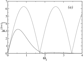
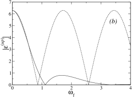
Figure 15: The theoretical estimates for the normalized separatrix split (for $\Phi=0.2$) as a function of the perturbation frequency, for the lower and upper layers in (a) and (b) respectively. The solid lines are calculated by Eqs. (A11) and (A43) (for (a) and (b) respectively) while dashed lines represent asymptotic expressions (A9) and (A44) respectively.

A.1.3 Dynamics of the map

Consider the dynamics of the map (A5), when $\omega_{f}$ is close to the spikes minima: $\omega_{f}\approx n\omega_{m}$ where $n\equiv 2j-1$ while $j=1,2,3,\ldots$. Let the energy at the step $i=-1$ be equal to $E_{b}^{(1)}$. The trajectory passing through the state with this energy is chaotic since $(\omega(E))^{-1}$ diverges as $E\rightarrow E_{b}^{(1)}$ and, therefore, the angle $\varphi_{-1}$ is not correlated with the angle on the previous step $\varphi_{-2}$. The quantity $\sigma_{-1}$ is not correlated with $\sigma_{-2}$ either. Thus, $\sin(\varphi_{-1})$ may take any value in the range $[-1,1]$ and $\sigma_{-1}$ may equally take the values 1 or -1. Therefore, the energy may change on the next step by an arbitrary value in the interval $[-h|\epsilon^{(low)}|,h|\epsilon^{(low)}|]$. Thus, $E_{0}-E_{b}^{(1)}$ may have a positive value $\sim h|\epsilon^{(low)}|$ except . Then, the approximate equality $n\omega(E_{0})\approx\omega_{m}$ holds, provided the value of $h$ is from the relevant range. Allowing for this and recalling that we are interested only in those realizations of the map such that $E_{0}>E_{b}^{(1)}$, the relevant realization of the map $i=-1\;\rightarrow\;i=0$ may be written as:

$$E_{0} = E_{b}^{(1)}+\sigma_{-1}h\epsilon^{(low)}\sin(\varphi_{-1})=$$

$$= E_{b}^{(1)}+h|\epsilon^{(low)}\sin(\varphi_{-1})|,$$

$$\varphi_{0} \approx \varphi_{-1}+n\pi,$$

$$\sigma_{0} =-\sigma_{-1}.$$ (87)

One may expect that the further evolution of the map will approximately follow, for some time, the trajectory of the system (4) with the initial energy $E_{0}$ (A12), and with an arbitrary $\varphi_{-1}$ and initial slow angle $\tilde{\psi}$ somehow related to $\varphi_{0}\approx\varphi_{-1}+n\pi$. Let us prove this explicitly.

Consider two subsequent iterations of the map (A5): $2i\rightarrow 2i+1$ and $2i+1\rightarrow 2i+2$ with an arbitrary $i\geq 0$. While doing this, we shall assume the validity of (A7) (it will be clarified below when this is true) from which it follows that: (i) $\omega(E_{k+1})\approx\omega(E_{k})$, (ii) $\varphi_{k+1}-\varphi_{k}\approx n\pi\equiv(2j-1)\pi$. It will follow from the results that the neglected corrections are small in comparison with the characteristic scales of the variation of $E$ and $\varphi$ (cf. the conventional treatment of the nonlinear resonance dynamics Chirikov:79 ; lichtenberg_lieberman ; Zaslavsky:1991 ; zaslavsky:1998 ; zaslavsky:2005 ; pr ). Besides, it follows from (A5) that, while the energy remains above the barrier energy, $\sigma_{k}$ oscillates, so that $\sigma_{2i}=\sigma_{0}$ and $\sigma_{2i+1}=-\sigma_{0}$. Then,

$$E_{2i+1} = E_{2i}+\sigma_{0}h\epsilon^{(low)}\sin(\varphi_{2i}),$$

$$\varphi_{2i+1} = \varphi_{2i}+\frac{\omega_{f}}{\omega(E_{2i+1})}\pi\approx$$ (88)

$$\approx \varphi_{2i}+n\pi+\pi\frac{\omega_{f}-n\omega(E_{2i})}{\omega(E_{2i})},$$

$$E_{2i+2} = E_{2i+1}-\sigma_{0}h\epsilon^{(low)}\sin(\varphi_{2i+1})=$$

$$= E_{2i+1}+\sigma_{0}h\epsilon^{(low)}\sin(\varphi_{2i+1}-n\pi)\approx$$

$$\approx E_{2i}+\sigma_{0}2h\epsilon^{(low)}\sin(\varphi_{2i}),$$

$$\varphi_{2i+2} = \varphi_{2i+1}+\frac{\omega_{f}}{\omega(E_{2i+2})}\pi\approx$$ (89)

$$\approx \varphi_{2i}+2\pi n+2\pi\frac{\omega_{f}-n\omega(E_{2i})}{\omega(E_{2i})}$$

(the second equality in the map for $E_{2i+2}$ takes into account that $n$ is odd so that $\sin(\varphi-n\pi)=-\sin(\varphi)$).

The quantity $\varphi_{2i+2}-\varphi_{2i}-2\pi n$ is small, so the map $2i\rightarrow 2i+2$ (A14) may be approximated by differential equations for $E_{2i}$ and $\tilde{\varphi}_{2i}\equiv\varphi_{2i}-2\pi ni$:

$$\frac{{\rm d}E_{2i}}{{\rm d}(2i)}=\sigma_{0}h\epsilon^{(low)}\sin(\tilde{\varphi}_{2i}),$$

$$\frac{{\rm d}\tilde{\varphi}_{2i}}{{\rm d}(2i)}=\frac{\pi}{\omega(E_{2i})}(\omega_{f}-n\omega(E_{2i})),$$ (90)

$$\tilde{\varphi}_{2i}\equiv\varphi_{2i}-2\pi ni.$$

Let us (i) use for $\epsilon^{(low)}$ the asymptotic formula (A10), (ii) take into account that the increase of $i$ by 1 corresponds to the increase of time by $\pi/\omega(E)$, and (iii) transform from the variables $(E,\tilde{\varphi})$ to the variables $(I,\tilde{\psi}\equiv n\pi(1-\sigma_{0})/2-\tilde{\varphi})$. Equations (A15) reduce then to:

$$\frac{{\rm d}I}{{\rm d}t}=-h\sqrt{2}(-1)^{\left[\frac{n}{4}\right]}\sin(\tilde{\psi}),$$

$$\frac{{\rm d}\tilde{\psi}}{{\rm d}t}=n\omega-\omega_{f},$$ (91)

$$\tilde{\psi}\equiv n\pi\frac{1-\sigma_{0}}{2}-\tilde{\varphi},\quad\quad n\equiv 2j-1.$$

Equations (A16) are identical to the equations of motion of the system (4) in the lowest-order approximation, i.e. to the equations (14) where $q_{n}$ is replaced by its asymptotic value (12) and the last term in the right-hand part of the second equation is neglected, being of higher order in comparison with the term $n\omega-\omega_{f}$.

Apart from the formal identity of Eqs. (A16) and (14), $\tilde{\psi}$ in (A16) and $\tilde{\psi}$ in (14) are identical to each other. Necessarily $t_{i}^{\prime}$ corresponds to a turning point (see Fig. 14) while the corresponding $\psi$ is equal to $2\pi i$ or $\pi+2\pi i$ for the right and left turning point respectively (see (4)) i.e. $\psi=2\pi i+\pi(1-\sigma_{i})/2$, so that $\tilde{\psi}_{(14)}\equiv n\psi-\omega_{f}t=n\pi(1-\sigma)/2-\tilde{\varphi}\equiv\tilde{\psi}_{(A16)}$.

The relevant initial conditions for (A16) follow from (A12) and from the relation between $\tilde{\psi}$ and $\varphi$:

$$I(0)=I(E=E_{b}^{(1)}+h\sqrt{2}\pi|\sin(\tilde{\psi}(0))|),$$ (92)

while $\tilde{\psi}(0)\equiv n\pi(1-\sigma_{0})/2-\varphi_{0}$ may be an arbitrary angle from the ranges where

$$(-1)^{[n/4]}\sin(\tilde{\psi}(0))<0.$$ (93)

For moderately small $\Phi$, it is better to use the more accurate dynamic equations (14) instead of (A16) and the more accurate initial value of action instead of (A17):

$$I(0)=I(E=E_{b}^{(1)}+\delta_{l}|\sin(\tilde{\psi}(0))|),\quad\quad\delta_{l}\equiv h|\epsilon^{(low)}|,$$ (94)

with $\epsilon^{(low)}$ calculated by (A11).

We name the quantity $\delta_{l}|\sin(\tilde{\psi})|$ the generalized separatrix split (GSS) for the lower layer. Unlike the conventional separatrix split $\delta_{l}$ zaslavsky:1998 , it is angle-dependent. The curve $I(\tilde{\psi})=I(E=E_{b}^{(1)}+\delta_{l}|\sin(\tilde{\psi})|)$ may be called then the GSS curve for the lower barrier and denoted as $I_{\rm GSS}^{(l)}(\tilde{\psi})$.

Finally, let us investigate an important issue: whether the transformation from the discrete separatrix map (i.e. (A13) and (A14)) to the differential equations (A15) is valid for the very first step and, if it is so, for how long it is valid after that. The transformation is valid as long as $\omega(E_{k})\approx n\omega_{f}$ i.e. as long as $E_{k}$ is not too close to the barrier energy $E_{b}^{(1)}$. At the step $k=0$, the system stays at the GSS curve, with a given (random) angle $\tilde{\psi}(0)$ from the range (A18). Thus, at this stage, the relation (A7) is certainly valid (for the relevant range of $h$ and for an angle a little away from the narrow vicinity of the multiples of $\pi$).

The change of energy at the next step is positive too:

$$E_{1}-E_{0} \equiv\sigma_{0}h\epsilon^{(low)}\sin(\tilde{\varphi}_{0})\approx$$

$$\approx-\sigma_{-1}h\epsilon^{(low)}\sin(\tilde{\varphi}_{-1}-n\pi)=$$

$$=\sigma_{-1}h\epsilon^{(low)}\sin(\tilde{\varphi}_{-1})\equiv E_{0}-E_{-1}>0.$$

This may also be interpreted as a consequence of the first equation in (A16) and of the inequality (A18).

Hence, (A7) is valid at the step $k=1$ too. Similarly, one can show that $E_{2}-E_{1}>0$, etc. Thus, the transformation (A13,A14)$\rightarrow$(A15) is valid at this initial stage indeed, and the evolution of $(E,\tilde{\varphi})$ does reduce to the resonant trajectory (14) with an initial angle from the range (A18) and the initial action (A19). This lasts until the resonant trajectory meets the GSS curve in the adjacent $\pi$ range of $\tilde{\psi}$ i.e. at $t$ such that the state $(I(t),\tilde{\psi}(t))$ satisfies the conditions:

$$I(t)=I_{\rm GSS}^{(l)}(\tilde{\psi}(t)),\quad\quad[\tilde{\psi}(t)/\pi]-[\tilde{\psi}(0)/\pi]=1.$$

At this instant, the absolute value of the change of energy $E_{k}$ in the separatrix map (A13) is equal to $E_{k}-E_{b}^{(1)}$ (just because the state belongs to the GSS curve) but the sign of this change is negative since the sign of $\sin(\varphi_{k})$ is opposite to the sign of $\sin(\varphi_{0})$. Therefore, at the step $k+1$, the system gets to the very separatrix, and the regular-like evolution stops: at the next step of the map, the system may either again get to the GSS curve with a new (random) angle from the range (A18) and start a new regular-like evolution as described above; or it may get to the similar GSS curve below the barrier and start an analogous regular-like evolution in the energy range below the barrier, until it stops in the same manner as described above, etc.

This approach makes it possible to describe all features of the transport within the chaotic layer. Their detailed description will be done elsewhere while, in the present context, it is most important to describe the upper outer boundary of the layer.

A.1.4 Boundary of the layer

We may now analyze the evolution of the boundary of the layer as $h$ grows. Some of the evolution stages are illustrated by Figs. 8, 9 and 16.

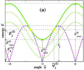
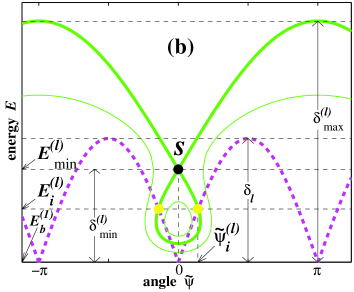
Figure 16: A schematic figure illustrating the formation of the boundary of the lower chaotic layer for $h<h_{cr}^{(l)}(\omega_{f})$ in the ranges of $\omega_{f}$ relevant to (a) odd, and (b) even spikes. The dashed magenta line shows the GSS curve in the energy-angle plane: $E(\tilde{\psi})=E_{\rm GSS}^{(l)}(\tilde{\psi})\equiv E_{b}^{(1)}+\delta_{l}|\sin(\tilde{\psi})|$. Green lines show examples of those trajectories (14) which have points in common with the GSS curve. One of such trajectories (14) (shown by the thick green line) forms the upper boundary of the lower chaotic layer: in (a), it is the trajectory tangent to the GSS curve; in (b), it is the upper part of the separatrix generated by the saddle “$s$”. Yellow dots indicate the relevant common points of the GSS curve and the thick green line. They have angles $\pm\tilde{\psi}_{t}^{(l)}$ and energy $E_{t}^{(l)}$ in the case (a), and angles $\pm\tilde{\psi}_{i}^{(l)}$ and energy $E_{i}^{(l)}$ in the case (b). The minimum and maximum deviation of energy on the boundary from the barrier energy are denoted as $\delta_{\min}^{(l)}$ and $\delta_{\max}^{(l)}$ respectively. The maximum deviation on the GSS curve is equal to $\delta_{l}$.

It follows from the analysis carried out in the previous subsection that any state (in the $I-\tilde{\psi}$ plane) lying beyond the GSS curve but belonging to any trajectory following the equations (14) which possesses common points with the GSS curve belongs to the chaotic layer: the system starting from such a state will get, sooner or later, to the separatrix, where the chaotization will necessarily occur. Therefore, the upper boundary of the chaotic layer coincides with the trajectory following the equations (14) with the initial action (A19) and an initial angle $\tilde{\psi}(0)$ from the range (A18) such that the trajectory deviates from the barrier energy more than a trajectory (14)-(A18)-(A19) with any other initial angle does. There may be only two topologically different options for such a trajectory: either it is the trajectory tangent to the GSS curve, or it is the separatrix trajectory which intersects the GSS curve (some schematic examples are shown in Figs. 16(a) and 16(b) respectively; some real calculations are shown in Figs. 8 and 9).

1. Relatively small $h$

Consider first values of $h$ which are large enough for the condition (A7) to be satisfied (the explicit criterion will be given in (A31)) but which are smaller than the value $h_{cr}^{(l)}\equiv h_{cr}^{(l)}(\omega_{f})$ determined by Eq. (41) (its meaning is explained below). The further analysis within this range of $h$ differs for the ranges of $\omega_{f}$ relevant to odd and even spikes, and we consider them separately.

A. Odd spikes

The relevant frequencies are:

$$\omega_{f}\approx n\omega_{m},\quad\quad n\equiv 2j-1,$$

$$j=1,3,5,\ldots$$ (95)

Let us seek the state $\{I_{t}^{(l)},\tilde{\psi}_{t}^{(l)}\}$ (with $\tilde{\psi}_{t}^{(l)}$ within the range $]0,\pi[$) where the resonant trajectory curve is tangent to the GSS curve. With this aim, we equal both the actions and the derivatives of both curves. The equality of actions immediately yields $I_{t}^{(l)}$ via $\tilde{\psi}_{t}^{(l)}$: $I_{t}^{(l)}\equiv I(E=E_{t}^{(l)})=I_{\rm GSS}^{(l)}(\tilde{\psi}_{t}^{(l)})$. The derivative along the GSS curve is obtained by differentiation of $I_{\rm GSS}^{(l)}(\tilde{\psi})$. The derivative along a resonant trajectory can be found dividing the first dynamic equation in (14) by the second one. Substituting the expression of $I_{t}^{(l)}$ via $\tilde{\psi}_{t}^{(l)}$ into the equality of the derivatives, we obtain a closed equation for $\tilde{\psi}_{t}^{(l)}$, and its solution immediately gives us the relevant $\tilde{\psi}(0)$:

$$\left[|\epsilon^{(low)}|\cos(\tilde{\psi}_{t}^{(l)})\left(1-\frac{\omega_{f}}{n\omega(E)}-h\frac{{\rm d}q_{n}(E)}{{\rm d}E}\cos(\tilde{\psi}_{t}^{(l)})\right)+\right.$$

$$\left.+q_{n}(E)\sin(\tilde{\psi}_{t}^{(l)})\right]_{E=E_{t}^{(l)}}=0,$$ (96)

$$E_{t}^{(l)}\equiv E_{b}^{(1)}+h|\epsilon^{(low)}|\sin(\tilde{\psi}_{t}^{(l)}),$$

$$\tilde{\psi}_{t}^{(l)}\in[0,\pi],\quad\quad n\equiv 2j-1,\quad\quad j=1,3,5,\ldots,$$

$$\tilde{\psi}(0)=\tilde{\psi}_{t}^{(l)}.$$

A careful analysis of the phase space structure shows that, in the present case (i.e. when $h<h_{cr}^{(l)}(\omega_{f})$ while $j$ is odd), there is no separatrix of the resonant Hamiltonian (4) which would both intersect the GSS curve and possess points above the tangent trajectory irrelevant . Thus, for this range of $h$, the outer boundary of the chaotic layer is formed by the trajectory following the dynamical equations (14) with the initial angle by (A22) and initial action (A19) (Fig. 16(a)).

Let us find the lowest-order solution of Eq. (A22). We neglect the term $1-\omega_{f}/(n\omega(E))$ (the result will confirm the validity of this) and use the lowest-order expression for the relevant quantities: namely, Eqs. (A10) and (12) for $\epsilon^{(low)}$ and $q_{n}$ respectively, and the lowest-order expression for ${\rm d}q_{n}/{\rm d}E$ which can be derived from Eq. (11):

$$\frac{{\rm d}q_{n}(E)}{{\rm d}E}=(-1)^{\left[\frac{n}{4}\right]}\frac{\pi}{4\sqrt{2}\left(E-E_{b}^{(1)}\right)\ln\left(\Phi^{-1}\right)},$$

$$n\equiv 2j-1,\quad\quad E-E_{b}^{(1)}\ll\Phi\rightarrow 0.$$ (97)

Then Eq. (A22) reduces to the following equation

$$\tan^{2}(\tilde{\psi}_{t}^{(l)})=\frac{n\pi}{8\ln\left(\Phi^{-1}\right)}.$$ (98)

The lowest-order solution of (A24) in the range $]0,\pi[$ reads as

$$\tilde{\psi}_{t}^{(l)}=(-1)^{\left[\frac{n}{4}\right]}\sqrt{\frac{n\pi}{8\ln(1/\Phi)}}+\pi\frac{1-(-1)^{\left[\frac{n}{4}\right]}}{2}.$$ (99)

It follows from the definition $E_{t}^{(l)}$ (A22) and from (A25) that the lowest-order expression for $E_{t}^{(l)}-E_{b}^{(1)}$ reads as

$$E_{t}^{(l)}-E_{b}^{(1)}=\delta_{l}\sin(\tilde{\psi}_{t}^{(l)})=\frac{\pi^{3/2}}{2}\frac{h}{\sqrt{\ln\left(1/\Phi\right)/n}}.$$ (100)

The next step is to find the minimal value of the energy on the boundary of the layer, $E_{\min}^{(l)}$. It follows from the analysis of the dynamical equations (14) that the corresponding angle $\tilde{\psi}_{\min}$ is equal to $0$ if ${\rm sign}(q_{2j-1})>0$ (i.e. $j=1,5,9,\ldots$) or to $\pi$ if ${\rm sign}(q_{2j-1})<0$ (i.e. $j=3,7,11,\ldots$): cf. Fig. 8(a). Given that the Hamiltonian (4) is constant along any trajectory (14) while the boundary coincides with one of such trajectories, the values of the Hamiltonian (4) in the states $\{I(E_{\min}^{(l)}),\tilde{\psi}=\tilde{\psi}_{\min}\}$ and $\{I_{t}^{(l)},\tilde{\psi}_{t}^{(l)}\}$ should be equal to each other. In the explicit form, this equality may be written as

$$\int_{E_{\min}^{(l)}}^{E_{t}^{(l)}}{\rm d}E\left(1-\frac{\omega_{f}}{n\omega(E)}\right)-$$ (101)

$$-h\left(q_{n}(E_{t}^{(l)})\cos(\tilde{\psi}_{t}^{(l)})-(-1)^{\left[\frac{n}{4}\right]}q_{n}(E_{\min}^{(l)})\right)=0.$$

Let us find the lowest-order solution of Eq. (A27). Assume that $E_{\min}^{(l)}$ still belongs to the range of $E$ where $\omega(E)\approx\omega_{m}$ (the result will confirm this assumption). Then the integrand in (A27) goes to zero in the asymptotic limit $\Phi\rightarrow 0$ and, hence, the integral may be neglected (the result will confirm the validity of this). The remaining terms in Eq. (A27) should be treated very carefully. In particular, it is insufficient to use the lowest-order value (12) for $q_{n}$ since it is the difference between $q_{n}(E_{t}^{(l)})$ and $q_{n}(E_{\min}^{(l)})$ that matters. Moreover, the approximate equality $q_{n}(E_{t}^{(l)})-q_{n}(E_{\min}^{(l)})\approx{\rm d}q_{n}(E_{t}^{(l)})/{\rm d}E_{t}^{(l)}(E_{t}^{(l)}-E_{\min}^{(l)})$ does not apply here either since, as it follows from Eq. (A23), the derivative ${\rm d}q_{n}(E)/{\rm d}E$ may strongly vary in the range $[E_{\min}^{(l)},E_{t}^{(l)}]$ if $(E_{t}^{(l)}-E_{\min}^{(l)})/(E_{\min}^{(l)}-E_{b}^{(1)})\stackrel{{\scriptstyle\sim}}{{>}}1$ (the result will show that it is the case). That is why it is necessary to use for $q_{n}$ the more accurate expression (11). Allowing for the asymptotic expression (A25) of $\tilde{\psi}_{t}^{(l)}$ and keeping only the lowest-order terms, one can finally reduce Eq. (A27) to the relation

$$\ln\left(\frac{E_{t}^{(l)}-E_{b}^{(1)}}{E_{\min}^{(l)}-E_{b}^{(1)}}\right)=\frac{1}{2}.$$ (102)

Substituting here the asymptotic value of $E_{t}^{(l)}$ (A26), we obtain the final lowest-order expression for the minimal (along the boundary) deviation of the energy from the barrier:

$$\delta_{\min}^{(l)} \equiv E_{\min}^{(l)}-E_{b}^{(1)}=(E_{t}^{(l)}-E_{b}^{(1)})/\sqrt{{\rm e}}=$$ (103)

$$= \frac{\pi^{3/2}}{2{\rm e}^{1/2}}\frac{h}{\sqrt{\ln\left(1/\Phi\right)/n}}.$$

It is necessary and sufficient that the condition $\omega(E)\approx\omega_{m}$ is satisfied at the minimal and maximal energies of the boundary to ensure that the second equality in (A7) holds true, i.e. that $\omega(E)$ is close to $\omega_{m}$ for all points of the boundary.

At the minimal energy, this condition reads as

$$\omega_{m}-\omega(E_{b}^{(1)}+\delta_{\min}^{(l)})\ll\omega_{m}.$$ (104)

Eq. (A30) determines the lower limit of the relevant range of $h$. The asymptotic form of (A30) is:

$$\frac{\ln\left(\frac{\Phi\sqrt{\ln(1/\Phi)}}{h}\right)}{\ln\left(1/\Phi\right)}\ll 1.$$ (105)

We emphasize that any $h$ of the order of $h_{s0}$ (52) satisfies this condition. In the asymptotic limit $\Phi\rightarrow 0$, the left-hand part of Eq. (A31) goes to zero.

As for the maximal energy, it may take values up to the energy of the lower saddle “$sl$”, i.e. $E_{sl}$ (18). Obviously, (A7) is valid at this saddle, too.

B. Even spikes

The relevant frequencies are:

$$\omega_{f}\approx n\omega_{m},\quad\quad n\equiv 2j-1,$$

$$j=2,4,6,\ldots$$ (106)

In this case, $q_{n}(E)$ and ${\rm d}q_{n}(E)/{\rm d}E$ have different signs for all $E$ within the relevant range (i.e. where $\omega(E)\approx\omega_{m}$, $q_{n}(E)\approx q_{n}(E_{m})$): cf. (12) and (A23). Then, in the asymptotic limit $\Phi\rightarrow 0$, Eq. (A22) for the tangency does not have any solution for $\tilde{\psi}_{t}^{(l)}$ in the relevant range 58_prime . There may be only solutions very close to some of $\pi$ integers, and the corresponding energies $E_{t}^{(l)}$ are very close to $E_{b}^{(1)}$ i.e. $\omega(E_{t}^{(l)})\ll\omega_{m}$: therefore they are irrelevant.

At the same time, unlike in the case of odd spikes, there exists a saddle with an angle

$$\tilde{\psi}_{s}^{(l)}=\pi\frac{1-(-1)^{\left[\frac{n}{4}\right]}}{2},$$ (107)

while the energy (which may be found as the appropriate solution of Eq. (15)) lies in the relevant vicinity of the lower barrier (Fig. 16(b)). In the lowest-order approximation, this saddle energy reads:

$$E_{s}^{(l)}\equiv E_{b}^{(1)}+\delta_{s},\quad\quad\delta_{s}=\frac{\pi}{2\sqrt{2}}\frac{h}{\ln(\ln(4{\rm e}/\Phi))}\;.$$ (108)

This saddle (denoted in Fig. 16(b) as “$s$”) generates a separatrix. Its upper whiskers go to the similar adjacent saddles (shifted in $\tilde{\psi}$ by $2\pi$). In the asymptotic limit $\Phi\rightarrow 0$, the upper whiskers are much steeper than the GSS curve and hence they do not intersect it 58_prime_prime . As concerns the lower whiskers, they do intersect the GSS curve and, moreover, two intersections lie in the relevant energy range (Fig. 16(b)). Let us show this explicitly. Let us write the expression for the Hamiltonian (4) in the relevant vicinity of the barrier energy (i.e. where $\omega_{m}-\omega(E)\ll\omega_{m})$, keeping, in the expression, both the lowest-order terms and the terms of next order (in particular, we use Eq. (11) for $q_{n}(E)$ and take into account that $0<\sqrt{2}-nq_{n}(E)\ll\sqrt{2}$ for the relevant range of $E$):

$$\tilde{H}(I=I(E=E_{b}^{(1)}+\delta),\tilde{\psi})=$$

$$=-\frac{n\delta\ln\left(\frac{2\Phi}{\delta}\right)}{2\ln\left(\frac{4{\rm e}}{\Phi}\right)}+\left(\omega_{f}-\frac{n\pi}{2\ln\left(\frac{4{\rm e}}{\Phi}\right)}\right)\frac{2\Phi}{\pi}\ln\left(\frac{4{\rm e}}{\Phi}\right)-$$

$$-(-1)^{\left[\frac{n}{4}\right]}h\sqrt{2}\left(1+\frac{n\pi\ln\left(\frac{2\Phi}{\delta}\right)}{8\ln\left(\frac{4{\rm e}}{\Phi}\right)}\right)\cos(\tilde{\psi}),$$ (109)

$$\omega_{m}-\omega(E+\delta)\ll\omega_{m}.$$

The Hamiltonian $\tilde{H}$ should possess equal values at the saddle “$s$” and at the intersections of the separatrix and the GSS curve. Let us denote the angle of the intersection in the range $]0,\pi[$ as $\tilde{\psi}_{i}^{(l)}$, and let us denote the deviation of its energy $E_{i}^{(l)}$ from $E_{b}^{(1)}$ as $\delta_{i}^{(l)}\equiv\delta_{l}\sin(\tilde{\psi}_{i}^{(l)})$.

Assuming that $|\tilde{\psi}_{i}^{(l)}-\tilde{\psi}_{s}^{(l)}|\ll 1$ (the result will confirm this) so that $\cos(\tilde{\psi}_{i}^{(l)})\approx(-1)^{[n/4]}(1-(\tilde{\psi}_{i}^{(l)}-\tilde{\psi}_{s}^{(l)})^{2}/2)\approx(-1)^{[n/4]}(1-(\delta_{i}^{(l)}/\delta_{l})^{2}/2)\approx(-1)^{[n/4]}(1-(\delta_{i}^{(l)}/h)^{2}/4)$, the equality of the values of $\tilde{H}$ reads as:

$$\frac{n}{2\ln\left(\frac{4{\rm e}}{\Phi}\right)}\left(\delta_{s}\ln\left(\frac{2\Phi}{\delta_{s}}\right)-\delta_{i}^{(l)}\ln\left(\frac{2\Phi}{\delta_{i}^{(l)}}\right)\right)=$$

$$=h\sqrt{2}\frac{n\pi}{8}\frac{\ln\left(\frac{\delta_{s}}{\delta_{i}^{(l)}}\right)}{\ln\left(\frac{4{\rm e}}{\Phi}\right)}-\frac{(\delta_{i}^{(l)})^{2}}{2\sqrt{2}h}.$$ (110)

Let us assume that, in the asymptotic limit $\Phi\rightarrow 0$, $\delta_{i}^{(l)}\ll\delta_{s}$ (the result will confirm this). Then the left-hand part is asymptotically smaller than the first term in the right-hand part. So, Eq. (A36) implies, in the asymptotic limit, that the right-hand side equals zero. Expressing $h$ via $\delta_{s}$ from Eq. (A34), we finally obtain a closed transcendental equation for $\delta_{s}/\delta_{i}^{(l)}$:

$$\left(\frac{\delta_{s}}{\delta_{i}^{(l)}}\right)^{2}\ln\left(\frac{\delta_{s}}{\delta_{i}^{(l)}}\right)=$$

$$=\frac{\pi\ln\left(\frac{4{\rm e}}{\Phi}\right)}{n\left(\ln\left(\ln\left(\frac{4{\rm e}}{\Phi}\right)\right)\right)^{2}}\equiv A.$$ (111)

In the asymptotic limit $\Phi\rightarrow 0$, the quantity $A$ diverges and, hence, the lowest-order asymptotic solution of Eq. (A37) reads as

$$\frac{\delta_{s}}{\delta_{i}^{(l)}}=\sqrt{\frac{2A}{\ln(A)}}.$$ (112)

Substituting here the expression (A34) for $\delta_{s}$ and the expression (A37) for $A$, we obtain:

$$\delta_{i}^{(l)}=h\frac{1}{4}\sqrt{\frac{n\pi\ln\left(\ln\left(\frac{4{\rm e}}{\Phi}\right)\right)}{\ln\left(\frac{4{\rm e}}{\Phi}\right)}}.$$ (113)

Thus, we have proved the following asymptotic properties of the separatrix generated by the saddle “$s$”: 1) the lower whiskers of the separatrix do intersect the GSS curve in the relevant range of $E$ (i.e. where the resonant approximation is valid), 2) the upper whiskers of the separatrix do not intersect the GSS curve (there is no solution of Eq. (A36) in the range $\delta_{i}^{(l)}>\delta_{s}$). The former property confirms the self-consistence of the asymptotic theory for even spikes; the latter property means that the upper outer boundary of the lower chaotic layer is formed by the upper whiskers of the separatrix generated by the saddle “$s$”.

Finally, we explicitly note that the minimal (along the boundary) deviation of energy from the barrier energy occurs occurs right at the saddle “$s$”, i.e.

$$\delta_{\min}^{(l)}=\delta_{s}.$$ (114)

2. Relatively large $h$.

As $h$ grows, the boundary of the layer raises up while the lower part of the resonance separatrix, on the contrary, goes down. They reconnect at the critical value of $h$, $h_{cr}^{(l)}\equiv h_{cr}^{(l)}(\omega_{f})$, determined by Eq. (41), that may be considered as the absorption of the resonance by the chaotic layer. If $h$ grows further, then the GSS curve and the resonance separatrix intersect. As a result, the trajectory starting from the state with the angle (A22) and action (A19), for odd spikes, or from the saddle “$s$”, for even spikes, is encompassed by the resonance separatrix. So, it does not form the outer boundary of the layer anymore. Rather it forms the inner boundary i.e. the boundary of the main island of the stability inside the layer, repeated periodically in $\tilde{\psi}$ with a period $2\pi$ (cf. analogous islands in the upper layer in Fig. 8). Unless the lower chaotic layer reconnects with the upper one, the outer boundary of the lower layer is formed by the upper part of the resonance separatrix. The relevant initial angle $\tilde{\psi}(0)$ on the GSS curve corresponds to the intersection of the GSS curve with the resonance separatrix (cf. the analogous situation for the upper layer in Fig. 8).

A.2 Upper chaotic layer

The upper chaotic layer may be treated analogously footnote_divergence to the lower layer. We present here only the results.

Similarly to the lower-layer case, one may consider the ranges of relatively small $h$ (namely, smaller than $h_{cr}^{(u)}\equiv h_{cr}^{(u)}(\omega_{f})$ determined by Eq. (42)) and relatively large $h$ (i.e. $h>h_{cr}^{(u)}$). In the former range, the formation of the boundary occurs in a manner which is, in a sense, opposite to that for the lower-layer case. For even spikes, the lower outer boundary is formed by tangency while, for odd spikes, it is formed by the lower part of the separatrix generated by the saddle “$\tilde{s}$”, analogous to the saddle “$s$”in the lower-layer case 59_prime .

So, for even spikes, the angle of tangency $\tilde{\psi}_{t}^{(u)}$ is determined by the following equation

$$\left[|\epsilon^{(up)}|\cos(\tilde{\psi}_{t}^{(u)})\left(1-\frac{\omega_{f}}{n\omega(E)}-h\frac{{\rm d}q_{n}(E)}{{\rm d}E}\cos(\tilde{\psi}_{t}^{(u)})\right)-\right.$$

$$\left.-q_{n}(E)\sin(\tilde{\psi}_{t}^{(u)})\right]_{E=E_{t}^{(u)}}=0,$$ (115)

$$E_{t}^{(u)}\equiv E_{b}^{(2)}-h|\epsilon^{(up)}|\sin(\tilde{\psi}_{t}^{(u)})$$

$$\tilde{\psi}_{t}^{(u)}\in\left[0,\pi\right],\quad\quad n\equiv 2j-1,\quad\quad j=2,4,6,\ldots,$$

$$\tilde{\psi}(0)=\tilde{\psi}_{t}^{(u)},$$

and $\tilde{\psi}_{t}^{(u)}$ determines the tangency energy:

$$E_{t}^{(u)}=E_{b}^{(2)}-h|\epsilon^{(up)}|\sin(\tilde{\psi}_{t}^{(u)}),$$ (116)

where the quantity $\epsilon^{(up)}$ is described by the formula

$$\epsilon^{(up)}(\omega_{f})=2\int_{0}^{\infty}{\rm d}t\;\dot{q}_{s}^{(up)}(t)\cos(\omega_{f}t)\,,$$ (117)

where $\dot{q}_{s}^{(up)}(t)$ is the time dependence of the velocity along the separatrix associated with the upper barrier and the instant $t=0$ is chosen so that $q_{s}^{(up)}(t=0)$ is equal to the coordinate of the lower barrier while $\dot{q}_{s}^{(up)}>0$ for $t\in[0,\infty[$. The dependence $\left|\epsilon^{(up)}(\omega_{f})\right|$ in Eq. (A43) is shown for $\Phi=0.2$ in Fig. 15(b).

The asymptotic form of Eq. (A43) reads as

$$\epsilon^{(up)}\equiv\epsilon^{(up)}(\omega_{f})=2\pi\cos\left(\frac{\pi\omega_{f}}{4\omega_{m}}\right)\,.$$ (118)

For $\omega_{f}=\omega_{s}^{(j)}\approx(2j-1)\omega_{m}$, Eq. (A43) reduces to

$$\epsilon^{(up)}(\omega_{s}^{(j)})\approx 2\pi\cos\left((2j-1)\frac{\pi}{4}\right)=\sqrt{2}\pi(-1)^{\left[\frac{2j+1}{4}\right]},$$

$$j=1,2,3,...,\quad\Phi\rightarrow 0.$$ (119)

The lowest-order solution of (A41) is given in Eq. (37), so that $E_{t}^{(u)}$ is approximated by Eq. (38). The maximal energy on the lower boundary of the layer corresponds to $\tilde{\psi}(t)=\pi$ if $j=2,6,10,\ldots$ or $0$ if $j=4,8,12,\ldots$ and is determined by Eq. (39). The asymptotic value of the minimal deviation from the upper barrier of the energy at the boundary, $\delta_{\min}^{(u)}$, is given in Eq. (40).

For odd spikes, the boundary is formed by the lower part of the separatrix generated by the saddle “$\tilde{s}$ ”. The angle of the saddle is given in Eq. (33) while the deviation of its energy from the barrier is approximated, to the lowest-order approximation, by Eq. (34).

As $h$ grows, the boundary of the layer goes down while the upper part of the upper resonance separatrix goes up. They reconnect at $h=h_{cr}^{(u)}\equiv h_{cr}^{(u)}(\omega_{f})$, as determined by Eq. (42), that may be considered as the absorption of the resonance by the chaotic layer.

For larger $h$, the boundary of the layer is formed by the lower part of the upper resonance separatrix (Fig. 8), unless the latter intersects the lower GSS curve (in the latter case, $h_{cr}^{(u)}$ marks the global chaos onset).

References

- (1) B.V. Chirikov, Phys. Rep. 52, 263 (1979).
- (2) A.J. Lichtenberg and M.A. Liebermann, Regular and Stochastic Motion (Springer, New York, 1992).
- (3) G.M. Zaslavsky, R.D. Sagdeev, D.A. Usikov and A.A. Chernikov, Weak Chaos and Quasi-Regular Patterns (Cambridge University Press, 1991).
- (4) G.M. Zaslavsky, Physics of Chaos in Hamiltonian systems (Imperial Colledge Press, 1998).
- (5) G.M. Zaslavsky, Hamiltonian Chaos and Fractional Dynamics (Oxford University Press, 2005).
- (6) S.M. Soskin, R. Mannella, P.V.E. McClintock, Phys. Rep. 373, 247 (2003).
- (7) J.E. Howard and S.M. Hohs, Phys. Rev. A 29, 418 (1984); D. del-Castillo-Negrete, J.M. Greene, P.J. Morrison, Physica D 61, 1 (1996); H. R. Dullin, J. D. Meiss, D. Sterling, Nonlinearity 13, 203 (2000); A.D. Morozov, Chaos 12, 539 (2002).
- (8) J.E. Howard, J. Humpherys, Physica D 80, 256 (1995).
- (9) More complicated cases are considered e.g. in pr ; Howard:95 .
- (10) This overlap is often called the separatrix reconnection pr ; Howard:84 ; Howard:95 .
- (11) D.G. Luchinsky, P.V.E. McClintock, S.M. Soskin, N.D. Stein, A.B. Neiman, Phys. Rev. E 53, 4240 (1996).
- (12) S.M. Soskin, O.M. Yevtushenko, and R. Mannella, Phys. Rev. Lett. 90, 174101 (2003).
- (13) S.M. Soskin, O.M. Yevtushenko, and R. Mannella, in Noise in Complex Systems and Stochastic Dynamics II, eds. Z. Gingl, J.M. Sancho, L. Schimansky-Geier, J. Kertesz, Proceedings of SPIE Vol. 5471 (SPIE, Bellingham, WA, 2004) p. 355.
- (14) A.A. Andronov, A.A. Vitt, S.E. Khaikin, Theory of Oscillators (Pergamon, Oxford, 1966).
- (15) O.M. Yevtushenko and K.Richter, Phys. Rev. B 57, 14839 (1998).
- (16) O.M. Yevtushenko and K.Richter, Physica E 4, 256 (1999).
- (17) H.A. Carmona et al., Phys. Rev. Lett. 74, 3009 (1995).
- (18) P.D. Ye et al., Phys. Rev. Lett. 74, 3013 (1995).
- (19) G.J.O. Schmidt, Phys. Rev. B 47, 13007 (1993).
- (20) P. Schmelcher and D.L. Shepelyansky, Phys. Rev. B 49, 7418 (1994).
- (21) L.D. Landau and E.M. Lifshitz, Mechanics (Pergamon, London, 1976).
- (22) This value of is so close to the critical value (the latter is about 0.0049, as seen from Fig. 4) that the blue and green layers nearly touch each other. That is why we did not draw a regular trajectory separating the layers.
- (23) We still use different colours for the trajectories starting from and in order to demonstrate that their mixing occurs very slowly, which indicates that is only slightly above the critical .
- (24) Even harmonics are absent in the eigenoscillation due to the symmetry of the potential.
- (25) M. Abramovitz, I. Stegun, Handbook of Mathematical Functions (Dover, New York, 1970).
- (26) Note that to first order in .
- (27) We omit here and in Eq. (10) corrections since they vanish in the asymptotic limit .
- (28) For sufficiently small and , the separatrix generated by the unstable point forms the boundary of the upper chaotic layer, but this affects only the higher-order terms in the expressions for the spikes minima (see below).
- (29) In the Poincaré sections shown in Fig. 5, the points which correspond to such stable points of equations (14) are indicated by the crosses.
- (30) Eq. (20) is the sufficient (rather than only necessary) condition for the separatrix reconnection since there is no any other separatrix which would lie in between the separatrices generated by the saddles “sl” and “su”.
- (31) The quantity may also be interpreted as the magnitude of the corresponding Melnikov integral Chirikov:79 ; lichtenberg_lieberman ; Zaslavsky:1991 ; zaslavsky:1998 ; zaslavsky:2005 , sometimes called as the Poincaré-Melnikov integral treshev .
- (32) G. N. Piftankin, D.V. Treshev, Russian Math. Surveys 62, 219 (2007).
- (33) With account for the next-order corrections, the spike minimum coincides with in case of an odd spike or with in case of an even spike. This occurs because, in case of odd spikes, increases/decreases as approaches the relevant vicinity of the upper/lower barrier, while it is vice versa in case of even spikes. And the larger the farer the resonance separatrix extends: in other words, the reconnection of the barrier chaotic layer with the resonance separatrix requires a smaller value of at the barrier where , in the relevant vicinity of the barrier, is larger.
- (34) For a given , the numerical error on is rather large since the corresponding simulation involves a very long integration time. We estimate the relative numerical error of to be . Note however that this error practically does not affect the measured values of the frequencies in the minima of the spikes: the error in the measurement of is systematic while the spikes are very sharp. We estimate the error of to be .
- (35) For , it is also necessary to check if the solution lies above the line (66). If it does not , then (20) should be replaced by (66) in the search for the minimum.
- (36) Still, this procedure does not pretend to be exaustive since it takes into account only corrections within the description by means of the resonant Hamiltonian (4), while ignoring a correction to the resonant Hamiltonian (4) itself. A derivation of the latter correction requires the use of the second-order averaging method bogmit , that goes beyond the scope of the present paper. On the other hand, even our incomplete procedure gives a good agreement with the simulations. It means that the corrections coming from the second-order averaging are probably insignificant in comparison with the corrections of other origins.
- (37) N.N. Bogolyubov, Yu. A. Mitropolsky, Asymptotic Methods in the Theory of Nonlinear Oscillators (Gordon and Breach, New York, 1961).
- (38) In the general case of an arbitrary potential , when the explicit expression for and cannot be obtained, these functions can be calculated numerically.
- (39) Provided is smoothed over small fluctuations.
- (40) S.M. Soskin, R. Mannella, M. Arrayás and A.N. Silchenko, Phys. Rev. E 63, 051111 (2001).
- (41) S.M. Soskin, unpublished.
- (42) S.V. Prants, M.V. Budyansky, M.Yu. Uleysky, G.M. Zaslavsky, Chaos 16, 033117 (2006).
- (43) E.D. Leonel, Phys. Rev. Lett. 98, 114102 (2007).
- (44) In the case of a 2D electron gas in a magnetic superlattice, this may correspond e.g. to the time-periodic electric force applied perpendicular to the direction of the periodic magnetic field oleg98 ; oleg99 .
- (45) D.K. Chaikovsky, G.M. Zaslavsky, Chaos 1, 463 (1991).
- (46) Obviously, this motion is necessarily three-dimensional. However, if the direction of the magnetic field is perpendicular to the direction of its periodicity, then the motion in the plane perpendicular to the magnetic filed is separated from the motion along the field. Thus, the in-plane dynamics is two-dimensional while being reduced in the relevant case to the one-dimensional dynamics (2)-(1) (cf. pr ; oleg98 ; oleg99 ).
- (47) G. Grynberg and C. Milliart-Robilliard, Phys. Rep. 355, 335 (2001); P.H. Jones, M. Goonasekera, and F. Renzoni, Phys. Rev. Lett 93, 073904 (2004); R. Gommers et al. Phys. Rev. Lett 94, 143001 (2005).
- (48) M.I. Dykman, H. Rabitz, V.N. Smelyanskiy, B.E. Vugmeister, Phys. Rev. Lett. 79 1178 (1997).
- (49) S.M. Soskin, R. Mannella, A.N. Silchenko, and M. Arrayás, in Unsolved Problems of Noise and Fluctuations, ed. S.M. Bezrukov (American Institute of Physics, Melville, NY, USA, 2003), pp. 421-427.
- (50) A.A. Chernikov, R.Z. Sagdeev, D.A. Usikov, M.Yu. Zakharov, G.M. Zaslavsky, Nature 326, 559 (1987).
- (51) A.A. Chernikov, M.Ya. Natenzon, B.A. Petrovichev, R.Z. Sagdeev, G.M. Zaslavsky, Phys. Lett. A 122, 39 (1987).
- (52) A.A. Chernikov, M.Ya. Natenzon, B.A. Petrovichev, R.Z. Sagdeev, G.M. Zaslavsky, Phys. Lett. A 129, 377 (1988).
- (53) T.M. Fromhold et al., Phys. Rev. Lett. 87, 046803 (2001).
- (54) T.M. Fromhold et al., Nature 428, 726 (2004).
- (55) It may be induced e.g. by means of a small modulation of the electric field (i.e. an addition of a small AC component to the DC field).
- (56) W.K. Hensinger et al., Nature 412, 52 (2001).
- (57) D.A. Steck, W.H. Oskay, M.G. Raizen, Science 293, 274 (2001).
- (58) R.G. Scott et al., Phys. Rev. A 66, 023407 (2002).
- (59) P.B. Wilkinson and T.M. Fromhold, Opt. Lett. 28, 1034 (2003).
- (60) V. Rom-Kedar, Nonlinearity 7, 441 (1994).
- (61) Spikes correspond to the motion over any of the minima of the potential, first in one and then (after the reflection from one of the upper barriers) in the opposite direction. If is small, the spikes within the pulse are separated by a long interval since the reflection point is situated close to the top of the upper barrier, where the motion is slow.
- (62) G.M. Zaslavsky and N.N. Filonenko, Sov. Phys. JETP 27, 851 (1968).
- (63) S.M. Soskin, O.M. Yevtushenko, and R. Mannella, to be published.
- (64) Y. Elskens and D.F. Escande, Nonlinearity 4, 615 (1991).
- (65) S.M. Soskin, O.M. Yevtushenko, and R. Mannella, Phys. Rev. Lett. 95, 224101 (2005).
- (66) The latter is valid for any except in the close vicinity of multiples of while the state (A5) in the latter range of turns out irrelevant to the boundary, as shown further down.
- (67) For odd numbers , there are separatrices which lie in the range of where i.e. much closer to the barrier than the tangent trajectory: these separatrices are therefore irrelevant.
- (68) In case of a moderately small , the tangency in the relevant range of energies may exist. Then, the boundary of the layer is formed by the tangent trajectory.
- (69) In case of a moderately small , they may intersect the GSS curve. And then, the tangent trajectory lying above the separatrix necessarily exists, so that the boundary of the layer is formed by this tangent trajectory.
- (70) For any AC-driven spatially periodic Hamiltonian system, the upper energy boundary of the layer associated with the unbounded separatrix diverges in the adiabatic limit prl2005 . However, this divergence is not relevant for the present problem for the following reasons. The lower chaotic layer relates to the bounded separatrix while, for the upper (unbounded) layer, it is the lower boundary of the layer which is relevant for the onset of global chaos in between the separatrices. Moreover, even for the upper boundary of the upper layer, the divergence is not yet manifested for the driving parameters in the vicinity of the spikes minima (cf. prl2005 ).
- (71) For a moderately small , the tangency may exist. The boundary is formed then by the tangent trajectory rather than by the separatrix: see an example in Fig. 9(c).