Energy and enstrophy fluxes in the double cascade of 2d turbulence

Abstract

High resolution direct numerical simulations of two-dimensional turbulence in stationary conditions are presented. The development of an energy-enstrophy double cascade is studied and found to be compatible with the classical Kraichnan theory in the limit of extended inertial ranges. The analysis of the joint distribution of energy and enstrophy fluxes in physical space reveals a small value of cross correlation. This result supports many experimental and numerical studies where only one cascade is generated.

The existence of two quadratic inviscid invariants is the most distinguishing feature of Navier Stokes equations in two dimensions. On this basis, in a remarkable paper in 1967 K67 , Kraichnan predicted the double cascade scenario for two-dimensional turbulence: an inverse cascade of kinetic energy $E=1/2\langle v^{2}\rangle$ to large scales and a direct cascade of enstrophy $Z=1/2\langle\omega^{2}\rangle$ to small scales ($\omega={\bm{\nabla}}\times{\bm{v}}$ is the vorticity). In statistically stationary conditions, when the turbulent flow is sustained by an external forcing acting on a typical scale $\ell_{f}$ a double cascade develops. According to the Kraichnan theory, at large scales i.e. wavenumbers $k\ll k_{f}\sim\ell_{f}^{-1}$, the energy spectrum has the form $E(k)\simeq\varepsilon^{2/3}k^{-5/3}$, while at small scales, $k\gg k_{f}$, the prediction is $E(k)\simeq\eta^{2/3}k^{-3}$, with a possible logarithmic correction K71 . Here $\varepsilon$ and $\eta\simeq k_{f}^{2}\varepsilon$ are respectively the energy and the enstrophy injection rate.

Despite the importance of two-dimensional turbulence as a model for many physical flows KM80 ; T02 and, more in general, for non-equilibrium statistical systems BBCF06 , a clear evidence of the coexisting two cascades on an extended range of scales is still lacking. The inverse energy cascade has observed in many laboratory experiments PT97 and in numerical simulations SA81 ; FS84 ; SY93 with a statistical accuracy which has revealed the absence of intermittency corrections to the dimensional scaling BCV00 . For what concerns the direct cascade, earlier numerical simulations and experiments report spectra slightly steeper than $k^{-3}$ LSB88 ; KWG95 , while more recent investigations at high resolution are closer to Kraichnan prediction B93 ; G98 ; LA00 ; PF02 . It is important to remark that in presence of a large scale drag force (always present in experiments and sometimes also in numerics) one indeed expects a correction to the classical exponent $-3$ NOAG00 ; BCMV02 .

Two recent experimental papers have been devoted to the study of the double cascade R98 ; BK05 . Their results are substantially consistent with the classical scenario of Kraichnan, although the extension of the inertial range (in particular for the inverse cascade) is limited. Here we present high resolution (up to $16384^{2}$) direct numerical simulations of forced 2D Navier-Stokes equations which reproduce with good accuracy both the cascades simultaneously. Most of the injected energy flows to large scales (where it is removed by friction dumping) while enstrophy cascades to small scales (there removed by viscosity). We find strong numerical indications that the classical Kraichnan scenario is recovered in the limit of two extended inertial ranges, although we are unable to rule our the possibility of small corrections in the direct cascade. By looking at the two fluxes in physical space, we find a relatively small value of the cross correlation among them. This result is interpreted in favor of the possibility of generating a single cascade, independently on the presence of the second inertial range.

The 2D Navier-Stokes equation for the vorticity field is

$$\partial_{t}\omega+{\bm{v}}\cdot{\bm{\nabla}}\omega=\nu\Delta\omega-\alpha\omega+\Delta f,$$ (1)

where $\nu$ is the kinematic viscosity and $\alpha$ is a linear friction coefficient (representing bottom friction or air friction) necessary to obtain a stationary state. The forcing term $f$ is assumed to be short correlated in time (in order to control the injection rates) and narrow banded in space. Specifically, we use a Gaussian forcing with correlation function $\langle f({\bm{r}},t)f({\bm{0}},0)\rangle=\delta(t)F\ell_{f}^{2}exp(-(r/\ell_{f})^{2}/2)$ in most of the simulations. For the simulations at resolution $16384$ we use a different forcing restricted to a narrow shell of wavenumbers. Numerical integration of (1) is performed by pseudo-spectral, fully dealiased, parallel code on a doubly periodic square domain at resolution $N^{2}$. Statistical quantities are computing by averaging over several large-scale eddy turnover times in stationary conditions (only over a fraction of eddy turnover time for the $16384$ run because of limited resources). Table 1 reports the most important parameters of our simulations.

One of the simplest information which can be obtained from Table 1 is related to the energy-enstrophy balance. At $N=2048$ only about one half of the energy injected is transfered to large scales where it is removed by friction at a rate $\varepsilon_{\alpha}=2\alpha E$. This fraction increases with the resolution and becomes about $95~{}\%$ for the $N=16386$ run. The remaining energy injected is dissipated by viscosity at scales comparable with the forcing scale and at a rate proportional to $\nu$ (which thus decreases by increasing the resolution).

On the other side, most of the enstrophy (around $90~{}\%$) follows the direct cascade to small scales, where it is dissipated by viscosity. We observe a moderate increase of the large scale enstrophy dissipation $\eta_{\alpha}$ increasing the resolution: this is a finite-size effect due the increase of $\alpha$ with $N$ (see Table 1) necessary to keep the friction scale $\ell_{\alpha}\simeq\varepsilon_{\alpha}^{1/2}\alpha^{-3/2}$ constant with increasing $\varepsilon_{\alpha}$.

$N$	$\nu$	$\alpha$	$\ell_{f}/\ell_{d}$	$\varepsilon_{\alpha}/\varepsilon_{I}$	$\varepsilon_{\nu}/\varepsilon_{I}$	$\eta_{\alpha}/\eta_{I}$	$\eta_{\nu}/\eta_{I}$
$2048$	$2\times 10^{-5}$	$0.015$	$26.2$	$0.54$	$0.46$	$0.03$	$0.97$
$4096$	$5\times 10^{-6}$	$0.024$	$52.3$	$0.82$	$0.18$	$0.08$	$0.92$
$8192$	$2\times 10^{-6}$	$0.025$	$80.5$	$0.92$	$0.08$	$0.10$	$0.90$
$16384$	$1\times 10^{-6}$	$0.03$	$114.2$	$0.95$	$0.05$	$0.12$	$0.88$

Table 1: Parameters of the simulations. $N$ spatial resolution, $\nu$ viscosity, $\alpha$ friction, $L$ box size, $\ell_{f}=L/100$ forcing scale, $\ell_{d}=\nu^{1/2}/\eta_{\nu}^{1/6}$ enstrophy dissipative scale, $\varepsilon_{I}$ energy injection rate, $\varepsilon_{\nu}$ viscous energy dissipation rate, $\varepsilon_{\alpha}$ friction energy dissipation rate, $\eta_{I}$ enstrophy injection rate, $\eta_{\nu}$ viscous enstrophy dissipation rate, $\eta_{\alpha}$ friction enstrophy dissipation rate.

In Figure 1 we plot the fluxes of energy and enstrophy in wavenumber space. Observe that because change the resolution keeping the ratio $L/\ell_{f}$ constant, the only effect of reducing the resolution on the inverse cascade is the decrease of the energy transfered to large scales (being $\varepsilon_{\alpha}=\varepsilon_{I}-\varepsilon_{\nu}$ with $\varepsilon_{\nu}$ proportional to $\nu$) while the extension of the inertial range is almost unaffected. The qualitative difference at $k\simeq k_{f}$ for the run at $N=16384$ is due to the different forcing implemented in this case, while statistical fluctuations are a consequence of the short time statistics. These results confirm the robustness of the energy inertial range regardless of the viscous dissipative scale, a further justification of many simulations of the inverse cascade in which, because of the limited resolution, the forcing scale is very close to the dissipative scale.

Figure 1: Energy (top) and enstrophy (bottom) fluxes in Fourier space at resolutions $2048$, $4096$, $8192$ and $16384$. Resolution increases from smaller to larger absolute values of the minimum/maximum. At resolution $16384$ statistics is computed on a single frame.

At variance with the inverse cascade, the direct enstrophy cascade is strongly affected by finite resolution effects. This is not a surprise because, by keeping $\ell_{f}$ fixed, the extension of the direct cascade is simply proportional to $N$. As it is shown in Figure 1, we observe a range of wavenumbers with almost constant flux $\Pi_{Z}(k)$ only for the runs at $N\geq 8192$.

Figure 2 shows the energy spectra computed for the different runs. We remark again that the only effect of finite resolution on the inverse cascade is the reduction of the energy transfered to large scales, while the Kolmogorov scaling $k^{-5/3}$ is always observed with a Kolmogorov constant $C\simeq 6$ BCV00 virtually independent on resolution. The effect of finite resolution is, of course, more dramatic on the enstrophy cascade range. We observe here a significative correction to the Kraichnan spectrum $k^{-3}$ even for the $16384$ run, where measure a scaling exponents close to $-3.6$. We remark a similar steepening of the spectrum has been observed even for simulations with a more resolved direct cascade range (here we have $k_{max}/k_{f}\simeq 55$ at the highest resolution). Despite these difficulties, there is a clear indication that the correction to the exponent is a finite-size effect which eventually disappears by increasing the extension of the inertial range (see inset of Fig. 2). The conclusion of these considerations is that a $k^{-3}$ spectrum in stationary solutions of (1) could be achieved only by taking simultaneously the limits $L/\ell_{f}\to\infty$ and $\ell_{f}/\ell_{d}\to\infty$ (i.e. for vanishing $\alpha$ and $\nu$).

Figure 2: Energy spectra for the two simulations for the different resolutions (resolution increases with the extension of the tail). Dashed and dotted lines represent the two predictions $Ck^{-5/3}$ with $C=6$ and $k^{-3}$ respectively. Inset: correction to the Kraichnan exponent $-3$ measured in the range $100\leq k\leq 400$ as a function of viscosity.

A better understanding of the physical mechanism of the cascades can be obtained by looking at the distribution of fluxes in space. This can be obtained by using a filtering procedure recently introduced and applied separately to the direct CEEWX03 and to the inverse CEERWX06 cascades. Thanks to the resolution of the present simulations, we are able to analyze jointly both the cascade and the correlations among them. Following CEEWX03 , we introduce a large-scale vorticity field $\omega_{r}\equiv G_{r}\star\omega$ obtained from the convolution of $\omega$ with a Gaussian filter $G_{r}$, and a large-scale velocity field ${\bm{v}}_{r}\equiv G_{r}\star{\bm{v}}$. From these definitions, balance equations for the large-scale energy $e_{r}({\bm{x}},t)=1/2|{\bm{v}}_{r}|^{2}$ and enstrophy $z_{r}({\bm{x}},t)=1/2\omega_{r}^{2}$ densities are easily written (with a compact notation):

$$\partial_{t}(e_{r},z_{r})+{\bm{\nabla}}\cdot{\bm{J}}^{(e,r)}_{r}=-\Pi^{(e,r)}_{r}-D^{(e,r)}_{r}+F^{(e,r)}_{r}$$ (2)

where ${\bm{J}}^{(e,z)}_{r}$ represent the transport of large-scale energy and enstrophy, $D^{(e,z)}_{r}$ and $F^{(e,r)}_{r}$ represent the large-scale dumping and forcing. The energy/enstrophy fluxes $\Pi^{(e,z)}_{r}({\bm{x}},t)$, representing the local transfer of energy/enstrophy from large scale to scales smaller than $r$, are given by:

$$\Pi^{(e)}_{r}({\bm{x}},t) \equiv -({\tau}_{\alpha\beta})_{r}\nabla_{\alpha}(v_{\beta})_{r}$$ (3)

$$\Pi^{(z)}_{r}({\bm{x}},t) \equiv -({\sigma}_{\alpha})_{r}\nabla_{\alpha}\omega_{r}$$ (4)

where $({\tau}_{\alpha\beta})_{r}=(v_{\alpha}v_{\beta})_{r}-(v_{\alpha})_{r}(v_{\beta})_{r}$ and $({\sigma}_{\alpha})_{r}=(v_{\alpha}\omega)_{r}-(v_{\alpha})_{r}\omega_{r}$.

Figure 3: Average energy (lower, continuous) and enstrophy (upper, dotted) fluxes in physical space at resolution $N=8192$. The energy flux is multiplied by a factor $k_{f}^{2}=10^{4}$ for better visualization.

Fluxes (3-4) are expected to have a non-zero spatial mean in the inertial range of scales of irreversible turbulent cascades: in particular a mean negative energy flux for $r>\ell_{f}$ (inverse cascade) and a mean positive enstrophy flux for $r<\ell_{f}$ (direct cascade). Figure 3 shows the averaged physical fluxes $\langle\Pi^{(e,z)}_{r}\rangle$ as functions of the scale $r$. The two cascades are evident, although the range of constant flux is reduced with respect to the spectral case in both the cascades (see Fig. 1).

Local fluxes are strongly inhomogeneous in physical space: there are relatively small regions of intense (positive and negative) flux in both the energy and enstrophy inertial ranges. Figure 4 shows two snapshots of the energy and enstrophy fluxes, computed from the same field at two different scales $r_{1}$ and $r_{2}$ corresponding to the minimum of energy flux and the maximum of enstrophy flux respectively (see Fig. 3). An interesting information, obtained from Fig. 4 at a qualitative level, is that the most intense energy and enstrophy fluxes appear on different physical region without any apparent correlation.

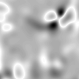
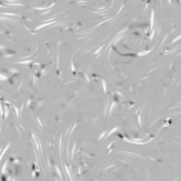
Figure 4: Snapshot of energy (left) and enstrophy (right) fluxes from the same vorticity field. Energy flux (3) is computed at scale $r_{1}=0.025L$ and enstrophy flux at $r_{2}=0.0025L$, roughly corresponding to the minimum and maximum in Fig. 3. White and black correspond to positive and negative values respectively.

Figure 4 shows that both positive and negative fluxes are observed: locally both energy and enstrophy can go to smaller or larger scales. Figure 5 shows the probability density functions of the two fluxes. As observed in previous studies CEEWX03 ; CEERWX06 , the shapes of pdf’s are nearly symmetric, confirming the qualitative picture inferred from Fig. 4. The mean values in both cases is the result of strong cancellations as its ratio with the standard deviation is $-0.22$ for the energy flux and $0.16$ for the enstrophy flux. The skewness is also small as it is about $0.9$ and $1.2$ for the energy and enstrophy fluxes respectively.

Figure 5: Probability density function of energy $\Pi^{(e)}_{r_{1}}$ (left) and enstrophy $\Pi^{(e)}_{r_{2}}$ (right) fluxes normalized with their standard deviations. Resolution is $N=8192$, filtering scales are $r_{1}=0.025L$ and $r_{2}=0.0025L$.

Figure 6 shows the joint probability density function $p(\Pi^{(e)}_{r_{1}},\Pi^{(z)}_{r_{2}})$ for the same scales $r_{1}$ and $r_{2}$. This pdf is not far from the product of the marginal distributions shown in Fig. 5, a condition for independence. Indeed, the cross correlation among $\Pi^{(e)}_{r_{1}}$ and $\Pi^{(z)}_{r_{2}}$ is only $C(r_{1},r_{2})\simeq-0.15$. Of course, it is very different if we consider the correlation at the same scale, for which we find $C(r,r)\simeq 1$ despite the fact that one of the fluxes has zero mean. A possible interpretation of the observed small value of correlation is in favor of the classical picture of independence of the two cascades which is here obtained at a local level. Therefore, our result is, a posteriori, a support to many experimental and numerical studies in which, due to finite size constraints, only one cascade is realized.

Figure 6: Joint probability density function $p(\Pi^{(e)}_{r_{1}},\Pi^{(z)}_{r_{2}})$ of energy (x-axis) and enstrophy (y-axis) fluxes. Scales $r_{1}$ and $r_{2}$ as in Fig. 5. Contours are plotted on a logarithmic scale while fluxes are normalized with their standard deviations.

In conclusion, we have presented statistical analysis of high resolution direct numerical simulations of 2D Navier-Stokes equations which clearly reproduce, for the first time, the double cascade scenario predicted by Kraichnan almost $40$ years ago.

- (1) R.H. Kraichnan, Inertial Ranges in Two-Dimensional Turbulence Phys. Fluids 10, 1417, (1967).
- (2) R.H. Kraichnan, Inertial-range transfer in two- and three-dimensional turbulence J. Fluid Mech. 47, 525, (1971).
- (3) R.H. Kraichnan and D. Montgomery, Two-dimensional turbulence Rep. Prog. Phys., 43, 547, (1980).
- (4) P. Tabeling, Two-dimensional turbulence: a physicist approach Phys. Rep. 362, 1, (2002).
- (5) D. Bernard, G. Boffetta, A. Celani and G. Falkovich, Conformal invariance in two-dimensional turbulence Nature Phys. 2, 124, (2006).
- (6) J. Paret and P. Tabeling, Experimental Observation of the Two-Dimensional Inverse Energy Cascade Phys. Rev. Lett. 79, 4162, (1997).
- (7) E. Siggia and H. Aref, Point-vortex simulation of the inverse energy cascade in two-dimensional turbulence Phys. Fluids 24, 171, (1981).
- (8) U. Frisch and P.L. Sulem, Numerical simulation of the inverse cascade in two-dimensional turbulence Phys. Fluids 27, 1921, (1984).
- (9) L. Smith and V. Yakhot, Bose condensation and small-scale structure generation in a random force driven 2D turbulence Phys. Rev. Lett. 71, 352, (1993).
- (10) G. Boffetta, A. Celani and M. Vergassola, Inverse energy cascade in two-dimensional turbulence: Deviations from Gaussian behavior Phys. Rev. E 61, R29 (2000).
- (11) B. Legras, P. Santangelo and R. Benzi, High-Resolution Numerical Experiments for Forced Two-Dimensional Turbulence Europhys. Lett. 5, 37 (1988).
- (12) H. Kellay, X.L. Wu and W.I. Goldburg, Experiments with Turbulent Soap Films Phys. Rev. Lett. 74, 3975 (1995).
- (13) V. Burue, Spectral exponents of enstrophy cascade in stationary two-dimensional homogeneous turbulence Phys. Rev. Lett. 71, 3967 (1993).
- (14) T. Gotoh, Energy spectrum in the inertial and dissipation ranges of two-dimensional steady turbulence Phys. Rev. E 57, 2984 (1998).
- (15) E. Lindborg and K. Alvelius, The kinetic energy spectrum of the two-dimensional enstrophy turbulence cascade Phys. Fluids 12, 945 (2000).
- (16) C. Pasquero and G. Falkovich, Stationary spectrum of vorticity cascade in two-dimensional turbulence Phys. Rev. E 65, 056305 (2002).
- (17) K. Nam, E. Ott, T.M. Antonsen and P.N. Guzdar, Lagrangian Chaos and the Effect of Drag on the Enstrophy Cascade in Two-Dimensional Turbulence Phys. Rev. Lett. 84, 5134 (2000).
- (18) G. Boffetta, A. Celani, S. Musacchio and M. Vergassola, Intermittency in two-dimensional Ekman-Navier-Stokes turbulence Phys. Rev. E 66, 026304 (2002).
- (19) M.A. Rutgers, Forced 2D Turbulence: Experimental Evidence of Simultaneous Inverse Energy and Forward Enstrophy Cascades Phys. Rev. Lett. 81, 2244 (1998).
- (20) C.H. Bruneau and H. Kellay, Experiments and direct numerical simulations of two-dimensional turbulence Phys. Rev. E 71, 046305 (2005).
- (21) S. Chen, R.E. Ecke, G.L. Eyink, X. Wang and Z. Xiao, Physical Mechanism of the Two-Dimensional Enstrophy Cascade Phys. Rev. Lett. 91, 214501 (2003).
- (22) S. Chen, R.E. Ecke, G.L. Eyink, M. Rivera, M. Wan and Z. Xiao, Physical Mechanism of the Two-Dimensional Inverse Energy Cascade Phys. Rev. Lett. 96, 084502 (2006).