Statistical Properties of Nonlinear Shell Models of Turbulence from Linear Advection Models: Rigorous Results

Abstract

In a recent paper it was proposed that for some nonlinear shell models of turbulence one can construct a linear advection model for an auxiliary field such that the scaling exponents of all the structure functions of the linear and nonlinear fields coincide. The argument depended on an assumption of continuity of the solutions as a function of a parameter. The aim of this paper is to provide a rigorous proof for the validity of the assumption. In addition we clarify here when the swap of a nonlinear model by a linear one will not work,

I Introduction

Shell models of turbulence GioBook ; bif03 serve a useful purpose in studying the statistical properties of turbulent fields due to their relative ease of simulation. In particular, shell models allowed accurate direct numerical calculation of the scaling exponents of their associated structure functions, including convincing evidence for their universality Gledzer ; GOY ; Jensen91PRA ; Piss93PFA ; Gat95PRE ; sabra . In contrast, for the Navier-Stokes equations that model actual fluid turbulence simulations are very much harder, and in addition one still does not know whether these equations in 3-dimensions are mathematically globally well posed. This problem does not exist in shell models 06CLT , adding to their numerical attractiveness a possibility to prove various properties and results rigorously 06CLT ; 06CLT_2 .

Consider for example the Sabra shell model sabra which, like other shell models of turbulence, is a truncated description of the dynamics of Fourier modes, preserving some of the structure and conservation laws of the Navier-Stokes equations:

$$(\frac{d}{dt} + \nu k_{n}^{2})u_{n}=i\big{[}k_{n+1}u_{n+1}^{*}u_{n+2}-\delta k_{n}u_{n-1}^{*}u_{n+1}$$ (1)

$$+ (1-\delta)k_{n-1}u_{n-1}u_{n-2}\big{]}+f_{n}\ .$$

Here $u_{n}$, with $n=0,1,2,\dots$ and the boundary conditions $u_{-2}=u_{-1}=0$, are the velocity modes restricted to ‘wavevectors’ $k_{n}=k_{0}\mu^{n}$ with $k_{0}$ determined by the inverse outer scale of turbulence. The model contains one additional parameter, $\delta$, and it conserves two quadratic invariants (when the force and the dissipation term are absent) for all values of $\delta$. The first is the total energy $\sum_{n}|u_{n}|^{2}$ and the second is $\sum_{n}(-1)^{n}k_{n}^{\alpha}|u_{n}|^{2}$, where $\alpha=\log_{\mu}(1-\delta)$.

The scaling exponents are properties of the structure functions. To define the structure function we introduce an average over time according to

$$\langle A(t)\rangle\equiv\lim_{T\to\infty}\frac{1}{T}\int_{0}^{T}A(t)dt\ .$$ (2)

In practice, however, we take

$$\langle A(t)\rangle=\frac{1}{T}\int_{0}^{T}A(t)dt\ ,$$ (3)

for some $T$ large enough, but finite. Our rigorous results also refer to this definition of an average over time. For values of the viscosity $\nu$ small enough, and for a sufficiently large amplitude of the random force $f_{n}$ there exists a large range of values $k_{n}$ where numerical simulations show that structure functions follow a power-law behavior. The low-order structure functions and the associated scaling exponents are

$$S_{2}(k_{n})\equiv\langle u_{n}u^{*}_{n}\rangle\sim k_{n}^{-\zeta_{2}}\ ,$$ (4)

$$S_{3}(k_{n})\equiv\Im\langle u_{n-1}u_{n}u_{n+1}^{*}\rangle\sim k_{n}^{-\zeta_{3}}\ ,$$ (5)

$$\text{etc. for higher order}~{}S_{p}(k_{n})\sim k_{n}^{-\zeta_{p}}\ .$$

The values of the scaling exponents were determined accurately by direct numerical simulations. Besides $\zeta_{3}$ which is exactly unity Piss93PFA , all the other exponents $\zeta_{p}$ appear anomalous, differing from $p/3$. Numerical evidence is that the scaling exponents are also universal, i.e. they are independent of the forcing $f_{n}$ as long as the latter is restricted to small $n$ bif03 . It was shown that for $0<\delta<1$ the leading scaling exponents are determined by the cascade of the energy invariant from large to small scales. For $1<\delta<2$ the second invariant $\sum_{n}(-1)^{n}k_{n}^{\alpha}|u_{n}|^{2}$ becomes important in determining the leading scaling exponents of the structure functions of $u_{n}$. In the bulk of this paper we consider the situation with $0<\delta<1$, but return to the other case in Sect. IV, in order to clarify the role of invariants in determining the scaling properties.

In a recent publication further insight to the anomaly of the exponents of the nonlinear problem (for the field $u_{n}$) was sought by relating them to the scaling exponents of a linear model for a field $w_{n}$. The linear model was constructed such that its scaling exponents should be the same as those of the nonlinear problem. The equations for this field are constructed under the following requirements: (i) the structure of the equations is obtained by linearizing the nonlinear problem and retaining only such terms that conserve the energy; (ii) the resulting equation is identical with the sabra model when $w_{n}=u_{n}$; (iii) the energy is the only quadratic invariant for the passive field in the absence of forcing and dissipation. These requirements lead to the following linear model:

$$\frac{dw_{n}}{dt}=\frac{i}{3}\Phi_{n}({\bm{u}},{\bm{w}})-\nu k_{n}^{2}w_{n}+f_{n}\ ,$$ (6)

where the advection term is defined as

$$\Phi_{n}({\bm{u}},{\bm{w}})=k_{n+1}[(1+\delta)u_{n+2}w_{n+1}^{*}+(2-\delta)u_{n+1}^{*}w_{n+2}]$$

$$+k_{n}[(1-2\delta)u_{n-1}^{*}w_{n+1}-(1+\delta)u_{n+1}w_{n-1}^{*}]$$

$$+k_{n-1}[(2-\delta)u_{n-1}w_{n-2}+(1-2\delta)u_{n-2}w_{n-1}]\ ,$$ (7)

together with $u_{-1}=u_{-2}=w_{-1}=w_{-2}=0$. Observe that when $w_{n}=u_{n}$ this model reproduces the Sabra model, and also that the total energy is conserved because $\sum_{n}\Im[\Phi_{n}(u,w)w^{*}_{n}]=0$. The second quadratic invariant is not conserved by the linear model (6). Finally, both models have the same ‘phase symmetry’ in the sense that the phase transformations $u_{n}\to u_{n}\exp{(i\phi_{n})}$ and $w_{n}\to w_{n}\exp{(i\theta_{n})}$ leave the equations invariant iff $\phi_{n-1}+\phi_{n}=\phi_{n+1}$, $\theta_{n-1}+\theta_{n}=\theta_{n+1}$. This identical phase relationship guarantees that the non-vanishing correlation functions of both models have precisely the same forms. Thus for example the only second and third correlation functions in both models are those written explicitly in Eqs. (4) and (5).

The advantage of the linear model is that correlation functions are advanced in time by a linear propagator 01ABCPM ; 02CGP ; fgv . The linear model possesses “Statistically Preserved Structures” (SPS) which are evident in the decaying problem Eq. (6) with $f_{n}=0$. These are left eigenfunctions of eigenvalue 1 of the linear propagators for each order (decaying) correlation function fgv . For example for the second order correlation function denote the propagator $P^{(2)}_{n,n^{\prime}}(t|t_{0})$; this operator propagates any initial condition $\langle w_{n}w^{*}_{n}\rangle(t_{0})$ (with average over initial conditions, independent of the realizations of the advecting field $u_{n}$) to the decaying correlation function (with average over realizations of the advecting field $u_{n}$)

$$\langle w_{n}w^{*}_{n}\rangle(t)=P^{(2)}_{n,n^{\prime}}(t|t_{0})\langle w_{n^{\prime}}w^{*}_{n^{\prime}}\rangle(t_{0})\ .$$ (8)

The second order SPS, $Z^{(2)}_{n}$, is the left eigenfunction with eigenvalue 1,

$$Z^{(2)}_{n^{\prime}}=Z^{(2)}_{n}P^{(2)}_{n,n^{\prime}}(t|t_{0})\ .$$ (9)

Note that $Z^{(2)}_{n}$ is time independent even though the operator $P^{(2)}_{n,n^{\prime}}(t|t_{0})$ is time dependent. Each order correlation function is associated with another propagator ${\bm{P}}^{(p)}(t|t_{0})$ and each of those has an SPS, i.e. a left eigenfunction ${\bm{Z}}^{(p)}$ of eigenvalue 1. These non-decaying eigenfunctions scale with $k_{n}$, ${\bm{Z}}^{(p)}\sim k_{n}^{-\xi_{p}}$, and the values of the exponents $\xi_{p}$ are anomalous. Finally, it was shown that these SPS are also the leading scaling contributions to the structure functions of the forced problem (6) fgv ; 01ABCPM . Thus the scaling exponents of the linear problem are independent of the forcing $f_{n}$, since they are determined by the SPS of the decaying problem.

To connect the linear model to the nonlinear problem one considers the system of two coupled equations

$$\frac{du_{n}}{dt} = \frac{i}{3}\Phi_{n}(u,u)+\frac{i\lambda}{3}\Phi_{n}(w,u)-\nu k_{n}^{2}u_{n}+f_{n}\ ,$$

$$\frac{dw_{n}}{dt} = \frac{i}{3}\Phi_{n}(u,w)+\frac{i\lambda}{3}\Phi_{n}(w,w)-\nu k_{n}^{2}w_{n}+\tilde{f}_{n}$$ (10)

with $\lambda$ being a real parameter and $f_{n}$ and $\tilde{f}_{n}$ being different realizations of the same random force. Observe that for any $\lambda\neq 0$, the two equations in (10) exchange roles under the change $\lambda w_{n}\leftrightarrow u_{n}$. Thus if the scaling exponents $\xi_{p}$ and $\zeta_{p}$ of the two fields exist (i.e. a true scaling range exists), they must be the same for all $\lambda\neq 0$. For $\lambda=0$ we recover the equations for the nonlinear and the linear models, Eqs. (1) and (6). In linnonlin it was assumed that the scaling exponents of either field exhibits no jump in the limit $\lambda\to 0$. Indeed, Ref. linnonlin also presented strong evidence for the validity of this assumption (see Fig. 1), but no mathematical proof was provided.

Figure 1: The sixth order structure function of the field $w_{n}$ in Eqs. (10) for $\lambda=10^{-1},10^{-3}$ and $10^{-5}$, together with the sixth order structure function for the Sabra model (1) and for the linear model (6), respectively. The structure function of the field $u_{n}$ for $\lambda>0$ are not shown since they are indistinguishable from those of the $w_{n}$. Inset: log-log plot of the fourth-order correlation function $F_{2,2}(k_{n},k_{7})$ vs. $k_{n}$ calculated for the linear field ($+$) and for the nonlinear field (solid line) at $\lambda=0$.

The aim of this paper is to close this gap. The main result of our paper states that the solutions of the system (10) exist globally in time and depend continuously on the parameter $\lambda$, including the limit $\lambda\to 0$. In particular we will show that if the structure function of $u_{n}$ and $w_{n}$ exhibit the same scaling exponents for any $\lambda\neq 0$, they will also have the same scaling exponents in the limit $\lambda\to 0$ (including $\lambda=0$). We would like to stress here that our rigorous results are valid for the structure functions, calculated over large, but finite, fixed interval of time, which is consistent with the definition (3) of the long time average. In addition, we would like to note that the numerical results correspond to the equations with the stochastic implementation of the forcing, while our rigorous proofs deal with the deterministic force that depend on time. The statement and the proof of the main theorem will be given in Section III. The proof is based on the results on the global existence and uniqueness of solutions of Eq. (1), obtained previously in 06CLT . In the following section we present the necessary mathematical definitions and formulate the essential statement from 06CLT .

II Functional Setting and Previous Analytic Results

II.1 Functional Setting

Following the classical treatment of the Navier-Stokes and Euler equations we re-write the sabra shell model for an infinite vector ${\bm{u}}\equiv(u_{0},u_{1},\dots)$

$$\frac{d{\bm{u}}}{dt}+\nu{\bm{A}}{\bm{u}}+\frac{i}{3}{\bm{\Phi}}({\bm{u}},{\bm{u}})={\bm{f}}\ ,$$ (11)

together with the initial conditions ${\bm{u}}(t=0)$. Introduce a Hilbert space $H$ which is the space of infinite vectors equipped with the scalar product $(\cdot,\cdot)$ and the corresponding norm $|{\cdot}|$ defined as

$$({\bm{u}},{\bm{v}})=\sum_{n=0}^{\infty}u_{n}v_{n}^{*},\quad|{\bm{u}}|=\bigg{(}\sum_{n=0}^{\infty}|u_{n}|^{2}\bigg{)}^{1/2},$$ (12)

for every ${\bm{u}},{\bm{v}}\in H$. The space $H$ is a space of all the velocity vectors having finite energy.

The linear operator ${\bm{A}}$, with a domain $D({\bm{A}})$ dense in $H$, is a positive definite, diagonal operator defined through its action on the elements ${\bm{u}}$ by

$${\bm{A}}{\bm{u}}=(k_{0}^{2}u_{0},k_{1}^{2}u_{1},\dots)$$ (13)

where the eigenvalues $k_{n}^{2}$ satisfy $k_{n}=k_{0}\mu^{n}$. Using the fact that ${\bm{A}}$ is a positive definite operator, we can define the powers ${\bm{A}}^{s}$ of ${\bm{A}}$ for every $s\in{\mathcal{R}}$

$$\forall{\bm{u}}=(u_{0},u_{1},u_{2},\dots),\quad{\bm{A}}^{s}u=(k_{0}^{2s}u_{0},k_{1}^{2s}u_{1},k_{2}^{2s}u_{2},\dots).$$ (14)

The space $D({\bm{A}}^{s/2})$ is the domain of the operator ${\bm{A}}^{s/2}$ and we denote

$$V_{s}\equiv D({\bm{A}}^{s/2})=\{{\bm{u}}=(u_{0},u_{1},u_{2},\dots)\ ,\sum_{j=0}^{\infty}k_{j}^{2s}|u_{j}|^{2}<\infty\},$$ (15)

which are Hilbert spaces equipped with the scalar product

$$({\bm{u}},{\bm{v}})_{s}=({\bm{A}}^{s/2}{\bm{u}},{\bm{A}}^{s/2}{\bm{v}}),\;\;\;\forall{\bm{u}},{\bm{v}}\in D({\bm{A}}^{s/2}),$$ (16)

and the norm $|{\bm{u}}|_{s}^{2}=({\bm{u}},{\bm{u}})_{s}$, for every ${\bm{u}}\in D({\bm{A}}^{s/2})$. Since $V_{s}$ contains velocity vectors with $s$ “derivatives”,

$$V_{s}\subseteq V_{0}=H\subseteq V_{-s},\;\;\;\forall s>0.$$ (17)

The case of $s=1$ is of a special interest for us. We denote $V=D({\bm{A}}^{1/2})$ a Hilbert space equipped with a scalar product and a corresponding norm

$$(({\bm{u}},{\bm{v}}))=({\bm{A}}^{1/2}{\bm{u}},{\bm{A}}^{1/2}{\bm{v}}),\;\;\;||{\bm{u}}||^{2}=(({\bm{u}},{\bm{u}})),$$ (18)

for every ${\bm{u}},{\bm{v}}\in V$. In addition the following relation holds

$$k_{1}|{\bm{u}}|\leq||{\bm{u}}||\ .$$ (19)

In what follows we will need the interpolation inequality for the spaces $V_{s}$.

Lemma 1. Let $s>0$, then for all ${\bm{u}}\in V_{s}$ and $0<s^{\prime}<s$

$$|{\bm{u}}|_{s^{\prime}}\leq|{\bm{u}}|^{1-s^{\prime}/s}|{\bm{u}}|_{s}^{s^{\prime}/s}\ .$$ (20)

Proof. The Lemma follows by a simple application of Hölder inequality.  

The bilinear operator $\frac{i}{3}{\bm{\Phi}}({\bm{u}},{\bm{w}})$ is defined above, cf. Eq. (7) together with ${\bm{\Phi}}\equiv(\Phi_{0},\Phi_{1},\dots)$. In 06CLT it was shown that such a definition of the bilinear operator makes ${\bm{\Phi}}$ and element of $H$ whenever ${\bm{u}}\in H$ and ${\bm{w}}\in V$. For any ${\bm{u}},{\bm{v}}\in H$ and ${\bm{w}}\in V$ one proves 06CLT

$$|({\bm{\Phi}}({\bm{u}},{\bm{v}}),{\bm{w}})|\leq C|{\bm{u}}|~{}|{\bm{v}}|~{}||{\bm{w}}||\ .$$ (21)

for some positive constant $C$. In addition the conservation law is written is the present notation as

$$\Im({\bm{\Phi}}({\bm{u}},{\bm{w}}),{\bm{w}})=0\ .$$ (22)

All our rigorous results are valid for the deterministic forcing ${\bm{f}}$. Therefore, in order to account for the stochastic implementation of the forcing term we will assume that ${\bm{f}}$ depends on time, but always stays bounded in the $H$-norm. More precisely, define the space $L^{\infty}([0,T),H)$, for some $0<T\leq\infty$, as a space of functions of the time interval $[0,T)$ with values in $H$ and the norm defined as

$$||{\bm{f}}||_{\infty}=\sup_{0\leq t<T}|{\bm{f}}(t)|\ .$$ (23)

In what follows, we will assume that the forcing term ${\bm{f}}$ satisfies ${\bm{f}}\in L^{\infty}([0,\infty),H)$.

II.2 Summary of Previous Results

In 06CLT Eq. (1) was studied, and the relevant results can be formulated as the following theorem:

Theorem (CLT 06): The solution of Eq. (1) exists globally in time for any initial condition ${\bm{u}}(0)$ in H, and for any ${\bm{f}}$ in $L^{\infty}([0,\infty),H)$. Moreover, the solutions are unique and the energy of the solution ${\bm{u}}(t)$ is bounded for all times:

$$\sup_{0\leq t\leq T}|{\bm{u}}(t)|^{2}\leq K_{0}(k_{0},\mu,\nu,\delta,{\bm{u}}(0),{\bm{f}})\ ,$$ (24)

where the a-priori constant $K_{0}$ depends on all the parameters of the equations, on the forcing and on the initial conditions.

If in addition we assume that the forcing ${\bm{f}}=(f_{0},f_{1},\dots)$ acts on the finite number of shells, namely, if there exists $N\geq 0$, such that $f_{n}=0$, for all $n\geq N$, then the solution ${\bm{u}}=(u_{0},u_{1},\dots)$ has an exponentially decaying spectrum $|u_{n}|$ as a function of $k_{n}$, and in particular

$$\sup_{\nu k_{0}^{2}\leq t\leq T}|{\bm{u}}(t)|_{s}^{2}\leq K_{s}(k_{0},\mu,\nu,\delta,{\bm{u}}(0),{\bm{f}}),$$ (25)

for any $s>0$ and the a-priori constants $K_{s}$ depend on all the parameters of the equations, on the forcing and on the $L^{\infty}([0,\infty),H)$-norm of the initial conditions (see definition (23)).

III The Main Result

The main statement of this paper is that the system of equations (10) is globally well posed for all real $\lambda$, and that the solutions depend continuously on the parameter $\lambda$. In particular, as $\lambda\to 0$ the solution of the system converge uniformly on any finite interval of time to the solution of the system with $\lambda=0$. This statement is formulated as follows:

Theorem 1. Let ${\bm{u}}(0;\lambda),{\bm{w}}(0;\lambda)$ be given in $H$, and the forces ${\bm{f}},{\bm{\tilde{f}}}$ in $L^{\infty}([0,T],H)$. Denote by ${\bm{u}}(t;\lambda),{\bm{w}}(t;\lambda)$ the solutions of the coupled system (10). Then the following holds

1. The solution of the system (10) exists globally in time for every $\lambda$. Moreover, energy of the solutions $|{\bm{u}}(t;\lambda)|^{2}$ and $|{\bm{w}}(t;\lambda)|^{2}$ are bounded for all times, where the bounds depend on all the parameters of the equations, $\lambda$, the forcing and the initial conditions.

2. For any $T>0$,

   $$\lim_{\lambda\to 0}\sup_{0\leq t\leq T}|{\bm{u}}(t;\lambda)-{\bm{u}}(t;0)|^{2}=0,$$

   and

   $$\lim_{\lambda\to 0}\sup_{0\leq t\leq T}|{\bm{w}}(t;\lambda)-{\bm{w}}(t;0)|^{2}=0,$$

   where ${\bm{u}}(t;0),w(t;0)$ are the solutions of (10) with $\lambda=0$.

3. If in addition we assume that the forces $f,{\tilde{f}}$ act only on the finite number of shells then for any $T\geq\nu k_{0}^{2}$, and $s>0$,

   $$\lim_{\lambda\to 0}\sup_{\nu k_{0}^{2}\leq t\leq T}|{\bm{u}}(t;\lambda)-{\bm{u}}(t;0)|_{s}^{2}=0,$$

   and

   $$\lim_{\lambda\to 0}\sup_{\nu k_{0}^{2}\leq t\leq T}|{\bm{w}}(t;\lambda)-{\bm{w}}(t;0)|_{s}^{2}=0,$$

   where ${\bm{u}}(t;0),w(t;0)$ are the solutions of (10) with $\lambda=0$.

Proof: Part 1. of this theorem follows from defining a new variable ${\bm{q}}(t;\lambda)\equiv{\bm{u}}(t;\lambda)+\lambda{\bm{w}}(t;\lambda)$. This variable satisfies Eq. (1) with a forcing ${\bm{f}}+\lambda{\bm{\tilde{f}}}$. Accordingly theorem CLT06 provides the proof that ${\bm{q}}(t;\lambda)$ exists globally in time for every $\lambda$. Next observe that the system of equations (10) can be rewritten in the form

$$\frac{du_{n}}{dt} = \frac{i}{3}\Phi_{n}({\bm{q}},{\bm{u}}))-\nu k_{n}^{2}u_{n}+f_{n}\ ,$$

$$\frac{dw_{n}}{dt} = \frac{i}{3}\Phi_{n}({\bm{q}},{\bm{w}})-\nu k_{n}^{2}w_{n}+\tilde{f}_{n}\ .$$ (26)

This form of writing shows that the the fields ${\bm{u}}$ and ${\bm{w}}$ satisfy linear diffusion advection equations advected by a smooth field ${\bm{q}}$. Accordingly both fields remain smooth for all time and all $\lambda$. In addition, using the relation (24) one is able to derive the bounds for the energies of the solutions.

To prove Part 2. of the theorem we need first
Proposition 1: Denote by ${\bm{q}}(t;0)$ the solution of the Sabra model (1) with initial data ${\bm{q}}(0;0)$ in $H$. That is also the solution of the first of equations (10) when $\lambda=0$. Then

$$\lim_{\lambda\to 0}\sup_{0\leq t\leq T}|{\bm{q}}(t;\lambda)-{\bm{q}}(t;0)|=0.$$

Moreover, if ${\bm{f}},$ and $\tilde{{\bm{f}}}$ act only on finite number of shells, then for any $s>0$ we have

$$\lim_{\lambda\to 0}\sup_{\nu k_{0}^{2}\leq t\leq T}|{\bm{q}}(t;\lambda)-{\bm{q}}(t;0)|_{s}=0.$$

Proof: Let us denote by $\Delta{\bm{q}}={\bm{q}}(t;\lambda)-{\bm{q}}(t;0)$. Then $\Delta{\bm{q}}$ satisfies the equation

$$\frac{d\Delta{\bm{q}}}{dt}+\nu{\bm{A}}\Delta{\bm{q}}-\frac{i}{3}{\bm{\Phi}}({\bm{q}}(t;\lambda),\Delta{\bm{q}})-\frac{i}{3}{\bm{\Phi}}(\Delta{\bm{q}},{\bm{q}}(t;\lambda))$$

$$+\frac{i}{3}{\bm{\Phi}}(\Delta{\bm{q}},\Delta{\bm{q}})=\lambda{\bm{\tilde{f}}}$$ (27)

$$\Delta{\bm{q}}(0)=\lambda{\bm{w}}(0).$$ (28)

Take now the inner product in $H$ of the above equation with $\Delta{\bm{q}}$. Computing the real part and using Eq. (22) we find

$$\frac{1}{2}\frac{d}{dt}|\Delta{\bm{q}}|^{2}+\nu||\Delta{\bm{q}}||^{2}-\Re(\frac{i}{3}{\bm{\Phi}}(\Delta{\bm{q}},{\bm{q}}(t;\lambda),\Delta{\bm{q}})=\Re(\lambda{\bm{\tilde{f}}},\Delta{\bm{q}})\ .$$ (29)

Using the Cauchy-Schwarz inequality and the relation (21) we get

$$\frac{1}{2}\frac{d}{dt}|\Delta{\bm{q}}|^{2}+\nu||\Delta{\bm{q}}||^{2}\leq$$

$$\leq|(\frac{1}{3}{\bm{\Phi}}(\Delta{\bm{q}},{\bm{q}}(t;\lambda),\Delta{\bm{q}})|+|(\lambda\tilde{f},\Delta{\bm{q}})|$$

$$\leq C|\Delta{\bm{q}}|~{}||\Delta{\bm{q}}||~{}|q(t;\lambda)|+\lambda|{\bm{\tilde{f}}}|~{}|\Delta{\bm{q}}|\ ,$$ (30)

Applying the Young’s inequality ($ab\leq a^{2}/2+b^{2}/2$) twice and using the inequality (19), we have

$$\frac{1}{2}\frac{d}{dt}|\Delta{\bm{q}}|^{2}+\nu||\Delta{\bm{q}}||^{2}\leq\frac{C^{2}}{\nu}|\Delta{\bm{q}}|^{2}|q(t;\lambda)|^{2}+\frac{\lambda^{2}}{\nu k_{1}^{2}}|{\bm{\tilde{f}}}|^{2}+\frac{\nu}{2}||\Delta{\bm{q}}||^{2}.$$

Using the fact that the relation (24) holds for any $t\geq 0$ and the fact that ${\bm{f}}\in L^{\infty}([0,\infty),H)$ (see definition (23)), we obtain

$$\frac{d}{dt}|\Delta{\bm{q}}|^{2}\leq\frac{2K_{0}^{2}C^{2}}{\nu}|\Delta q|^{2}+\frac{2\lambda^{2}}{\nu k_{1}^{2}}||{\bm{\tilde{f}}}||_{\infty}^{2}.$$

By Gronwall’s inequality we conclude

$$|\Delta{\bm{q}}(t)|^{2}\leq$$

$$\leq e^{\frac{2K_{0}^{2}C^{2}}{\nu}t}|\Delta{\bm{q}}(0)|^{2}+\frac{\lambda^{2}||{\bm{\tilde{f}}}||_{\infty}^{2}}{K_{0}^{2}C^{2}k_{1}^{2}}(e^{\frac{2K_{0}^{2}C^{2}}{\nu}t}-1)=$$

$$=e^{\frac{2K_{0}^{2}C^{2}}{\nu}t}\lambda^{2}|{\bm{w}}(0)|^{2}+\frac{\lambda^{2}||{\bm{\tilde{f}}}||_{\infty}^{2}}{K_{0}^{2}C^{2}k_{1}^{2}}(e^{\frac{2K_{0}^{2}C^{2}}{\nu}t}-1).$$ (31)

Therefore, for any $T>0$,

$$\lim_{\lambda\to 0}\sup_{0\leq t\leq T}|\Delta{\bm{q}}(t)|^{2}=0,$$

and the first statement of the proposition follows.

The second statement of the proposition follows from the boundedness of ${\bm{q}}(t;\lambda)$ and ${\bm{q}}(t;0)$ in higher order norms after a short transient period of times, say $\nu k_{0}^{2}$, (provided that the forces ${\bm{f}},$ and $\tilde{{\bm{f}}}$ act on the finite number of shells as required by Theorem CLT06) and the interpolation inequality (20).  

Finally, we are ready to finish the proof of the main theorem. Let us fix $s\geq 0$, and show that

$$\lim_{\lambda\to 0}\sup_{\nu k_{0}^{2}\leq t\leq T}|{\bm{w}}(t;\lambda)-{\bm{w}}(t;0)|_{s}^{2}=0.$$ (32)

Denote $\Delta{\bm{w}}={\bm{w}}(t;\lambda)-{\bm{w}}(t;0)$. The function $\Delta{\bm{w}}$ satisfies the equation

$$\frac{d}{dt}\Delta{\bm{w}}+\nu{\bm{A}}\Delta{\bm{w}}-\frac{i}{3}{\bm{\Phi}}\big{(}{\bm{q}}(t;\lambda),{\bm{w}}(t;\lambda)\big{)}$$

$$+\frac{i}{3}{\bm{\Phi}}\big{(}{\bm{q}}(t;0),{\bm{w}}(t;0)\big{)}=0.$$ (33)

We rewrite it in the form

$$\frac{d}{dt}\Delta{\bm{w}}+\nu{\bm{A}}\Delta{\bm{w}}-\frac{i}{3}{\bm{\Phi}}\big{(}{\bm{q}}(t;\lambda)-{\bm{q}}(t;0),{\bm{w}}(t;0)\big{)}-\frac{i}{3}{\bm{\Phi}}\big{(}{\bm{q}}(t;\lambda),\Delta{\bm{w}}\big{)}=0,$$ (34)

and as before, taking the inner product in $H$ with $\Delta{\bm{w}}$, computing the real part and using Eq. (22), we obtain

$$\frac{1}{2}\frac{d}{dt}|\Delta{\bm{w}}|^{2}+\nu||\Delta{\bm{w}}||^{2}-\Re\Big{(}\frac{i}{3}{\bm{\Phi}}\big{(}{\bm{q}}(t;\lambda)-{\bm{q}}(t;0),{\bm{w}}(t;0)\big{)},\Delta{\bm{w}}\Big{)}=0.$$

Applying, subsequently the Young’s inequality and the inequality (21), we get

$$\frac{1}{2}\frac{d}{dt}|\Delta{\bm{w}}|^{2}+\nu||\Delta{\bm{w}}||^{2}\leq|\big{(}\frac{i}{3}{\bm{\Phi}}\big{(}{\bm{q}}(t;\lambda)-{\bm{q}}(t;0),{\bm{w}}(t;0)\big{)},\Delta{\bm{w}}\big{)}|\leq$$

$$\leq C||\Delta{\bm{w}}||~{}|{\bm{w}}(t;0)|~{}|{\bm{q}}(t;\lambda)-{\bm{q}}(t;0)|\leq\frac{C^{2}}{2\nu}|{\bm{w}}(t;0)|^{2}~{}|{\bm{q}}(t;\lambda)-{\bm{q}}(t;0)|^{2}+\frac{\nu}{2}||\Delta{\bm{w}}||^{2}.$$ (35)

It follows that

$$\frac{d}{dt}|\Delta{\bm{w}}|^{2}\leq\frac{C^{2}}{\nu}|{\bm{w}}(t;0)|^{2}|{\bm{q}}(t;\lambda)-{\bm{q}}(t;0)|^{2},$$

and integrating over $(0,t)$ we conclude

$$|\Delta{\bm{w}}(t)|^{2}\leq\frac{C^{2}M}{\nu}t|{\bm{q}}(t;\lambda)-{\bm{q}}(t;0)|^{2},$$

where we used the fact that $\Delta{\bm{w}}(0)=0$ and $|{\bm{w}}(t;0)|^{2}\leq M$, for some constant $M$, as was stated in the Part 1 of the main theorem. It follows from Proposition 1 that $\sup_{0\leq t\leq T}|{\bm{q}}(t;\lambda)-q(t;0)|^{2}\to 0$, as $\lambda\to 0$. Hence we may conclude that

$$\lim_{\lambda\to 0}\sup_{0\leq t\leq T}|\Delta{\bm{w}}(t)|^{2}=0.$$

By virtue of the interpolation inequality (20) one can follow steps as in the proof of Proposition $1$ to show that the higher order norms of $\Delta{\bm{w}}$ also converge to $0$ uniformly in the time interval $\nu k_{0}^{2}\leq t\leq T$, as $\lambda\to 0$. To finish the proof, on can observe that

$$|{\bm{u}}(t;\lambda)-{\bm{u}}(t;0)|=|{\bm{q}}(t;\lambda)-{\bm{q}}(t;0)-\lambda{\bm{w}}(t;\lambda)|$$

$$\leq|{\bm{q}}(t;\lambda)-{\bm{q}}(t;0)|+\lambda|{\bm{w}}(t;\lambda)|,$$ (36)

and from the fact that $|{\bm{w}}(t;\lambda)|$ is globally bounded in time it follows from Proposition 1 that

$$\lim_{\lambda\to 0}\sup_{0\leq t\leq T}|{\bm{u}}(t;\lambda)-{\bm{u}}(t;0)|=0.$$

 

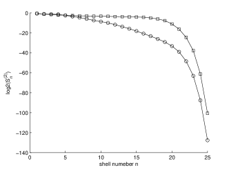
Figure 2: Double logarithmic plot of the second order structure functions $\langle u_{n}u^{*}_{n}\rangle$ and $\langle w_{n}w^{*}_{n}\rangle$ of the system of equations (10) for $\delta=1.25$ and $\lambda=0$.

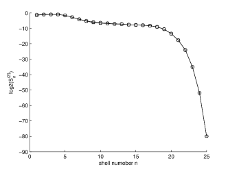
Figure 3: Double logarithmic plot of the second order structure functions $\langle u_{n}u^{*}_{n}\rangle$ and $\langle w_{n}w^{*}_{n}\rangle$ of the system of equations (10) for $\delta=1.25$ and $\lambda=1$.

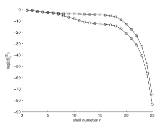
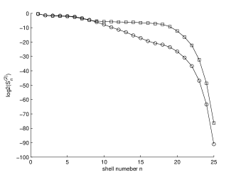
Figure 4: Double logarithmic plot of the second order structure functions $\langle u_{n}u^{*}_{n}\rangle$ and $\langle w_{n}w^{*}_{n}\rangle$ of the system of equations (10) for $\delta=1.25$ and $\lambda=0.1$ (upper panel) and $\lambda=0.01$ (lower panel).

III.1 Consequences for Structure Functions

Using the form of Eqs. (26) we conclude that for $f_{n}$ and $\tilde{f}_{n}$ being different realizations of the same random force, whenever the structure functions of $u_{n}$ and $w_{n}$ exhibit the same scaling exponents for all finite $\lambda$, they must also exhibit the same scaling exponents for $\lambda=0$.

IV When can the Nonlinear Model exhibit Scaling Exponents that are Different from the Linear Model

In this section we turn our attention to situations when the nonlinear and the linear models cannot exhibit the same scaling exponents. The theorem as stated and proven still holds, but as we shall see this is a situation for which the two fields $u_{n}$ and $w_{n}$ cannot exhibit the same scaling exponents for all $\lambda\neq 0$. A case in point is the same nonlinear Sabra model with $1<\delta<2$. In Fig. 2 we show the second order structure functions $\langle u_{n}u^{*}_{n}\rangle$ and $\langle w_{n}w^{*}_{n}\rangle$ obtained from simulating Eqs. (10) for $\lambda=0$ and $\delta=1.25$. As expected, the scaling of $w_{n}$ is influenced by the cascade of energy, whereas that of $u_{n}$ by the cascade of the second invariant. As a result the scaling exponents are distinctly different. The same system of equations for $\lambda=1$ is symmetric in $w_{n}$ and $u_{n}$. Indeed, in Fig. 3 we show the result of simulations for $\lambda=1$, for which the second order structure function of the two fields is identical. Now however we cannot expect that this identity will persist for $\lambda\to 0$. In Fig, 4 we show the results of simulations for the same system of equations for $\lambda=0.1$ and $\lambda=0.01$.

To understand the results of the simulations we note that when $\lambda\neq 0$ the second invariant of the equation for $u_{n}$ is destroyed, and one could think that the scaling of $u_{n}$ should be dominated by the energy invariant. This is certainly true for $\lambda=1$. But now when $\lambda$ decreases towards zero, we should reconsider the system of equations (10) by renaming $\tilde{w}_{n}=\lambda w_{n}$. Substituting this re-named variables into Eqs. (10) and re-arranging, we read

$$\frac{du_{n}}{dt} = \frac{i}{3}\Phi_{n}(u,u)+\frac{i}{3}\Phi_{n}(\tilde{w},u)-\nu k_{n}^{2}u_{n}+f_{n}\ ,$$

$$\frac{d\tilde{w}_{n}}{dt} = \frac{i}{3}\Phi_{n}(u,\tilde{w})+\frac{i}{3}\Phi_{n}(\tilde{w},\tilde{w})-\nu k_{n}^{2}\tilde{w}_{n}+\lambda\tilde{f}_{n}\ .$$ (37)

Thus the net result of the transformation is that the equations for $u_{n}$ and $\tilde{w}_{n}$ are the same, but the forcing of $w_{n}$ becomes weaker and weaker as $\lambda\to 0$. Accordingly, while the second invariant is still destroyed as a true invariant for any value of $\lambda$, for small $\lambda$ the strength of the term $\frac{i}{3}\Phi_{n}(\tilde{w},u)$ diminishes, allowing a cross-over behavior in the scaling of $u_{n}$, precisely as we see in Fig. 4.

- (1) T. Bohr, M.H. Jensen, G. Paladin, A. Vulpiani, Dynamical systems approach to turbulence (Cambridge University Press, 1998)
- (2) L. Biferale Ann. Rev. Fluid. Mech. 35, 441, (2003).
- (3) E. B. Gledzer. Dokl. Akad. Nauk. SSSR, 20, 1046 (1973).
- (4) M. Yamada and K. Ohkitani. J. Phys. Soc. Jpn 56, 4210 (1987).
- (5) M. H. Jensen, G. Paladin, and A. Vulpiani. Phys. Rev. A, 43, 798 (1991).
- (6) D. Pissarenko, L. Biferale, D. Courvoisier, U. Frisch, and M. Vergassola. Phys. Fluids A 5, 2533 (1993).
- (7) I. Procaccia O. Gat and R. Zeitak. Phys. Rev. E , 51, 1148 (1995).
- (8) V.S. L’vov, E. Podivilov, A. Pomyalov, I. Procaccia and D. Vandembroucq, Phys. Rev. E , 58 1811(1998).
- (9) R. Benzi, L. Biferale, and G. Parisi. Physica D 65, 163 (1993).
- (10) R. Benzi, L. Biferale and F. Toschi Eur. Phys. J. B 24, 125, (2001).
- (11) R. Benzi, L. Biferale, M. Sbragaglia and F. Toschi Phys. Rev. E 68, 046304, (2004).
- (12) P. Ditlevsen, Phys. Rev. E, 54 985, (1996).
- (13) L. Biferale, D. Pierotti and F. Toschi Phys. Rev. E 57, R2515, (1998).
- (14) G. Falkovich, K. Gawedzk, M. Vergassola, Rev. Mod. Phys. 73 913 (2001).
- (15) I. Arad, L. Biferale, A. Celani, I. Procaccia, and M. Vergassola, Phys. Rev. Lett., 87, 164502 (2001) .
- (16) Y. Cohen, T. Gilbert and I. Procaccia, Phys. Rev. E., 65,026314 (2002).
- (17) I. Arad and I. Procaccia, Phys. Rev. E, 63, 056302 (2001).
- (18) A. Celani and M. Vergassola, Phys. Rev. Lett., 86 424 (2001).
- (19) Y. Cohen, A. Pomyalov and I. Procaccia, Phys. Rev. E., 68, 036303 (2003).
- (20) L. Angheluta, R. Benzi, L. Biferale, I. Procaccia and F. Toschi, Phys. Rev. Lett., in press.
- (21) P. Constantin, B. Levant and E. S. Titi, Physica D 219 (2006), 120-141.
- (22) P. Constantin, B. Levant and E. S. Titi, Phys. Rev. E, accepted.