Nonperiodic echoes from mushroom billiard hats

Abstract

Mushroom billiards have the remarkable property to show one or more clear cut integrable islands in one or several chaotic seas, without any fractal boundaries. The islands correspond to orbits confined to the hats of the mushrooms, which they share with the chaotic orbits. It is thus interesting to ask how long a chaotic orbit will remain in the hat before returning to the stem. This question is equivalent to the inquiry about delay times for scattering from the hat of the mushroom into an opening where the stem should be. For fixed angular momentum we find that no more than three different delay times are possible. This induces striking nonperiodic structures in the delay times that may be of importance for mesoscopic devices and should be accessible to microwave experiments.

I Introduction

Two-dimensional billiards play a central role in the development of chaos theory ever since the early work of Sinai sinai . In physics they have acquired increasing importance as they are seen to emulate properties of systems as different as quantum dots qdots or planetary rings benet . Particularly quantum or wave realizations of such objects have become popular, since flat microwave cavities, so-called microwave billiards, are used by experimentalists at different laboratories smilansky ; stoeckmann ; richter ; sirko ; anlage ; sridhar ; legrand , and these experiments mimic some properties of mesoscopic devices. From a mathematical point of view one of the advantages of billiards is that, in many instances, chaotic properties can be proven for cases of complete chaos sinai ; bunimovich1 ; threedisk ; threehills and more recently even for mixed systems bunimovich2 ; jung .

Microwave billiards serve as an analog system for the experimental study of the wave behavior of the corresponding classical billiard, and permit a direct test of hypotheses proposed concerning connections between the quantum and the corresponding classical dynamic Stockmann ; IMAPRO . In particular the spectral behavior and properties of the wave functions of quantum systems, whose classical analogue is chaotic Casati ; Bohigas ; Berry ; Leyvraz ; Sieber ; Braun-Haake , integrable Gutzwiller ; Berry-Tabor or intermediate SVZ ; Berry-Robnik ; SV-JPA can be investigated experimentally with such systems. In scattering systems similar matters have been discussed mainly for systems that are chaotic and hyperbolic threedisk ; Jung-Dietz , or mixed Ketzmerick ; Jung-Seligman ; carlosnjp ; mejia ; friedrich . The role of parabolic manifolds has also received considerable attention richter ; Dietz-Lombardi .

Mixed systems typically have the property, that in some border region integrable and chaotic areas intermingle as a fractal. Such a scenario is well illustrated by the twist map twistmap . It may help to detect some characteristics of the dynamics in certain cases friedrich . Bunimovich bunimovich2 has proposed a family of mushroom billiards with mixed phase space which have the unusual property that chaotic areas and integrable ones are not separated by a fractal set of integrable islands extending into the chaotic sea. Such billiards are characterized by circular or elliptic hats connected to a stem or stems composed of straight walls; we shall concentrate on the case with only one hat and one stem. Typical examples are shown in Fig. 1. The stem pertains entirely to the chaotic area, while the hat houses both chaotic and integrable trajectories. Several studies on the classical dynamics in mushroom billiards have already been presented altmann ; mushroomworks .

It is clear, that the relevant properties of such a billiard are determined by the hat of the mushroom, and in view of the successful theoretical mejia and experimental friedrich analysis of phase space structures in the context of scattering echoes we wish in the present paper to analyze the hat of the mushroom alone, viewed as a scattering system with an opening where the stem used to be; yet to establish contact with other work, we shall also keep the possibility of a stem in mind. In the spirit of scattering echoes we ask how long a particle stays in the hat, if injected from the opening of the billiard or from the stem. Note that in the case of a semicircle mushroom hat with a symmetric stem, the limit of the area of stable bounded orbits is a caustic, which forms a circle segment connecting the points where the stem starts, as seen in the mushroom billiard in Fig. 1(a). The usual Smale horseshoe construction jung fails, because there is no hyperbolic periodic orbit along this line. We have therefore numerically investigated the distribution of the classical delay times of such a billiard and found a surprising selectivity in the allowed delay times.

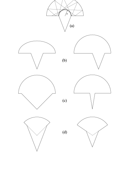
Figure 1: Different shapes of mushroom hats. Circular mushroom billiards consist of a hat with a circular boundary and a stem, which has been chosen in triangular form for all mushroom billiards here. Stable orbits in a circular mushroom hat never enter the stem. They form a caustic in the hat, and the radius of the smallest possible caustic is one-half the width of the stem, as indicated in (a). Other shapes of mushroom billiards may display an elliptic hat or a shifted stem (b), very wide or narrow stems (c) or hats which are a circle sector of an angle smaller than 180^∘ (d), in this case $90^{\circ}$ and $180^{\circ}\times(\sqrt{5}-1)/2$.

As the angular momentum is a constant of motion in the scattering process as long as a particle stays within the hat we shall first consider fixed angular momenta and we find that generically only three delay times occur. On a subset of measure zero, one and two delay times are also possible; a larger set of different delay times is outright forbidden. This result is intimately related to old results on the circle map slater and allows to understand the above mentioned selectivity.

II Definitions and preliminary results

The circular hats of mushrooms are characterized by two quantities: The position and size of the hole and the angle between the straight walls that constitute the underside of the hat. In Fig. 1 we show various hats of mushroom billiards with different properties: circular mushroom hats [(a) and (c)], mushroom billiards with a shifted stem or an elliptic hat (b) and mushroom billiards whose hat is a circle sector of an angle different from $180^{\circ}$ (d). The stem is always chosen in triangular form to avoid the trivial parabolic manifold of so-called ”bouncing ball” orbits between parallel walls of a rectangular stem.

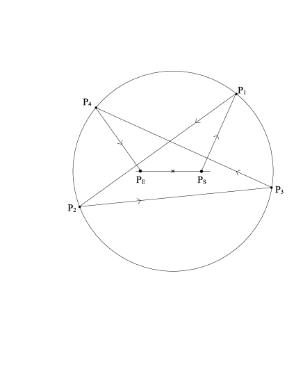
Figure 2: The $\Theta$ billiard is a circle billiard with a straight line of length $2r$ along a diameter of the circle of length $2R$, which defines the starting and ending points of the particle orbits taken into consideration. In a semicircle mushroom hat with the opening located at the position of the straight line these orbits correspond to those of particles entering and leaving it. In this sketch, a particle starts from the straight line at $P_{S}$, undergoes four reflections with the boundary at $P_{1}$, $P_{2}$, $P_{3}$, and $P_{4}$ before it finally ends on the straight line at $P_{E}$.

In Fig. 1(c) we show $180^{\circ}$-mushroom billiards with a wide and a narrow stem, respectively. Here a narrow stem is one narrow enough, that orbits which are triangular in the full circle remain within the hat irrespective of the orientation of the triangle. This implies, that all polygons, which do not form stars with intersecting line segments are confined to the hat. Moreover, the delay time, i.e., the time a particle entering the mushroom hat stays there, is approximately determined by the number of its bounces off the circle boundary. This is clearly not the case for a wide stem, where some polygons are no longer confined to the hat. In the following we will restrict ourselves to mushroom billiards with a narrow stem and count bounces of particles entering and leaving the mushroom hat, instead of determining delay times.

We also show mushroom billiards where the two straight walls constituting the underside of the hat have angles smaller than $180^{\circ}$ in Fig. 1(d). Note that it is essential that the two straight walls are parts of radii of the circle, i.e., form an angle of $90^{\circ}$ with the tangent to the circle boundary at their intersection. Otherwise we lose the properties of the mushroom billiard. If the angle is larger than $90^{\circ}$, such that the extensions of the two straight walls meet in a point below the center of the circle, the system becomes ergodic and chaotic bunimovich3 . For an angle smaller than $90^{\circ}$ we get a more complex coexistence of integrable and chaotic dynamics.

In the following we first will consider open $180^{\circ}$-mushroom billiards with a semicircular hat and a symmetric stem. We are interested in the number of bounces a particle entering a mushroom hat through the opening experiences at the circle boundary before exiting again. Bounces with the straight part of the boundary are not counted. Whenever the particle hits it, we may use the principle of mirror images princ , i.e., reflect the semicircle across its straight boundary, thereby obtaining a complete circle and continue the orbit into its lower half. Accordingly, we may introduce a convenient alternative system, the so-called $\Theta$ billiard altmann shown in Fig. 2, which consists of a circle billiard, whose radius $R$ equals that of the mushroom hat, and a straight line of length $2r$ where the opening of the corresponding semicircle mushroom hat is. The only purpose of the straight line is, that it defines the starting and the endpoints of those particle orbits we are interested in. In the mushroom billiard these correspond to particles entering and leaving the semicircle hat. Accordingly, in order to compute delay times, we consider particle orbits starting on the straight line in the $\Theta$ billiard and count the number of bounces of the particle with the circle boundary, until it again reaches the straight line. We shall see that the $\Theta$ billiard can be readily generalized to describe arbitrary mushroom hats. While the $\Theta$ billiard is convenient for mathematical purposes physically it seems of little direct use.

As already noted above and indicated in Fig. 1(a), for every particle orbit in the circle billiard the line segments connecting subsequent reflection points form a caustic of circular shape around the center of the billiard. The radius of the caustic equals the distance of these line segments from the circle center. Therefore it gives the angular momentum of the particle where we set the absolute value of the momentum to unity, as it is a conserved quantity. If the angular momentum of the particle is large enough, the corresponding orbit will never hit the straight line in the $\Theta$ billiard. Such orbits belong to the integrable part of the phase space of the mushroom billiard. If they are periodic they may be polygons or stars. If they are aperiodic they will correspond to slowly rotating stars or polygons, i.e., they would be periodic in some rotating frame of reference. The limiting angular momentum corresponds to the radius of that caustic, which just touches one or both ends of the straight line. Any aperiodic orbit with angular momentum smaller than the limiting value will eventually reach the straight line after some number of bounces. For periodic orbits we can have the particular case, where a star or polygon will intersect the straight line in certain orientations and not in others. The orientations that do not lead to intersections will yield a parabolic manifold in the chaotic sea as explained in Ref.  altmann . This paper focuses on orbits that do cross the straight line.

We now come to a really surprising result. Using a simple reflection program, which computes orbits of a particle in a billiard based on the law of specular reflection, we counted the bounces off the circle boundary a particle starting from the straight line with randomly chosen initial conditions experiences until it reaches the straight line again. We found a strange selectivity in these numbers, which resembled a generalized Fibonacci sequence. Indeed for $r=R/3$ the first observed numbers of bounces are 1, 4, 5, 9, 14, 23, 37. The next number in this sequence, 51, does not continue the Fibonacci series, but is the sum of 37 and 14. Similar results have been found for other ratios $r/R$. We shall call the possible numbers of bounces.

The purpose of this paper is to understand the observed selectivity. For this we will introduce a map, which generates the dynamics in the mushroom hat in an efficient way and then shall proceed in two steps utilizing this map. First we shall analyze the problem for a fixed angular momentum, considering that angular momentum is a conserved quantity both in the open mushroom hat and in the $\Theta$ billiard. We shall obtain the surprising result that typically only three magic numbers termed a magic triplet are possible for each angular momentum. To understand the entire delay time structure, we then analyze how these triplets evolve when changing the angular momentum. Based on the map, we developed a very efficient algorithm for the computation of the magic numbers.

III Magic numbers for fixed angular momentum

Let the radius of the $\Theta$ billiard be $R$ and the straight line of length $2r$ be oriented symmetrically along the horizontal axis. A particle orbit is characterized by the particle’s angular momentum $M$, which is just the radius of its caustic. Orbits with angular momentum $M>r$ never intersect the straight line, whereas orbits with $M<r$ intersect it (up to a set of marginally unstable orbits of measure zero as stated above) at some time and therefore correspond to chaotic trajectories in the mushroom billiard. The angular momentum can be expressed in terms of the angle between the orbit of the reflected particle and the tangent to the circle boundary at the point of impact, which also is a constant for each particle orbit; we will call this angle $\psi$, where $0<\psi\leq\pi/2$ (see Fig. 3). Then, the radius of the caustic, i.e., the angular momentum $M$ equals

$$M=R\cos\psi\,.$$ (1)

A particle orbit is also characterized by its initial orientation. Generally, the orientation of the particle orbit after $n$ reflections at the circle boundary may be given in terms of the orbit’s angle with the positive horizontal axis. Equivalently, its orientation may be defined in terms of the total angle covered by the vector pointing from the circle center to the point of contact between the caustic and the orbit during its rotation while the particle is being reflected at the circle boundary. For our purposes it is more convenient to define it in terms of the latter. We denote this angle by $\theta_{n}$ for the $n$th line segment of a particle orbit, which connects the $n$th point of impact with the $(n+1)$th. At each reflection the angle increases by $2\psi$ (see Fig. 3). Then, for a particle orbit starting from the straight line with an initial orientation $\theta_{0}$ measured with respect to the positive horizontal axis and an initial angular momentum $M$, which defines $\psi$, $\theta_{n}$ reads

$$\theta_{n}=\theta_{0}+n2\psi.$$ (2)

Note, that the angle $\theta_{n}$ is not restricted to the interval $[0,2\pi)$, as it also contains the information on the number of times the particle travelled around the circle center. In conclusion, each particle orbit is completely characterized by the initial values $(\psi,\theta_{0})$, the radius of the caustic [Eq. (1)] and the orientation of each of its line segments [Eq. (2)].

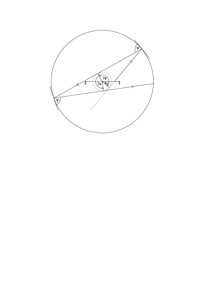
Figure 3: A $\Theta$ billiard with the straight line chosen symmetric with respect to the center of the circle. Initial conditions for a particle orbit in the $\Theta$ billiard are the angular momentum $M$, it i.e., the radius of its caustic (dotted line circle), and the orientation $\theta_{0}$ of its first line segment. The orientation of each line segment of a particle orbit is defined in terms of the total angle covered by the vector pointing from the center of the circle to the point of contact of the line segment with the caustic during its rotation while the particle propagates. In this example the orientation $\theta_{0}$ of the initial line segment is negative and determined by extending the latter back beyond its point of contact with the caustic as indicated in the figure by the dotted line. The angle $\psi$ between the reflected particle orbit and the tangent to the circle boundary at the point of reflection is a constant. At each reflection the orientation angle increases by $2\psi$.

Due to the symmetry of the system it is sufficient to deal with orbits proceeding from the straight line into the right upper quarter of the $\Theta$ billiard. For a given initial orientation $\theta_{0}$ the orbit starts on the horizontal line at a distance $M/\cos\theta_{0}$ from the circle center (see Fig. 3). As we are only interested in orbits starting from the straight line, which reaches from $-r$ to $r$, we obtain as a necessary condition for the initial angle $\theta_{0}$

$$-\chi\leq\theta_{0}\leq\chi$$ (3)

with the notation

$$\chi=\arccos(M/r),$$ (4)

where with Eq. (1),

$$0<\chi\leq\psi.$$ (5)

For an angular momentum $M$ and length $2r$ of the straight line, $\pm\chi$ in Eq. (4) correspond to the initial orientation of those particle orbits which start at the endpoints of the straight line. For a particle starting with an initial orientation $\theta_{0}$ the $n$th line segment of its orbit intersects the horizontal line at $M/\cos\theta_{n}$, if measured with respect to the circle center. Hence, it crosses the straight line, if $-r\leq M/\cos\theta_{n}\leq r$, i.e., if [with Eq. (4)]

$$\theta_{n}\,\mathrm{mod}\,2\pi\in[0;\chi]\cup[\pi-\chi;\pi+\chi]\cup[2\pi-\chi;2\pi]\;,$$ (6)

or equivalently if there is an integer number $m$ such that

$$m\pi-\chi\leq\theta_{n}\leq m\pi+\chi\ ,\ m=0,1,\cdots\ ,$$ (7)

that is, if the distance between $\theta_{n}$ and an integer multiple of $\pi$ is smaller than $\chi$. In order to determine all possible numbers of bounces that particles starting from the straight line perform until they reach it again, we must evaluate this inequality for all allowed initial orientations $\theta_{0}$ [see Eq. (3)] and resulting orientations $\theta_{n}$. With Eq. (3) and Eq. (2) the latter take values from intervals of length $2\chi$ around integer multiples of $2\psi$,

$$n2\psi-\chi\leq\theta_{n}\leq n2\psi+\chi\ ,\ n=0,1,\cdots.$$ (8)

While this inequality defines the range of possible values for the orientations $\theta_{n}$, that in Eq. (7) gives the condition for the intersection of a particle orbit with the straight line after $n$ reflections. Whenever one of the intervals defined in Eq. (8) has common values with one of those given in Eq. (7), a part of all possible orbits reaches the straight line. Thus, the only information we need for the computation of the magic numbers are the orientations of the line segments of a particle orbit. This procedure for the computation of the magic numbers is fast and much more efficient than the reflection program.

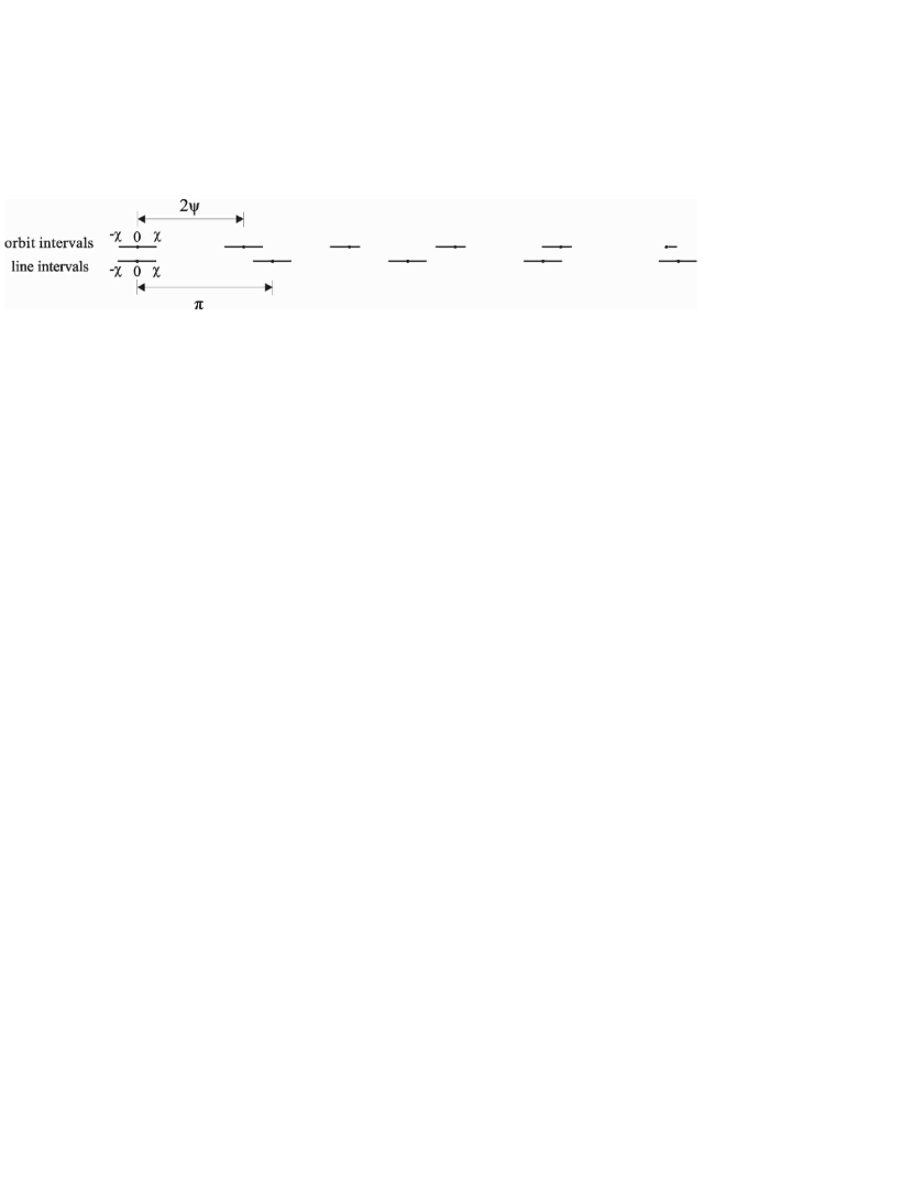
Figure 4: Illustrative representation of particle orbits starting from the straight line in the $\Theta$ billiard in terms of the orientations of their line segments. The orientations of the ensemble of all particle orbits starting from the straight line are restricted to the interval $[-\chi,\chi]$ [see Eq. (3) in the main text]. Their evolution is illustrated by shifting this interval by $2\psi$ at each reflection of the particle with the billiard boundary, thereby obtaining the range of values of the orientations of successive line segments of the particle orbits [see Eq. (8)]. Thus, a string of ”orbit intervals” is obtained. The straight line is represented by a string of ”line intervals” of size $2\chi$ around each multiple of $\pi$ on the angle axis. When an overlap of a line and an orbit interval occurs, the overlapping part of the orbit interval corresponds to angles $\theta_{n}$, which fulfill the inequality Eq. (7), that is, to initial angles $\theta_{0}$, for which the particle orbit ends after $n$ reflections. Accordingly, the overlapping part is cut off the orbit interval in the subsequent iterations.

For a given angular momentum $M$, which defines the angle $\psi$, and length of the straight line $2r$ giving the angle $\chi$, an illustrative graphical representation of this inequality is obtained as follows: All possible initial orientations $\theta_{0}$ of the particle orbits we are interested in take a value from an interval of length $2\chi$ situated symmetrically around 0 [see Eq. (3)]. According to Eq. (8) the orientation $\theta_{n}$ of the $n$th line segment of a particle orbit then takes a value from an interval of length $2\chi$ shifted by $n2\psi$ with respect to the initial interval and by $2\psi$ with respect to that of the preceding line segment, $\theta_{n-1}$. Hence, the orientations of the line segments of all those particle orbits, which start from the straight line, resume values from a string of angle intervals of length $2\chi$ situated at distances of $2\psi$ along the angle axis as depicted in Fig. 4. We call these intervals orbit intervals. Next, let us draw a string of intervals of length $2\chi$ at distances $\pi$ along the angle axis below the string of orbit intervals; we will call these intervals line intervals. While the orbit intervals refer to the inequality Eq. (8) the latter refer to the inequality Eq. (7). The inequality Eq. (7) is fulfilled for a part of the interval of allowed initial angles, whenever one of the orbit and one of the line intervals have common values, i.e., partially overlap. As we are only interested in orbits which start from the straight line, the first orbit interval completely overlaps with the first line interval.

In the example shown in Fig. 4, an orbit interval overlaps with a line interval after the first shift of the orbit interval. Hence, a part of the incoming particles reaches the straight line after one bounce with the circle boundary and the corresponding orbits end there. Accordingly, the orbit interval is shortened by this part. After four reflections, another part of all possible particle orbits reaches the straight line, i.e., the orbit interval is further shortened. The remaining part of the orbit interval overlaps with a line interval after five reflections. Thus, in this example the magic triplet consists of the numbers 1, 4, and 5.

The Eqs. (2) and (6) are related to old results on the so-called circle map slater . On the basis of these results it can be shown that, for a fixed angular momentum, there are at most three magic numbers, and that if there are three magic numbers the largest one is the sum of the two smaller ones. We found an alternative proof of this result which in fact generalizes the translation of orbit and line intervals as depicted in Fig. 4. Using this approach we also obtained the following results: There is a subset of measure zero, where we have only two magic numbers. Further, in the case of the parabolic manifolds described in Ref. altmann only one magic number is finite, whereas the others are infinite and correspond to marginally unstable orbits which never leave the mushroom hat. Finally, in the case of angular momentum zero, all particle orbits intersect the straight line after a single bounce. We thus have exhausted all possibilities. We give in Table 1 the magic triplets for different angular momenta for $r=R/3$ used in Fig. 1(a), and we readily recognize the numbers therein.

Table 1: Magic triplets for different values of angular momentum $M$ for a circular mushroom hat with radius $R$ and half-opening $r=R/3$.

$M$	0.1000	0.5000	0.9000	0.9500	0.9800	0.9950	0.9980	0.9990	0.9992
$n_{1}$	1	1	1	4	5	9	14	14	37
$n_{2}$	4	4	4	5	9	14	23	37	51
$n_{3}$	5	5	5	9	14	23	37	51	88

IV Magic numbers as a function of angular momentum

As the appearance of only one or two magic numbers is restricted to a subset of measure zero in the set of possible angular momenta we must vary the angular momentum in order to investigate them. In Fig. 5 we show the magic numbers as a function of angular momentum for the semicircle mushroom hat with radius $R$ and half-opening $r=R/3$. We observe discontinuities in the behavior of the triplets of time delays (some are marked with arrows in the figure). Precisely there one member of a magic triplet vanishes, such that there are just two magic numbers, and a new magic triplet emerges. The new magic number equals the sum or difference of the other two. This apparently explains the preliminary result that within the whole spectrum of magic numbers each except the two smallest is the sum of two smaller ones.

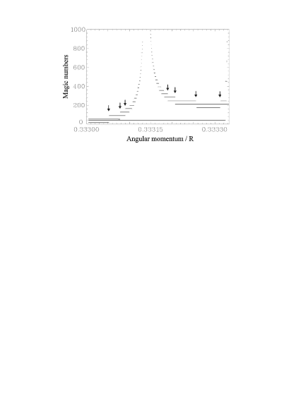
Figure 5: Magic numbers plotted as a function of angular momentum for a semicircle mushroom hat with radius $R$ and a half-opening $r=R/3$ chosen symmetrically with respect to the circle center. The angular momentum is given in units of $R$ as the absolute momentum is set to unity. One observes lines where a magic number remains constant over a certain range of angular momentum values, and sudden discontinuities (arrows), where one member of the triplet changes its value. Note further a singularity, where two of the three members of the triplet tend to infinity. Singularities of this kind are observed at angular momenta of unstable periodic orbits, which do not intersect the straight line in the $\Theta$ billiard in some orientations and do it in others. Between singularities of this kind, every magic number except the first and second, is the sum of two smaller ones, as proven in the text. Note that the chosen interval of angular momentum is small and corresponds to particles which reach the straight line close to one of its ends.

Moreover, we observe a singularity in Fig. 5. It is located at an angular momentum, which is associated with a family of marginally unstable periodic orbits altmann . These periodic orbits are marginally unstable, because the smallest change in angular momentum will cause them to rotate about the circle center and thus eventually to hit the straight line in the $\Theta$ billiard. The smaller the change in angular momentum, the slower this rotation will be, and this must lead to the delay times diverging to infinity as we approach the angular momentum of the periodic orbit. This is clearly seen in Fig. 5. Note that the slopes of the flanks formed by the discontinuities to the left and the right of the angular momentum associated with the singularity are different. Between zero angular momentum and the first singularity as well as in each interval between two singularities only discontinuities of the type discussed above may happen. Therefore, within an interval, each magic number except the two smallest ones at the minimum equals the sum of two smaller magic numbers. However, there is no such relation between magic numbers from two different intervals.

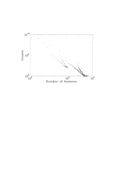
Figure 6: Counts of the numbers of bounce particles starting from the straight line of half-length $r=R/3$ in the $\Theta$ billiard experience with the circle boundary until they reach the straight line again; they were obtained using the linear inequality Eq. (7) for the orientation of line segments between two reflections. Note the persisting selectivity. The organized and regular long time behavior (large number of bounces) is dominated by unstable periodic orbits, while the short time behavior (small number of bounces) cannot be explained by those.

The fact that most magic numbers can be decomposed into two smaller ones, immediately explains why we observe a strong selectivity in the spectra of magic numbers. In Fig. 6 we show the counts of bounce numbers for $r=R/3$ in a double logarithmic plot up to 50000 bounces obtained using Eq. (7). We clearly see that scarcity dominates the picture. Note that the sequence of the magic numbers starts with the Fibonacci like behavior as discussed above. Large magic numbers are dominated by the marginally unstable periodic orbits, which cause two organized sequences of magic numbers with a certain periodicity for each singularity, one for angular momentum values below, the other for values above the singularity. Therefore we understand, why magic numbers may consist of subsets which show a periodicity as observed in Ref. altmann . For our purpose, Fig. 6 teaches us two facts. First, that we are really able to solve the problem also for very large bounce numbers. Second, that the small bounce numbers display a selectivity, that may be accessible to experiments as the allowed numbers typically translate into fairly distinct physical times.

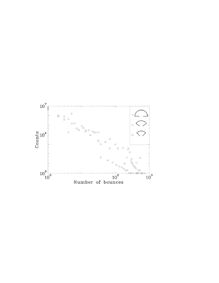
Figure 7: Counts of magic numbers for mushroom hats with half-opening $r=0.3R$ and different shapes: 180^∘-mushroom hat (open triangles), $180^{\circ}\times(\sqrt{5}-1)/2$-mushroom hat (open circles), and 90^∘-mushroom hat (open squares) [see inset and Figs. 1(a) and 1(d)]. Note that the selectivity is observed in all examples, as the density of points remains almost constant in the logarithmic plot. For wider openings there is no correspondence between the number of reflections and the physical time any more.

It turned out that some magic numbers of a mushroom hat can actually be calculated analytically. For every mushroom with a central stem the first magic number equals one, $n_{1}=1$, as in the limiting case of vanishing angular momentum, every orbit leaves the mushroom hat after one reflection. Furthermore, the second magic number of all triplets, whose first magic number is $n_{1}=1$ is given by

$$n_{2}=[\frac{\pi-2\chi}{\pi-2\psi}]\,,$$ (9)

where $[x]$ denotes the integer part of $x$. This result is obtained by evaluating the inequality Eq. (7). It is valid for all triplets with first magic number one, i.e., if

$$M\leq\frac{1}{\sqrt{1+1/r^{2}}}\,.$$

Using the sum rule, the third magic number is given by $n_{3}=n_{2}+1$.

For very small angular momenta, the angles $\psi(M)$ and $\chi(M)$ can be expanded in a Taylor series, leading with Eq. (9) to the simple expressions $n_{1}=1$, $n_{2}=[1/r]+1$, and $n_{3}=[1/r]+2$ for the very first magic triplet within a spectrum of magic numbers of an arbitrary mushroom hat.

V Generalizations to other mushroom billiards

All results presented so far were given for a $180^{\circ}$-mushroom billiard implying a period of $\pi$ for the line intervals. For hats with an angle $\Omega$ smaller than $\pi$ the entire argumentation holds as above except that the period $\pi$ is replaced by $\Omega$. Note that this corresponds to a ”generalized $\Theta$ billiard”, where the straight line rotates each time the straight wall constituting the ”underside” of the hat is hit. If the mushroom hat has an asymmetric opening, the straight line must be shifted even for the $180^{\circ}$-billiard, as the asymmetry is reversed each time the particle hits its underside. The chain of arguments becomes a little more tedious, but still goes through. Thus the description of the dynamics inside the mushroom hat in terms of the translation of orbit and line intervals is indeed general, such that the results hold for a much wider range of mushroom billiards. In Fig. 7 we show bounce numbers in a double logarithmic plot for several angles and openings. The important point is, that we see no qualitative difference in the short time behavior: the selectivity remains in all cases. Furthermore, the magic numbers again combine to triplets (not shown in the figure).

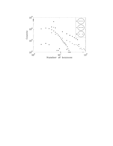
Figure 8: Magic numbers of an elliptic $\Theta$ billiard, corresponding to a mushroom billiard with an elliptic hat [see Fig. 1(b)], with the length of the semimajor axis chosen equal to $R$, that of the semiminor axis equal to $\sqrt{3}/2R$ while the focal points have a distance of $0.5R$ from the center. Circles refer to a straight line chosen symmetrically between the focal points (length $2r=0.99R$), where no selectivity is observed. For a straight line of length $2r=1.1R$ selectivity is evident even for long times, because here only deformed starlike periodic stable orbits of the ellipse survive. Those particles, which intersect the straight line between the focal points, will intersect it again after just one bounce with the elliptic boundary. The diamonds refer to the case of two straight lines of length $0.1R$, whose outer endpoints are located in the focal points. They cut the caustic of the stable orbits of particles crossing the horizontal line between the two focal points from outside. Again a selectivity is observed.

We may finally go one step further and ask, what happens with elliptic hats bunimo4 . There we must remember, that such a hat displays two families of stable particle orbits, one corresponding to particles travelling between the two focal points, the other one to particles surrounding them. We performed numerical calculations for three different choices of the positions of the straight lines for an elliptic $\Theta$ billiard using the reflection program. In the first case, the straight line was positioned between the two focal points and in the second it extends across the focal points. The results are shown in Fig. 8. We see no selectivity in the first case (circles) and a picture very similar to those obtained for the semicircle hats in the second case (crosses). In the second case particles moving on orbits, which start between the focal points all reach the straight line again after only one bounce with the ellipse boundary. The orbits surrounding the two focal points on the other hand are just deformed stars. The line segments of such stars and therefore their elliptic caustic cross the straight line in a way similar to that of those in a circular $\Theta$-billiard. This brought us to the assumption, that a necessary condition for the selectivity is that the opening of the mushroom hat cuts a limiting caustic from outside. In order to confirm this picture we performed a third numerical simulation, where two straight lines were positioned in the elliptic $\Theta$ billiard, which extend from the focal points to the interior (see inset in Fig. 8). In this case the hyperbolic caustic of those stable orbits of particles which cross the horizontal line between the focal points is cut by the straight line from outside, leading indeed again to the selectivity in the magic numbers (diamonds in Fig. 8). Note that these calculations were performed with the simple reflection program. An analysis similar to that for semicircular hats is also possible for elliptic hats, but shall not be carried out here.

VI Conclusion

We have been able to show, that mushroom hats with openings in the straight boundaries have a very selective behavior concerning the number of bounces a particle has with the curved boundary before it escapes. Indeed while the magic number one always occurs we can to some extent design the subsequent numbers and hence the corresponding delay times. We expect that the selectivity of the possible delay times in the hat of the mushroom should show up not only in classical billiards, but also in billiards excited with microwaves. In such experiments the open hat mushroom billiard is excited with a single pulse input signal and the output time signal is expected to be nonperiodic, in contrast to acoustical echoes we know from experience and scattering echoes analyzed in some detail in Refs. mejia ; carlosnjp ; friedrich . This opens new avenues in billiard research. An experimental device for the measurement of delay times in open mushroom billiards can be constructed, based on the analogy between open mushroom hats and the $\Theta$ billiard, with a flat cylindric microwave resonator of circular shape. The straight line defining in the classical billiard the starting and the endpoints of orbits which correspond to particles entering and leaving the mushroom hat can be realized by a strip of microwave absorbing material with an emitting and a receiving antenna positioned close to the strip. To test how the results presented in this paper carry over to wave mechanics, we plan such a microwave experiment with a superconducting cavity proceeding along similar lines as in the one reported in Ref. friedrich in order to investigate the time response. It is though important to repeat, that the equivalence between time and bounce numbers holds only for small openings. Once we have starlike and nonstarlike polygon orbits coexisting the corresponding delay times get mixed, and while the selectivity of bounce numbers may persist, their physical importance may be marginal in this case. Also we must be aware, that the analogy will break down at long times, but these are probably of marginal interest anyway.

Appendix: Magic numbers for fixed angular momentum

In this appendix we shall show that for each value of angular momentum there exist only three magic numbers $n_{l},n_{r}$, and $n_{s}$ where the largest is always the sum of the lower ones, $n_{s}=n_{l}+n_{r}$. For a given length of the straight line and a fixed angular momentum, the angles $\psi$ and $\chi$ can be calculated from Eq. (1) and Eq. (4), where $0<2\psi\leq\pi$ and $0<\chi\leq\psi$ [see Eq. (5)]. The magic numbers are determined by using a procedure based on the inequalities Eq. (7) and Eq. (8) and outlined in the main text.

Now consider Eqs. (2) and (6) which are related to the so-called circle map slater

$$\phi_{n+1}=(\phi_{n}+\alpha)\,\mathrm{mod}\,2\pi\,.$$ (10)

For this map it is known for almost 40 years that angles $\phi_{0}$ originating in a given interval can at most have three different recurrence times, i.e., numbers of iterations for recurrence to the same interval slater . The angle parameter $\alpha$ corresponds to $2\psi$ and $\phi_{n}$ to $\theta_{n}\mathrm{mod}\,2\pi$, i.e., to the orientation of the $n$-th line segment of the particle orbit, where the information on the number of times the particle travelled around the circle center until its $n$-th impact with the circle boundary is dropped (see Eq. (2) and the remark thereafter). Thus this map indicates one for fixed angular momentum and we can use the results presented in slater to argue that, for a fixed angular momentum, we have at most three different delay times.

An intuitive proof of this result is given here based on the translation of the orbit intervals defined in the main text after Eq. (7). This yields an understanding of what happens when the angular momentum varies. As an important further result we shall see that for a fixed angular momentum less than three delay times occur on a subset of measure zero. Since we only consider particle orbits which start on the straight line in the $\Theta$-billiard before their first encounter with the circular boundary, the first orbit interval coincides with the first line interval around zero. The first particles reach the straight line when there is the next partial overlap of an orbit interval with a line interval at the right hand side or at the left hand side. Their particle orbits end there. Accordingly, this part of the orbit interval is cut off the orbit interval in the next shift. The remaining part evolves until the next overlap is reached.

We first proceed to show in (i) that if at the first overlap after $n_{r}$ reflections of the particle at the circle boundary, that is shifts of the orbit interval by $2\psi$, the orbit interval is cut partially from the right hand side and at the second overlap after $n_{l}$ reflections from the left hand side, then the rest of the interval overlaps with a line interval at latest after $n_{s}=n_{r}+n_{l}$ reflections. The same holds in the opposite case when the orbit interval is first cut from the left and then from the right. Next we show in (ii) that it is not possible that the orbit interval is shortened at the same side for the first two subsequent overlaps. As a further step, we demonstrate in (iii) that there is no way to find a further overlap between the first two overlaps and the one after $n_{s}$ reflections. Finally we show, that the possibility of overlapping the complete orbit interval with less than three coincidences of the orbit and a line interval is limitted to a subset of measure zero within the set of all allowed angular momenta.

In order to find the magic numbers it is sufficient to consider the evolution of the orbit interval center ($oc_{n}$) and the line interval center ($lc_{m}$) with increasing numbers of shifts $n=0,1,2,\cdots$ and $m=0,1,2,\cdots$ of the orbit and line intervals, respectively, where $oc_{n}$ is located at $n2\psi$ and $lc_{m}$ at $m\pi$. The $n$-th orbit interval partially overlaps with the $m$-th line interval, if the distance between $oc_{n}$ and $lc_{m}$ is less than the length of the orbit and the line intervals, $2\chi$ [see Eq. (7)]. It is important to note that the length of the orbit and the line intervals is smaller than the distance between two subsequent $oc$’s, $2\chi\leq 2\psi$, and the distance is smaller than that of two subsequent $lc$’s, $2\psi\leq\pi$.

(i) Assume that after $n_{r}$ shifts of the orbit interval and $m_{1}$ shifts of the line interval the distance between $oc_{n_{r}}$ and $lc_{m_{1}}$ is smaller than $2\chi$, and that the orbit interval there partially overlaps at its right end with the line interval. Then $oc_{n_{r}}$ is located to the left of $lc_{m_{1}}$ along the angle axis at a distance $\epsilon_{1}=m_{1}\pi-n_{r}2\psi<2\chi$. The length of the overlapping part of the orbit interval equals $L_{1}=2\chi-\epsilon_{1}$. Further assume, that after $n_{l}$ shifts the remaining part of the orbit interval partially overlaps at its left end with the $m_{2}$-th shift of the line interval. Then $oc_{n_{l}}$ is located to the right of $lc_{m_{2}}$ at a distance $\epsilon_{2}=n_{l}2\psi-m_{2}\pi<2\chi$ and the length of the overlapping part equals $L_{2}=2\chi-\epsilon_{2}$. The length of the remaining part of the orbit interval equals

$$L = 2\chi-L_{1}-L_{2}$$ (11)

$$= \epsilon_{1}+\epsilon_{2}-2\chi$$ (12)

$$= (n_{l}-n_{r})2\psi-(m_{2}-m_{1})\pi-2\chi.$$ (13)

If $L=0$, then already after two overlaps of an orbit with a line interval, all particles will have returned to the straight line, such that there are only two magic numbers; this case will be treated in part (iv) of the proof. The case $L<0$, where more than just the remaining part of the orbit interval overlaps with the line interval, may be excluded, as this would imply that there is another magic number $n^{*}=(n_{l}-n_{r})<n_{l}$ and an $m^{*}=(m_{2}-m_{1})<m_{2}$, where the distance between $oc_{n^{*}}$ and $lc_{m^{*}}$ is less than $2\chi$ [see Eq. (13)], in contradiction to the assumption. For $L>0$, the remaining part is adjacent to the line interval at its left end; its left endpoint is located at a distance $\chi$, its right endpoint at a distance $\epsilon_{1}+\epsilon_{2}-\chi$ from $lc_{m_{2}}$. Exactly as after the first $n_{r}$ and $m_{1}$ shifts of the orbit and the line interval, after $n_{r}$ and $m_{1}$ further shifts of the intervals, the location of $oc_{n_{s}}$ ($n_{s}=n_{r}+n_{l}$), and therefore that of the remaining part, will have moved by a total amount of $\epsilon_{1}$ to the left with respect to $lc_{m_{3}}$ ($m_{3}=m_{1}+m_{2}$) as compared to their initial relative locations, i.e., that of $oc_{n_{l}}$ and $lc_{m_{2}}$. Accordingly, $oc_{n_{s}}$ is located at a distance $|\epsilon_{2}-\epsilon_{1}|$ from $lc_{m_{3}}$, which is smaller than $2\chi$. The left endpoint of the part of the orbit interval that remained after $n_{l}$ shifts, is then located at a distance $|\chi-\epsilon_{1}|$, the right endpoint at a distance $|\epsilon_{2}-\chi|$ from $lc_{m_{3}}$. As both distances are smaller than $\chi$, this part completely overlaps with the line interval. Therefore, provided the orbit interval is first cut at its right, then at its left end at the magic numbers $n_{r}$ and $n_{l}$, the remaining particles all will have reached the straight line again latest after $n_{s}=n_{r}+n_{l}$ shifts of the orbit interval, or equivalently, bounces of the particle with the circle boundary. The same argumentation holds if the interval is first cut from the left and then from the right hand side.

If the first magic number equals 1, as in the example shown in Fig. 4, we already arrived at the end of the proof. In this case, the orbit interval will be cut at its right end after one shift of the line and the orbit interval and $oc_{1}$ will be located at a distance $\epsilon_{1}=\pi-2\psi$ to the left of $lc_{1}$. At each shift $n$ and $m=n$ of the intervals, the distance of $oc_{n}$ from $lc_{m}$, which is located to its right, will increase by an amount $\epsilon_{1}$ until the orbit interval overlaps with the line interval to its left after $n_{l}$ shifts, i.e., until the distance between $oc_{n_{l}}$ and $lc_{n_{l}-1}$ is smaller than $2\chi$. Hence, at the second overlap the orbit interval will be cut at its left end, at a magic number $n_{l}$. Then, as shown in part (i) of the proof, at $n_{s}=n_{l}+1$ all particles will have reached the straight line, and we obtain the magic triplet $1,n_{l},n_{l}+1$. The explicit values can be computed with Eq. (9).

(ii) Assume, that the first magic number is larger than 1 and that the orbit interval overlaps at its left hand side after $n_{l1}$ and again after $n_{l2}$ shifts of oc with respectively the $m_{1}$-th and the $m_{2}$-th line interval. Then, $oc_{n_{l1}}$ and $oc_{n_{l2}}$ will be located to the right of $lc_{m_{1}}$ and $lc_{m_{2}}$, respectively, at a distance

$$\epsilon_{1}=n_{l1}2\psi-m_{1}\pi<2\chi$$ (14)

for the first and

$$\epsilon_{2}=n_{l2}2\psi-m_{2}\pi<2\chi$$ (15)

for the second overlap. The length of the first overlapping part equals $L_{1}=2\chi-\epsilon_{1}$, that of the second $L_{2}=2\chi-\epsilon_{2}$, and the orbit interval will be further shortened at the second overlap only, if $L_{2}$ is larger than $L_{1}$, that is, if $\epsilon_{2}<\epsilon_{1}$. Then

$$0<\epsilon_{1}-\epsilon_{2}=(m_{2}-m_{1})\pi-(n_{l2}-n_{l1})2\psi<2\chi\,.$$ (16)

This implies, that there is another magic number $n^{*}=n_{l2}-n_{l1}<n_{l2}$ and a number $m^{*}=m_{2}-m_{1}$, where the distance $\epsilon_{1}-\epsilon_{2}$ of $oc_{n^{*}}$ from $lc_{m^{*}}$ is less than $2\chi$ (right hand side of the inequality) and the orbit interval is shortened at its right hand side (left hand side of the inequality). This is in contradiction to the assumption.

(iii) Let the orbit interval be shortened at the right hand side after $n_{r}$ reflections and at the left hand side after $n_{l}$ reflections. Assume, that the third magic number is smaller than the sum of the first and second, $n^{*}<n_{r}+n_{l}$. If after $n^{*}$ shifts the orbit interval is shortened again at the left hand side, then, according to (ii), there exists an additional magic number $n^{**}=n^{*}-n_{l}<n_{r}$, where the orbit interval is shortened at the right hand side, in contradiction to the assumption. If on the other hand $n^{*}$ shortens the orbit interval at the right hand side, then, by proceeding as in (ii), it can be shown that there must be another magic number $n^{**}=n^{*}-n_{r}<n_{l}$ where the orbit interval overlaps at the left hand side with a line interval, again in contradiction to the assumption.

(iv) Assume that the orbit interval after $n_{r}$ shifts partially overlaps at its right hand side with a line interval, and after $n_{l}$ shifts the remaining part completely overlaps with a line interval. This situation corresponds to the case $L=0$ in part (i), i.e., if $(n_{l}-n_{r})2\psi-(m_{2}-m_{1})\pi=2\chi$, then there are only two magic numbers. For a given length of the straight line, this equality is fulfilled only for a set of measure zero from the whole set of allowed angular momenta [see Eq. 1) and Eq. (4)]. As we vary the angular momentum for a fixed length of the straight line, the angles $\psi$ and $\chi$ change continuously, and a third magic number emerges because the first and second overlap no longer cover the whole orbit interval. There, we observe a discontinuity in Fig. 5.

The arguments given in this appendix only hold for finite magic numbers. In the case of the parabolic manifolds described in Ref. altmann only one magic number is left finite. The values of angular momentum corresponding to those orbits are also of measure zero in the whole set of possible angular momenta. In Fig. 5, we observe a singularity at these values of angular momentum.

Finally we should note, that the proof also holds, if the line interval is shifted by an arbitrary angle $2\chi<\Omega<\pi$, as we only used the fact, that the length of the orbit and the line interval is smaller than the distance between two subsequent line intervals or orbit intervals.

References

- (1) Ya. G. Sinai, Russ. Math. Surveys 25, 137 (1970).
- (2) C.M. Marcus, A.J. Rimberg, R.M. Westervelt, P.F. Hopkins, and A.C. Gossard, Phys. Rev. Lett. 69, 506 (1992).
- (3) L. Benet and T.H. Seligman, Phys. Lett. A, 273, 331 (2000).
- (4) H.-J. Stöckmann and J. Stein, Phys. Rev. Lett. 64, 2215 (1990).
- (5) E. Doron, U. Smilansky, and A. Frenkel, Phys. Rev. Lett. 65, 3072 (1990).
- (6) S. Sridhar, Phys. Rev. Lett. 67, 785 (1991).
- (7) H.-D. Gräf, H.L. Harney, H. Lengeler, C.H. Lewenkopf, C. Rangacharyulu, A. Richter, P. Schardt, and H.A. Weidenmüller, Phys. Rev. Lett. 69, 1296 (1992).
- (8) S. Deus, P.M. Koch, and L. Sirko, Phys. Rev. E 52, 1146 (1995).
- (9) D.H. Wu, J.S.A. Bridgewater, A. Gokirmak, and S.M. Anlage, Phys. Rev. Lett. 81, 2890 (1998).
- (10) J. Barthelémy, O. Legrand, and F. Mortessagne, Phys. Rev. E 71, 016205 (2005).
- (11) L.A. Bunimovich, Funct. Anal. Appl. 8, 254 (1974).
- (12) B. Eckhardt, J. Phys. A 20, 5971 (1987).
- (13) C. Jung and H. J. Scholz, J. Phys. A 20, 3607 (1987); P. Gaspard and S. Rice, J. Chem. Phys. 90, 2225 (1989); C. Jung and P. Richter, J. Phys. A 23, 2847 (1990).
- (14) L.A. Bunimovich, Chaos 11, 802 (2001).
- (15) C. Jung, T.H. Seligman, and M. Torres, J. non-lin. Math. Phys. Suppl. 12, 404 (2005).
- (16) H.-J. Stöckmann, Quantum Chaos - An Introduction, (Cambridge University Press, Cambridge, 1999).
- (17) A. Richter, in Emerging Applications of Number Theory, The IMA Volumes in Mathematics and its Applications, edited by D.A. Hejhal et al., (Springer, New York, 1999), Vol. 109, p. 479.
- (18) G. Casati, F. Valz–Gris, and I. Guarneri, Lett. Nuovo Cimento Soc. Ital. Fis. 28, 279 (1980).
- (19) M.V. Berry, Ann. Phys. (N.Y.) 131, 163 (1981); “Structures in semiclassical spectra: a question of scale”, in The Wave-Particle Dualism, edited by S. Diner et al, (D. Reidel, Dordrecht, 1984), p. 231.
- (20) O. Bohigas, M.-J. Giannoni, and C. Schmit, Phys. Rev. Lett. 52, 1 (1984).
- (21) F. Leyvraz and T. H. Seligman, Phys. Lett. A 168, 348 (1992).
- (22) M. Sieber and K. Richter, Physica Scripta T90, 128 (2001).
- (23) S. Müller, S. Heusler, P. Braun, F. Haake, and A. Altland, Phys. Rev. Lett. 93, 014103 (2004).
- (24) M. Gutzwiller, J. Math. Phys. 6, 1791 (1970).
- (25) M. Berry and M. Tabor, Proc. R. Soc. London, Ser. A 349, 101 (1976); 356, 375 (1977).
- (26) T.H. Seligman, J.J.M. Verbaarschot, and M. R. Zirnbauer, Phys. Rev. Lett. 54, 215 (1984).
- (27) M. Berry and M. Robnik, Proc. R. Soc. London, Ser. A 400, 229 (1985).
- (28) T.H. Seligman and J.J.M. Verbaarschot, J. Phys. A 18, 2227 (1985).
- (29) R. Blümel, B. Dietz, C. Jung, and U. Smilansky, J. Phys. A 25, 1483 (1992).
- (30) B. Huckestein, R. Ketzmerick, and C.H. Lewenkopf, Phys. Rev. Lett. 84, 5504 (2000).
- (31) C. Jung and T. H. Seligman, J. Phys. A 28, 1507 (1995).
- (32) C. Jung, C. Mejía-Monasterio, O. Merlo, and T. H. Seligman, New J. Phys. 6, 48 (2004).
- (33) C. Jung, C. Mejía-Monasterio, and T.H. Seligman, Europhys. Lett. 55, 616 (2001).
- (34) C. Dembowski, B. Dietz, T. Friedrich, H.-D. Gräf, A. Heine, C. Mejía-Monasterio, M. Miski-Oglu, A. Richter, and T.H. Seligman, Phys. Rev. Lett. 93, 134102 (2004).
- (35) B. Dietz, M. Lombardi, and T.H. Seligman, J. Phys. A 26, L95 (1996).
- (36) L.E. Reichl, The Transition to Chaos (Springer, New York, 2004).
- (37) E.G. Altmann, A.E. Motter, and H. Kantz, Chaos 15, 033105 (2005).
- (38) L. Bunimovich, Chaos 13, 903 (2003); E.G. Altmann, A.E. Motter, and H. Kantz, Phys. Rev. E 73, 026207 (2006); H. Tanaka and A. Shudo, ibid. 74, 036211 (2006).
- (39) N.B. Slater, Proc. Cambridge Philos. Soc. 63, 1115 (1967).
- (40) L. Bunimovich, (Private Communication).
- (41) A. Hobson, J. Math. Phys. 16, 2210 (1975).
- (42) S. Lansel, M. Porter, and L. Bunimovich, Chaos 16, 013129 (2006).