Elastic and inelastic line-soliton solutions of the Kadomtsev-Petviashvili II equation

Abstract

The Kadomtsev-Petviashvili II (KPII) equation admits a large variety of multi-soliton solutions which exhibit both elastic as well as inelastic types of interactions. This work investigates a general class of multi-solitons which were not previously studied, and which do not in general conserve the number of line solitons after interaction. The incoming and outgoing line solitons for these solutions are explicitly characterized by analyzing the $\tau$-function generating such solutions. A special family of $N$-soliton solutions is also considered in this article. These solutions are characterized by elastic soliton interactions, in the sense that amplitude and directions of the individual line solitons as $y\to\infty$ are the same as those of the individual line solitons as $y\to-\infty$. It is shown that the solution space of these elastic $N$-soliton solutions can be classified into $(2N-1)!!$ disjoint sectors which are characterized in terms of the amplitudes and directions of the $N$ line solitons.

1 Introduction

The purpose of this work is to present a characterization of a large family of real, non-singular, line-soliton solutions of the KPII equation

$$(-4u_{t}+u_{xxx}+6uu_{x})_{x}+3u_{yy}=0\,$$ (1.1)

where $u=u(x,y,t)$ and subscripts $x$, $y$ and $t$ denote partial derivatives. The KP equation is perhaps the prototypical (2+1)-dimensional integrable evolution equation originally derived [11] as a model for small-amplitude, long-wavelength, weakly two-dimensional solitary waves in a weakly dispersive medium, and arises in many different applications including water waves and plasmas (for a review, see e.g. [8]). The various aspects related to the integrability of the KP equation have been studied extensively, and a large number of exact solutions have been found. These works are documented in several monographs (see e.g., Refs. [2, 8, 18] and references therein). There are two versions of the KP equation depending on the sign of the dispersion namely, KPI (for positive dispersion) and KPII (for negative dispersion). Here we consider the KPII equation.

Among the exact solutions of KPII, perhaps one of the most well known class of real, non-singular solutions is the line-soliton solutions. The simplest type is the one-soliton solution which is a traveling wave in $xy$-plane, and is localized along a line. A straightforward generalization of this solution to a multi-soliton configuration of $N$ line solitons was also found in earlier works [21, 6]. In the generic case, these $N$-soliton solutions form a pattern of $N$ intersecting straight lines in the $xy$-plane apart from small spatial shifts arising from the pairwise interactions between any two lines. We refer to these solutions as the ordinary $N$-soliton solutions which can be parametrized by $2N$ parameters namely, amplitude and direction (in the $xy$-plane) of the $N$ line solitons. However, it has been shown theoretically and experimentally that it is not possible to obtain ordinary $N$-soliton solutions for all choices of the soliton parameters (see e.g., Ref. [8]). That is, the parameter space of ordinary $N$-soliton solutions is not simply the $N$-fold Cartesian product of the parameter space of one-soliton solution of the KPII equation. Subsequent work has revealed that other families of line soliton solutions exist in addition to the ordinary $N$-soliton solutions. The simplest of these solutions describes the so called “Y-junction” solutions, which describes resonant interaction of two line solitons, and has been known since 1977 [16, 17]. In this case, the three solitons with wave-numbers and frequencies $({\bf k}_{a},\omega_{a}),\,a=1,2,3$, satisfy the three-wave resonance conditions:  ${\bf k}_{1}+{\bf k}_{2}={\bf k}_{3}$ and $\omega_{1}+\omega_{2}=\omega_{3}$. More general resonant solutions have also been obtained in Refs. [15, 19, 20]. Recently, in Ref. [3], the authors found a large family of soliton solutions in which an arbitrary number $N_{-}$ of incoming line solitons interact resonantly via intermediate line solitons which produce web like patterns in the $xy$-plane, and then form an arbitrary number $N_{+}$ of outgoing line solitons, where $N_{-}\neq N_{+}$, in general. We refer to these multi-solitons solutions as the $(N_{-},N_{+})$-soliton solutions of KPII. In particular, the case $N_{-}=N_{+}=N$ yields yet another kind of $N$-soliton solutions which however differ significantly from the ordinary $N$-soliton solutions in their interaction patterns. The current work is motivated by these recent studies which indicate that the solitonic sector of the KPII equation is richer than previously thought as many other families of line-soliton solutions exist in addition to the ordinary $N$-soliton solutions.

In this article we are primarily concerned with the characterization of the incoming and outgoing line solitons of a generic multi-soliton configuration of KPII as well as the classification of a particular class of multi-soliton solutions called the elastic $N$-soliton solutions. The paper is organized as follows. In section 2, we discuss the asymptotic behavior of the $\tau$-function underlying the multi-soliton solutions of KPII. In particular, we show that as $y\to\pm\infty$, the solution $u(x,y,t)$ decays exponentially in the $xy$-plane except along certain rays which correspond to the incoming and outgoing line solitons. We then characterize these asymptotic structures in terms of the parameters of the $\tau$-function. In section 3, we study a special class of solutions called the elastic $N$-soliton solutions. We show that these solutions can be classified into $(2N-1)!!$ inequivalent types determined by the $2N$ soliton parameters comprising of $N$ pairs of amplitudes and directions associated with the incoming or outgoing line solitons. Moreover, from a given set of admissible soliton parameters one can explicitly determine an equivalence class of elastic $N$-soliton solutions such that any two solutions in the equivalence class exhibit similar interaction patterns and have the same set of incoming and outgoing line solitons. In this paper, we only present the results and discuss some of the important features of the multi-soliton solutions of KPII. The proofs of these results and more detailed discussions can be found in Refs. [4, 5].

We point out that the elastic $N$-soliton solutions of KPII equation was also recently addressed in Ref. [12] where an elegant characterization of these solutions were presented in terms of the Schubert cell decomposition of the Grassmann variety Gr($N,2N$). Here we follow a different approach motivated by the physical problem of identifying the distinct types of elastic $N$-soliton solutions with the the corresponding parameter space of soliton amplitudes and velocities. Finally, we note that line soliton solutions with novel web like spatial structures were also found recently in several other $2+1$-dimensional integrable equations. Examples include Refs. [9, 10] for a coupled KP system, and Ref. [13] where similar solutions were found in discrete integrable systems such as the two-dimensional Toda lattice and its fully- and ultra-discrete analogues.

2 Asymptotic line solitons

In this section we investigate the line solitons of the KPII equation and the asymptotic properties of the $\tau$-functions generating such solutions. The solution $u(x,y,t)$ of the KPII equation can be obtained from the $\tau$-function $\tau(x,y,t)$ via the relation

$$u(x,y,t)=2(\log\tau(x,y,t))_{xx}\,.i$$ (2.1)

It is well-known (see, e.g. Refs. [6, 7, 14]) that $\tau(x,y,t)$ can be expressed in the form of a Wronskian

$$\tau(x,y,t)=\mathop{\mathrm{Wr}}\nolimits(f_{1},\dots,f_{N})=\det\begin{pmatrix}f_{1}&f_{2}&\dots&f_{N}\\ f_{1}^{\prime}&f_{2}^{\prime}&\dots&f_{N}^{\prime}\\ \vdots&\vdots&&\vdots\\ f_{1}^{(N-1)}&f_{2}^{(N-1)}&&f_{N}^{(N-1)}\end{pmatrix}\,,$$ (2.2)

where $f_{n}^{(j)}=\partial^{j}f_{n}/\partial x^{j}$, and where the functions $\{f_{n}\}_{n=1}^{N}$ form a set of linearly independent solutions of the linear system

$$f_{y}=f_{xx}\,,\qquad f_{t}=f_{xxx}\,.$$

A general family of multi-soliton solutions can be constructed in a simple way from Eq. (2.2) by choosing each function $f_{n}(x,y,t)$ to be a linear combination of real exponentials. That is,

$$f_{n}(x,y,t)=\mathop{\textstyle\sum}\limits_{m=1}^{M}a_{nm}\,e^{\theta_{m}}\,,\quad n=1,2,\ldots,N\,,$$ (2.3)

where, $\theta_{m}=k_{m}x+k_{m}^{2}y+k_{m}^{3}t+\theta_{0m}\,$ for $m=1,\ldots,M$ are $M$ phases with real phase parameters $k_{1},\ldots,k_{M}$ and real constants $\theta_{01},\dots,\theta_{0M}$, and where the constant coefficients $a_{nm}$ define the $N\times M$ coefficient matrix $A:=(a_{nm})$. Note that one can naturally identify each $f_{n}$ with the $n^{\mathrm{th}}$ row and each phase $\theta_{m}$ with the $m^{\mathrm{th}}$ column of the coefficient matrix $A$, and vice versa. Upon substituting Eq. (2.3) into the Wronskian of Eq. (2.2) and then using the Binet-Cauchy formula to expand the resulting determinant, we obtain the following explicit form of the $\tau$-function

$$\tau(x,y,t)=\mathop{\textstyle\sum}\limits_{1\leq m_{1}<\dots<m_{N}\leq M}A(m_{1},\dots,m_{N})\,\,\exp[\,\theta(m_{1},\dots,m_{N})\,]\!\!\prod_{1\leq s<r\leq N}(k_{m_{r}}-k_{m_{s}})\,,$$ (2.4)

where $A(m_{1},\dots,m_{N})$ is the $N\times N$ minor of $A$ obtained by selecting the columns $1\leq m_{1}<\dots<m_{N}\leq M$, and $\theta(m_{1},\dots,m_{N}):=\theta_{m_{1}}+\ldots+\theta_{m_{N}}$ is a phase combination of $N$ (out of $M$) distinct phases. The $\tau$-function given above could in general, vanish at points $(x,y,t)\in{\mathbb{R}}^{3}$ where the solution $u(x,y,t)$ in Eq. (2.1) would then have singularities. However, the following restrictions on the phase parameters $\{k_{n}\}_{n=1}^{M}$ and on the coefficient matrix $A$ are sufficient to guarantee that the resulting solutions $u(x,y,t)$ of the KPII equation are nonsingular.

Condition 2.1

(Positive definiteness)

1. The phase parameters are distinct. Hence, without loss of generality, they can be ordered as $k_{1}<k_{2}<\ldots<k_{M}$.

2. The $N\times M$ coefficient matrix $A$ satisfies $\mathop{\rm rank}\nolimits(A)=N$, and $M>N$.

3. All non-zero $N\times N$ minors of $A$ are positive.

From Condition 2.1 it is clear that the coefficient of each exponential term of the sum in Eq. (2.4) is positive because the phase parameters $k_{1},\dots,k_{M}$ are well-ordered and all the minors $A(m_{1},\ldots,m_{N})$ of $A$ are also nonnegative. As a result, $\tau(x,y,t)$ is a nonvanishing, positive function for all $(x,y,t)\in{\mathbb{R}}^{3}$, and generates a nonsingular solution of the KPII equation via Eq. (2.1). If $M<N$, $\tau(x,y,t)=0$ because the set of functions $\{f_{n}\}_{n=1}^{M}$ in Eq. (2.2) is linearly dependent; also when $M=N$, $\tau(x,y,t)$ in Eq. (2.4) contains only one exponential term which leads to the trivial solution $u(x,y,t)=0$ in Eq. (2.1). Therefore, for nontrivial solutions we must have $M>N$ when there are more than one exponential term in the sum of Eq. (2.4).

The simplest example is a one-soliton solution obtained by choosing $N=1,\,M=2$ and $f(x,y,t)=e^{\theta_{1}}+e^{\theta_{2}}$, with $k_{1}<k_{2}$. This choice yields the following traveling-wave solution

$$u(x,y,t)={\textstyle\frac{1}{2}}(k_{2}-k_{1})^{2}\mathop{\rm sech}\nolimits^{2}{\textstyle\frac{1}{2}}(\theta_{2}-\theta_{1})=\Phi(\mathbf{k}\cdot\mathbf{x}+\omega t)\,,$$ (2.5)

where $\mathbf{x}=(x,y)$ and where the wave vector $\mathbf{k}:=(l_{x},l_{y})=(k_{1}-k_{2},k_{1}^{2}-k_{2}^{2})$ and the frequency $\omega:=k_{1}^{3}-k_{2}^{3}$ satisfy the nonlinear dispersion relation

$$-4\omega l_{x}+l_{x}^{4}+3l_{y}^{2}=0\,.$$ (2.6)

For fixed $t$, the solution $u(x,y,t)$ decays exponentially in the $xy$-plane except along the line $\theta_{1}=\theta_{2}$ whose normal has a slope $c=l_{y}/l_{x}=k_{1}+k_{2}$. Such solitary wave solutions of the KPII equation are called line solitons. Apart from a trivial constant $\theta_{1,0}-\theta_{2,0}$ in Eq. (2.5) corresponding to an overall translation, a line soliton of KP is characterized by the phase parameters $k_{1},k_{2}$, or by two physical parameters, namely, the soliton amplitude $a:=k_{2}-k_{1}$ and the soliton direction $c:=k_{1}+k_{2}$.

When $c=0$ (i.e., $k_{1}=-k_{2}$), the solution in Eq. (2.5) becomes $y$-independent and reduces to the one-soliton solution of the Korteweg-de Vries (KdV) equation. However, due to the dependence on the additional spatial variable $y$, the multi-soliton solution space of the KPII equation is much richer than that of the KdV. Indeed we find that Eq. (2.3) with the coefficient matrix $A$ satisfying Condition 2.1 leads to a large class of multi-soliton configurations which consist of $N_{-}$ incoming (i.e., as $y\rightarrow-\infty$) and $N_{+}$ outgoing (i.e., as $y\rightarrow\infty$) line solitons. The amplitudes, directions and the number of incoming line solitons are in general different from those of the outgoing line solitons. In order to characterize the incoming and outgoing line solitons associated with these solutions, it is necessary to examine the asymptotic behavior of the $\tau$-function in the $xy$-plane as $|y|\to\infty$, and for finite $t$. Recall from Eq. (2.4) that $\tau(x,y,t)$ is a linear combination of exponential phase combinations with positive coefficients. The leading order behavior of the $\tau$-function as $y\to\pm\infty$ in a given asymptotic sector of the $xy$-plane is governed by that exponential term which is dominant in that region. The solution $u(x,y,t)$ generated by the $\tau$-function is exponentially small at all points in the interior of any dominant region, and is localized only at the boundaries of the dominant regions, where a balance exists between two or more dominant phase combinations in the $\tau$-function of Eq. (2.4). The asymptotic properties of the $tau$-function and the solution $u(x,y,t)$ can be derived from a systematic analysis of these dominant exponential phases. These are summarized below.

Proposition 2.2

For finite values of $t$, and for generic values of phase parameters $k_{1},\ldots,k_{M}$, the incoming and outgoing line solitons of the $(N_{-},N_{+})$-soliton solutions of KPII are characterized as follows.

1. As $y\to\pm\infty$, the dominant phase combinations of the $\tau$-function in adjacent regions of the $xy$-plane contain $N-1$ common phases and differ by only a single phase. The transition between any two such dominant phase combinations $\theta(i,m_{2},\dots,m_{N})$ and $\theta(j,m_{2},\dots,m_{N})$ occurs along the line defined by $L_{ij}:\theta_{i}=\theta_{j}$, where a single phase $\theta_{i}$ in the dominant phase combination is replaced by a phase $\theta_{j}$.

2. Along the single-phase transition line $L_{ij}$, the asymptotic behavior of the $\tau$-function as $y\to\pm\infty$ isdetermined by the balance between the two dominant phase combinations $\theta(i,m_{2},\dots,m_{N})$ and$\theta(j,m_{2},\dots,m_{N})$ in Eq. (2.4), and is given by

   $$\tau(x,y,t)\sim C_{i}\,e^{\theta(i,m_{2},\dots,m_{N})}+C_{j}\,e^{\theta(j,m_{2},\dots,m_{N})}\,.$$

   The coefficients $C_{i}$ and $C_{j}$ above depend on the phase parameters $k_{i},k_{j},k_{m_{2}},\ldots,k_{m_{N}}$, and on the $N\times N$ minors $A(i,m_{2},\dots,m_{N})$ and $A(j,m_{2},\dots,m_{N})$ of the coefficient matrix $A$. The asymptotic behavior of the solution in a neighborhood of a single-phase transition is then obtained from Eq. (2.1) as

   $$u(x,y,t)\sim{\textstyle\frac{1}{2}}(k_{i}-k_{j})^{2}\mathop{\rm sech}\nolimits^{2}\big{[}{\textstyle\frac{1}{2}}(\theta_{i}-\theta_{j})\big{]}\,,$$ (2.7)

   which is a traveling wave satisfying the dispersion relation in Eq. (2.6). Equation (2.7) has the same form as the one-soliton solution in Eq. (2.5), and thus it defines an asymptotic (incoming or outgoing) line soliton associated with the single-phase transition $i\to j$. For each asymptotic line soliton, the soliton amplitude is given by $a_{ij}=|k_{i}-k_{j}|$, and the soliton direction is given by $c_{ij}=k_{i}+k_{j}$, which the direction (slope of the normal vector) of the transition line $L_{ij}$.

We can label each asymptotic line soliton associated with the single-phase transition $i\to j$, by the index pair $[i,j]$ which uniquely identifies the phase parameters $k_{i}$ and $k_{j}$ in the ordered set $\{k_{1},\dots,k_{M}\}$.

 

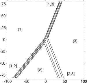
Figure 2.1: Dominant phase combinations in the different regions of the $x,y$-plane (labeled by the indices in parentheses) and the asymptotic line solitons (labeled by the indices in square braces) for two different line soliton solutions: (a) a Miles resonant solution (Y-junction) with $(k_{1},k_{2},k_{3})=(-\frac{3}{2},-\frac{1}{2},\frac{1}{2},2)$ at $t=0$; (b) an inelastic $(2,2)$-soliton with $(k_{1},\dots,k_{4})=(-\frac{3}{2},-\frac{1}{2},0,1)$ at $t=0$. Here and in all of the following figures, the horizontal and vertical axes are respectively $x$ and $y$, and the graphs show contour lines of $\log u(x,y,t)$ at a fixed value of $t$.

The simplest instance of a transition of dominant phase combinations arises for the one-soliton solution (2.5), which is localized in the $xy$-plane along the line $\theta_{1}=\theta_{2}$ defining the boundary of the two half-planes where each of the two phases $\theta_{1}$ and $\theta_{2}$ dominates. In the general case, the dominant regions are more complicated although the solution $u(x,y,t)$ is still localized along the boundaries of these regions. For example, Fig. 2.1(a) illustrates a $(2,1)$-soliton solution mentioned in the introduction as a Y-junction [16] describing the resonant interaction of two line solitons. This solution corresponds to $N=1,\,M=3$, and is generated by the $\tau$-function $\tau(x,y,t)=e^{\theta_{1}}+e^{\theta_{2}}+e^{\theta_{3}}$. In this case, the $xy$-plane is partitioned into three dominant regions corresponding to each of the dominant phases $\theta_{1}$, $\theta_{2}$ and $\theta_{3}$. Once again, the solution $u(x,y,t)$ is exponentially small in the interior of each dominant regions, and is localized along the phase transition boundaries: $\theta_{1}=\theta_{2}$, $\theta_{1}=\theta_{3}$ and $\theta_{2}=\theta_{3}$. Each of the asymptotic line solitons labeled by the index pairs [1,2], [2,3] and [1,3] are given by Eq. (2.7) and satisfy the one-soliton dispersion relation Eq. (2.6). While some of the dominant regions have infinite extensions in the $xy$-plane, others can be bounded, as in the case of the $(2,2)$-soliton shown in Fig. 2.1(b). This solution is generated by the $\tau$-function in Eq. (2.2) with $f_{1}=e^{\theta_{1}}-e^{\theta_{4}}$ and $f_{2}=e^{\theta_{2}}+e^{\theta_{3}}+e^{\theta_{4}}$, i.e., $N=2,\,M=4$. In addition to the unbounded dominant regions corresponding to the phase combinations $\theta(1,2),\,\theta(1,4),\,\theta(3,4)$ and $\theta(1,3)$, in this case there is also a bounded region in the $xy$-plane where $\theta(2,4)$ is the dominant phase combination. The boundaries of this region is formed by the incoming asymptotic line solitons [1,4] and [2,3], together with the intermediate line soliton [1,2]. Note that the outgoing line solitons [1,3] and [2,4] interact resonantly via two Y-junctions, while the incoming soliton pair interact non-resonantly. Note also that the intermediate segment is a line soliton in its own right, since the solution is locally given by Eq. (2.7), with $[i,j]=[2,3]$.

According to Proposition 2.2, an asymptotic line soliton corresponds to a dominant balance between two phase combinations in the $\tau$-function. But one still needs to identify which particular phase combinations are indeed dominant in a given $\tau$-function as $|y|\to\infty$. This requires a closer examination at the structure of the $N\times M$ coefficient matrix $A$ associated with the $\tau$-function. Note that elementary row operations on $A$ given by $A\rightarrow A^{\prime}=G\,A$ where $G\in\mathrm{GL}(N,{\mathbb{R}})$, amounts to an overall rescaling of the $\tau$-function in Eq. (2.4), i.e., $\tau(x,y,t)\to\tau^{\prime}(x,y,t)=\det(G)\,\tau(x,y,t)$. Since such rescaling leaves the solution $u(x,y,t)$ in Eq. (2.1) invariant, it is possible to choose the coefficient matrix $A$ in reduced row-echelon form (RREF) making use of Gaussian elimination. Recall that, for an $N\times M$ matrix in RREF, the leftmost nonvanishing entry in each nonzero row is called a pivot, which is normalized to 1, so that the pivot columns are the elements of the canonical basis of ${\mathbb{R}}^{N}$. Throughout the rest of this work we will consider the coefficient matrix $A$ to be in RREF, and to satisfy Condition 2.1 and the following additional conditions:

Condition 2.3

(Irreducibility)  Each column of $A$ contains at least one nonzero element, and each row of $A$ contains at least one nonzero element in addition to the pivot.

Then a detailed analysis of the coefficient matrix $A$ satisfying Conditions 2.1 and 2.3 leads to an explicit identification of those $i\to j$ single-phase transitions which actually occurs as $|y|\to\infty$, for any given $\tau$-function of Eq. (2.4). As a result, each asymptotic line-soliton $[i,j]$ is also explicitly determined by the coefficient matrix $A$. as given below. Specifically, we have the following results.

Proposition 2.4

Each index pair $[i,j]$ labeling an asymptotic line soliton of a $(N_{-},N_{+})$-soliton solution are uniquely identified with a pair of columns of the associated coefficient matrix $A$, as prescribed below.

1. An asymptotic line soliton as $y\to\infty$ is identified by a unique index pair $[e_{n},j_{n}]$ with $e_{n}<j_{n}$ and where $\{e_{n}\}_{n=1}^{N}$ label the pivot columns of $A$. Similarly, an asymptotic line soliton as $y\to-\infty$ is identified with a unique index pair $[i_{n},g_{n}]$ with $i_{n}<g_{n}$ and where $\{g_{n}\}_{n=1}^{M-N}$ label the non-pivot columns of $A$. Thus, the $(N_{-},N_{+})$-line soliton solution of KPII generated from the $\tau$-function in Eq. (2.4) has exactly $N_{+}=N$ asymptotic line solitons as $y\to\infty$ and $N_{-}=M-N$ asymptotic line solitons as $y\to-\infty$.

2. The necessary and sufficient conditions for an index pair $[i,j]$ to identify an asymptotic line soliton is determined by considering the ranks of two sub-matrices $X_{ij}$ and $Y_{ij}$ of $A$. They can be denoted by their column indices as follows:

   $$X_{ij}=\left[1,2,\ldots,i-1,j+1,\ldots,M\right]\qquad Y_{ij}=\left[i+1,\ldots j-1\right]\,.$$

   That is, $X_{ij}$ consists of all consecutive columns to the left of the i^th column and all consecutive columns to the right of the j^th column of $A$, while $Y_{ij}$ consists of all consecutive columns in between the i^th and j^th column of $A$. The rank conditions are then stated as follows.

   1. $[i,j]$ identifies an asymptotic line soliton as $y\to\infty$ if and only if  $\mathop{\rm rank}\nolimits(X_{ij}):=r\leq N-1$  and $\mathop{\rm rank}\nolimits(X_{ij}|i)=\mathop{\rm rank}\nolimits(X_{ij}|j)=\mathop{\rm rank}\nolimits(X_{ij}|i,j)=r+1$.

   2. $[i,j]$ identifies an asymptotic line soliton as $y\to-\infty$ if and only if   $\mathop{\rm rank}\nolimits(Y_{ij}):=s\leq N-1$  and $\mathop{\rm rank}\nolimits(Y_{ij}|i)=\mathop{\rm rank}\nolimits(Y_{ij}|j)=\mathop{\rm rank}\nolimits(Y_{ij}|i,j)=s+1$.

   Above, $(Z|m,n)$ denotes the sub-matrix $Z$ of $A$ augmented by the columns $m$ and $n$ of $A$.

Note that for the asymptotic line soliton $[e_{n},j_{n}]$ as $y\to\infty$ in Proposition 2.4(i), $e_{n}$ is a pivot index but the index $j_{n}$ can be either a pivot or a non-pivot index. Similarly, for the asymptotic line solitons $[i_{n},g_{n}]$ as $y\to-\infty$, the index $g_{n}$ is an non-pivot index, while $i_{n}$ can be either a pivot or a non-pivot index. The necessary and sufficient rank conditions in Proposition 2.4(ii) provides a constructive method to identify the asymptotic line solitons as $y\to\pm\infty$ from a given coefficient matrix $A$ in RREF. We illustrate these statements by the examples below.

Example 1:  Consider the $\tau$-function in Eq. (2.4) with $N=2$ and $M=5$ generated by the coefficient matrix

$$A=\begin{pmatrix}1&1&0&\!-1&\!-2\\ 0&0&1&1&1\end{pmatrix}$$ (2.8)

The pivot columns of $A$ are labeled by the indices $\{e_{1},e_{2}\}=\{1,3\}$, and the non-pivot columns by the indices $\{g_{1},g_{2},g_{3}\}=\{2,4,5\}$. Thus, from Proposition 2.4(i) we know that there will be $N_{+}=N=2$ asymptotic line solitons as $y\to\infty$, identified by the index pairs $[1,j_{1}]$ and $[3,j_{2}]$ for some $j_{1}>1$ and $j_{2}>3$, and that there will be $N_{-}=M-N=3$ asymptotic line solitons as $y\to-\infty$, identified by the index pairs $[i_{1},2]$, $[i_{2},4]$ and $[i_{3},5]$, for some $i_{1}<2$, $i_{2}<4$ and $i_{3}<5$. We first determine the asymptotic line solitons as $y\to\infty$ using the rank conditions prescribed in Proposition 2.4(ii). For the first pivot column, $e_{1}=1$, we start with $j=2$ and consider the sub-matrix $X_{12}=\bigl{(}\begin{smallmatrix}0&\!-1&\!-2\\ 1&1&1\end{smallmatrix}\bigr{)}\,$. Since $\mathop{\rm rank}\nolimits(X_{12})=2$ which is greater than $N-1=1$, we conclude that the pair $[1,2]$ cannot identify an asymptotic line soliton as $y\to\infty$. Incrementing $j$ to $j=3,4,5$ and checking the rank of each sub-matrix $X_{1j}$ we find that the rank conditions in Proposition 2.4(ii) are satisfied when $j=4$: $X_{14}=\bigl{(}\begin{smallmatrix}\!-2\\ 1\end{smallmatrix}\bigr{)}$, so $\mathop{\rm rank}\nolimits(X_{14})=1$ and $\mathop{\rm rank}\nolimits(X_{14}|1)=\mathop{\rm rank}\nolimits(X_{14}|4)=\mathop{\rm rank}\nolimits(X_{14}|1,4)=2$. Thus, the first asymptotic line soliton as $y\to\infty$ is identified by the index pair $[1,4]$. For the second pivot, $e_{2}=3$, proceeding in a similar manner we find that $j=4$ does not satisfy the rank conditions (since $X_{34}$ has rank 2) but $j=5$ does: $X_{35}=\bigl{(}\begin{smallmatrix}0&\!-1&\!-2\\ 1&1&1\end{smallmatrix}\bigr{)}\,$, which yields $\mathop{\rm rank}\nolimits(X_{35})=1$ and $\mathop{\rm rank}\nolimits(X_{35}|3)=\mathop{\rm rank}\nolimits(X_{35}|5)=\mathop{\rm rank}\nolimits(X_{35}|3,5)=2$. Therefore, the asymptotic line solitons as $y\to\infty$ are given by the index pairs $[1,4]$ and $[3,5]$.

 

Figure 2.2: Line soliton solutions of KPII: (a) the (3,2)-soliton solution generated by the coefficient matrix $A$ in Eq. (2.8) with $(k_{1},\dots,k_{5})=(-1,0,\frac{1}{4},\frac{3}{4},\frac{5}{4})$ at $t=-32$; (b) the (3,3)-soliton solution generated by the coefficient matrix $A$ in Eq. (2) with $(k_{1},\dots,k_{6})=(-1,-\frac{1}{2},0,\frac{1}{2},1,\frac{3}{2})$ at $t=20$.

Next we consider the asymptotics for $y\to-\infty$. Starting with the non-pivot column $g_{1}=2$, the only column to its left is $i=1$. Then, we have $Y_{12}=\emptyset$, and $\mathop{\rm rank}\nolimits(Y_{12}|1)=\mathop{\rm rank}\nolimits(Y_{12}|2)=\mathop{\rm rank}\nolimits(Y_{12}|1,2)=1$. Consequently, the pair $[1,2]$ identifies an asymptotic line soliton as $y\to-\infty$. For $g_{2}=4$ we consider $i=1,2,3$ and find that the rank conditions are satisfied only for $i=2$. In this case, $Y_{24}=\bigl{(}\begin{smallmatrix}0\\ 1\end{smallmatrix}\bigr{)}$, so $\mathop{\rm rank}\nolimits(Y_{24})=1=N-1$ and $\mathop{\rm rank}\nolimits(Y_{24}|2)=\mathop{\rm rank}\nolimits(Y_{24}|4)=\mathop{\rm rank}\nolimits(Y_{24}|2,4)=2$. Hence $[2,4]$ is the unique asymptotic line soliton as $y\to-\infty$ associated to the non-pivot column $g_{2}=4$. In a similar way, we can uniquely identify the last asymptotic line soliton as $y\to-\infty$ as given by the indices $[3,5]$. To summarize, there are $N_{+}=2$ outgoing line solitons given by the index pairs $[1,4]$ and $[3,5]$, and there are $N_{-}=3$ incoming line solitons given by the index pairs $[1,2]$, $[2,4]$ and $[3,5]$. A snapshot of the solution at $t=-32$ is shown in Fig. 2.2.

Example 2:  Next, consider the $\tau$-function with $N=3$ and $M=6$ generated by the coefficient matrix in RREF

$$A=\begin{pmatrix}1&1&1&0&0&0\\ 0&0&0&1&0&\!-1\\ 0&0&0&0&1&2\end{pmatrix}\,.$$

Again, we first determine the asymptotic line solitons as $y\to\infty$. In this case, the pivot columns of $A$ are labeled by $\{e_{1},e_{2},e_{3}\}=\{1,4,5\}$. So, the asymptotic line solitons as $y\to\infty$ are given by the index pairs $[1,j_{1}]$, $[4,j_{2}]$ and $[5,j_{3}]$ for some $j_{1},\,j_{2},\,j_{3}$. Starting with the first pivot, $e_{1}=1$, we take $j=2,3,\dots$ and check the rank of the sub-matrix $X_{ij}$ in each case. When $j=2$ we have $X_{12}=\left(\!\begin{smallmatrix}1&0&0&0\\ 0&1&0&\!-1\\ 0&0&1&2\end{smallmatrix}\!\right)\,$, so $\mathop{\rm rank}\nolimits(X_{12})=3>N-1$. Hence, according to Proposition2.4(ii), the index pair $[1,2]$ does not correspond to an asymptotic line soliton as $y\to\infty$. We then take $j=3$ and consider the sub-matrix $X_{13}=\left(\!\begin{smallmatrix}1&0&0\\ 0&0&\!-1\\ 0&1&2\end{smallmatrix}\!\right)\,$. Since $\mathop{\rm rank}\nolimits(X_{13})=2$ and $\mathop{\rm rank}\nolimits(X_{13}|1)=\mathop{\rm rank}\nolimits(X_{13}|3)=\mathop{\rm rank}\nolimits(X_{13}|1,3)=3$, the rank conditions in Proposition2.4(ii) are satisfied. Therefore the index pair $[1,3]$ corresponds to an asymptotic line soliton as $y\to\infty$. Moreover, by considering $j=4,5,6$ one can easily check that the rank conditions are no longer satisfied. Thus $[1,3]$ is the unique asymptotic line soliton associated with the pivot index $e_{1}=1$ as $y\to\infty$. Proceeding in a similar way, we find that for the pivot column $e_{2}=4$, the rank conditions are only satisfied when $j=5$, since $X_{45}=\left(\!\begin{smallmatrix}1&1&1&0\\ 0&0&0&\!-1\\ 0&0&0&2\end{smallmatrix}\!\right)\,$, is of rank 2, and $\mathop{\rm rank}\nolimits(X_{45}|4)=\mathop{\rm rank}\nolimits(X_{45}|5)=\mathop{\rm rank}\nolimits(X_{45}|4,5)=3$. Therefore, the index pair $[4,5]$ corresponds to an asymptotic line soliton as $y\to\infty$. Finally, we find that the third asymptotic line soliton as $y\to\infty$ is given by the index pair $[5,6]$.

Next, we proceed to determine the asymptotic line solitons as $y\to-\infty$. The non-pivot columns of $A$ are labeled by the indices $g_{1}=2$ $g_{2}=3$ and $g_{3}=6$. For $g_{1}=2$, the only possible value of $i<j$ is $i=1$. In this case $Y_{12}=\emptyset$, so $\mathop{\rm rank}\nolimits(Y_{12})=0$ and $\mathop{\rm rank}\nolimits(Y_{12}|1)=\mathop{\rm rank}\nolimits(Y_{12}|2)=\mathop{\rm rank}\nolimits(Y_{12}|1,2)=1$. Thus, the pair $[1,2]$ identifies an asymptotic line soliton as $y\to-\infty$. For $g_{2}=3$ we consider $i=2,1$. When $i=2$, the rank conditions in Proposition 2.4(ii) are satisfied, leading to the asymptotic line soliton $[2,3]$ as $y\to-\infty$. Similarly, it is easy to verify that for $g_{3}=6$ the index pair $[4,6]$ uniquely identifies the asymptotic line soliton as $y\to-\infty$. Summarizing, there are $N_{+}=3$ asymptotic line solitons as $y\to\infty$ identified by the index pairs $[1,3]$, $[4,5]$ and $[5,6]$, and there are $N_{-}=3$ asymptotic line solitons as $y\to-\infty$ identified by the index pairs $[1,2]$, $[2,3]$ and $[4,6]$. A snapshot of this $(3,3)$-soliton solution at $t=-20$ is shown in Fig. 2.2b.

So far we have discussed the properties of the generic $(N_{-},N_{+})$-soliton solutions of KPII, and have shown how to characterize the asymptotic line solitons as $y\to\pm\infty$ from the corresponding $\tau$-function. In the next section, we investigate an important subclass of the $(N_{-},N_{+})$-soliton solutions called the elastic $N$-soliton solutions.

3 Elastic $N$-soliton solutions

We begin this section by introducing the notion of equivalence classes of soliton solutions and their $\tau$-functions, both of which will play important roles in this section.

Definition 3.1

(Equivalence class)  Let $\Theta$ denote the set of all exponential phase combinations whose coefficients are non-zero in the $\tau$-function of Eq. (2.4). Two $tau$-functions are said to be in the same equivalence class if they contain the same set $\Theta$ (up to an overall exponential phase factor). All $(N_{-},N_{+})$-soliton solutions of KPII generated by an equivalence class of $\tau$-functions form an equivalence class of solutions.

It is clear from the above definition that the $\tau$-functions in a given equivalence class can be viewed as positive-definite sums of the same exponential phase combinations but with different sets of coefficients. Such $\tau$-functions are parametrized by the same set of phase parameters $k_{1},\ldots,k_{M}$, but the constants $\theta_{m0}$ in the phase $\theta_{m}$ are different. Moreover, the irreducible coefficient matrices associated with the $\tau$-functions have exactly the same sets of vanishing and non-vanishing minors, but the magnitudes of the non-vanishing minors are different for different matrices. Then, an important consequence of Proposition 2.2 is that for all $(N_{-},N_{+})$-soliton solutions in the same equivalence class, the corresponding asymptotic line solitons arise from the same $i\to j$ single-phase transition, and are therefore labeled by the same index pair $[i,j]$. Proposition 2.4 then implies that the coefficient matrices associated with the $\tau$-functions in the same equivalence class have identical sets of pivot and non-pivot indices which identify respectively, the asymptotic line solitons as $y\to\infty$ and as $y\to-\infty$. Thus, solutions in the same equivalence class can differ only in the position of each asymptotic line solitons and in the location of each interaction vertex. As a result, any $(N_{-},N_{+})$-soliton solution of KPII can be transformed into any other solution in the same equivalence class by spatio-temporal translations of the individual asymptotic line solitons.

The KPII equation (1.1) is invariant under the symmetry $(x,y,t)\to(-x,-y,-t)$. Thus, if $u(x,y,t)$ is an $(M-N,N)$-soliton solution of KPII, then $u(-x,-y,-t)$ is also an $(N_{-},N_{+})$-soliton solution whose incoming and outgoing line solitons are reversed so that $N_{-}=N$ and $N_{+}=M-N$. In general, $u(x,y,t)$ and $u(-x,-y,-t)$ belong to two different equivalence classes of solutions, and so do their generating $\tau$-functions. However, the function $\tau(-x,-y,-t)$ generating the solution $u(-x,-y,-t)$ is not by itself a $\tau$-function according to Eq. (2.4). Using Eq. (2.4), $\tau(-x,-y,-t)$ can be expressed as $\tau(-x,-y,-t)=e^{-\theta_{1,\dots,M}}\,\tau^{\prime}(x,y,t)\,,$ where the function

$$\tau^{\prime}(x,y,t)=\!\!\!\mathop{\textstyle\sum}\limits\limits_{1\leq m_{1}<\dots<m_{N}\leq M}\!\!\!A(m_{1},\dots,m_{N})\,\,\exp[\theta(l_{1},\dots,l_{M-N})]\!\!\!\prod_{1\leq s<r\leq N}(k_{m_{r}}-k_{m_{s}})$$

is a positive definite sum of exponential phase combinations labeled by the set of indices $\{l_{1},\ldots,l_{M-N}\}$, which is the complement of $\{m_{1},\ldots,m_{N}\}$ in $\{1,2,\ldots,M\}$. Moreover, since $\tau^{\prime}(x,y,t)$ only differs from $\tau(-x,-y,-t)$ by an overall exponential phase factor, it should be clear from Eq. (2.1) that they both generate the same solution $u(-x,-y,-t)$. The correspondence between equivalence classes of solutions and their $\tau$-functions related via the symmetry $(x,y,t)\to(-x,-y,-t)$ leads to the following notion of duality.

Definition 3.2

(Duality)  Two equivalence classes of $\tau$-functions are said to be dual if they are parametrized by the same set of phase parameters $\{k_{1},k_{2},\ldots,k_{M}\}$, but correspond to complementary sets of exponential phase combinations $\Theta$ and $\Theta^{\prime}$. That is,

$$\theta(m_{1},\ldots,m_{N})\in\Theta\,\,\Leftrightarrow\,\,\theta(l_{1},\ldots,l_{M-N})\in\Theta^{\prime}\,,$$

where the sets $\{m_{1},\ldots,m_{N}\}$ and $\{l_{1},\ldots,l_{M-N}\}$ form a disjoint partition of the integers $\{1,2,\ldots,M\}$. Similarly, two equivalence classes of $(N_{-},N_{+})$-soliton solutions are dual if they are generated by dual equivalence classes of $\tau$-functions.

In particular, if a given $(M-N,N)$-soliton solution $u(x,y,t)$ belongs to a certain equivalence class, then the corresponding $(N,M-N)$-soliton solution $u(-x,-y,-t)$ belongs to the dual equivalence class.

An interesting subclass of $(N_{-},N_{+})$-soliton solutions are the elastic $N$-soliton solutions of KPII as mentioned in section 1. These can be defined as follows.

Definition 3.3

A $(N_{-},N_{+})$-soliton solution is called elastic if it belongs to an equivalence class which is its own dual.

Clearly, in this case we have $N_{+}=N_{-}=N$ and $M=2N$. Moreover, the amplitudes and directions of the $N$ incoming line solitons coincide with those of the $N$ outgoing line solitons. Thus, an elastic $N$-soliton solution is generated by a “self-dual” $\tau$-function which is a positive definite sum over a set $\Theta$ of exponential phase combinations such that the following condition holds:

$$\theta(m_{1},\ldots,m_{N})\in\Theta\,\,\Leftrightarrow\,\,\theta(l_{1},\ldots,l_{N})\in\Theta\,,\quad\forall\,\{m_{1},\ldots,m_{N}\}\sqcup\{l_{1},\ldots,l_{N}\}=\{1,2,\ldots,2N\}\,.$$

We outline below the main properties of the elastic $N$-soliton solutions. Additional details regarding these solutions can be found in Refs. [5, 12].

Proposition 3.4

The elastic $N$-soliton solutions of KPII are characterized as follows.

1. Each elastic $N$-soliton solution $u(x,y,t)$ and the dual solution $u(-x,-y,-t)$ belong to the same equivalence class.

2. The $\tau$-function corresponding an elastic $N$-soliton solution has $M=2N$ distinct phase parameters and an $N\times 2N$, irreducible, rank $N$ coefficient matrix $A$ whose $N\times N$ minors satisfy the duality conditions:

   $$A(m_{1},\ldots,m_{N})=0\,\,\Leftrightarrow\,\,A(l_{1},\ldots,l_{N})=0\,,$$ (3.1)

   where the indices $\{m_{1},\ldots,m_{N}\}$ and $\{l_{1},\ldots,l_{N}\}$ form a disjoint partition of integers $\{1,2,\ldots,2N\}$.

3. Each elastic $N$-soliton solution exactly $N$ asymptotic line solitons as $y\to\pm\infty$ identified by the same index pairs $[e_{n},g_{n}]$ with $e_{n}<g_{n},\,n=1,\ldots,N$. The indices $e_{1},e_{2},\ldots,e_{N}$ and $g_{1},g_{2},\ldots,g_{N}$ label respectively, the pivot and non-pivot columns of the coefficient matrix $A$. Hence, they form a disjoint partition of integers $\{1,2,\ldots,2N\}$.

4. The amplitude and direction of the $n^{\mathrm{th}}$ asymptotic line soliton $[e_{n},g_{n}]$ are the same as $y\to\pm\infty$, and are given in terms of the phase parameters as $a_{n}=k_{g_{n}}-k_{e_{n}}$ and $c_{n}=k_{g_{n}}+k_{e_{n}}$.

The set $S_{N}:=\{(a_{n},c_{n})|a_{n}>0\}_{n=1}^{N}\subset{\mathbb{R}}^{2N}$ of all admissible $N$-tuples of amplitude-direction pair associated with elastic $N$-soliton solution will be called the soliton parameter space. An element $\{a_{n},c_{n}\}_{n=1}^{N}\in S_{N}$ of soliton parameters is admissible, if it yields a set of $2N$ distinct phase parameters $K_{N}:=\{k_{n}^{\pm}\}_{n=1}^{N}$ where $k_{n}^{\pm}=(c_{n}\pm a_{n})/2$ and $k_{n}^{-}<k_{n}^{+}$. By sorting the elements of $K_{N}$ in increasing order $k_{1}<\ldots<k_{2N}$, one obtains the ordered set $K=\{k_{1},k_{2},\ldots,k_{2N}\}$ of phase parameters associated with the $\tau$-function. The positions of the phase parameters $k_{n}^{\pm}$ of the $n^{\mathrm{th}}$ line soliton can be labeled uniquely within the ordered set $K$ by an ordered pair of indices $[i_{n},j_{n}]$ such that $i_{n}<j_{n}$. That is, $k_{n}^{-}=k_{i_{n}},\,k_{n}^{+}=k_{j_{n}}$. Since $[i_{n},j_{n}]$ also identify two distinct columns of the coefficient matrix $A$, it follows that $i_{n}=g_{n}$ which labels a pivot column, and $j_{n}=g_{n}$ which labels a non-pivot column of $A$, for elastic $N$-soliton solutions. We refer to this identification between the sets $K_{N}$ and $K$ as phase pairing which defines a map $S_{N}\rightarrow S$, where $S$ is the set of all possible choices of $N$ distinct integer pairs $\{[i_{n},j_{n}]\}_{n=1}^{N}$ from $\{1,2,\ldots,2N\}$. This map identifies each set of soliton parameters $\{(a_{n},c_{n})\}_{n=1}^{N}\in S_{N}$ to a set $\{[e_{n},g_{n}]\}_{n=1}^{N}\in S$ of (pivot, non-pivot) index pairs. Note however that distinct elements of $S_{N}$ can in fact lead to the same pairing if the elements of the corresponding sets $K_{N}$ are ordered in exactly identical fashion. Thus, phase pairing induces a partition of the soliton parameter space $S_{N}$ into several disjoint sectors. Each sector is distinguished by a single element $\{[e_{n},g_{n}]\}_{n=1}^{N}\in S$ of distinct integer pairs which labels the $N$ asymptotic line solitons corresponding to any set $\{(a_{n},c_{n})\}_{n=1}^{N}$ of soliton parameters chosen from that sector in $S_{N}$. Therefore, the total number of such disjoint sectors is given by the number of elements of the set $S$ namely, $|S|=(2N-1)!!$. Furthermore, given any set of soliton parameters $\{(a_{n},c_{n})\}_{n=1}^{N}$ from one of these sectors in $S_{N}$, it is possible to construct a coefficient matrix $A$ in RREF satisfying Conditions 2.1 and 2.3 and whose pivot and non-pivot columns are labeled by the corresponding set of index pairs $\{[e_{n},g_{n}]\}_{n=1}^{N}\in S$ obtained via phase pairing. The matrix $A$ is constructed by using the rank conditions of Proposition 2.4(ii) and the duality condition Eq. (3.1) in Proposition 3.4(ii). However, it is not unique but is determined up to some free parameters. Therefore, the matrix $A$ obtained in this way together with the set $K$ of phase parameters, produce an equivalence class of $\tau$-functions from (2.4). The directions and amplitudes of the asymptotic line solitons in the corresponding equivalence class of elastic $N$-soliton solutions coincide with the set of soliton parameters $\{(a_{n},c_{n})\}_{n=1}^{N}\in S_{N}$ that was originally chosen. We illustrate these facts in the following example where we explicitly construct an elastic $3$-soliton solution only from its soliton parameters.

Example:  We start with the set $\{(a_{1},c_{1}),(a_{2},c_{2}),(a_{3},c_{3})\}=\{(5/2,-5/2),(5/2,-1/2),(7/4,5/4)\}\in S_{3}$. From this we construct the set of unordered phase parameters $K_{3}:=\{k_{n}^{\pm}=(c_{n}\pm a_{n})/2\}_{n=1}^{3}$ whose elements are $k_{1}^{+}=0,\,k_{1}^{-}=-5/2,\,k_{2}^{+}=1,\,k_{2}^{-}=-3/2,\,k_{3}^{+}=3/2,\,k_{3}^{-}=-1/4$. Note that the elements of $K_{3}$ are all distinct. Sorting these elements of $K_{3}$ in increasing order, we obtain the ordered set of phase parameters $K=\{-5/2,-3/2,-1/4,0,1,3/2\}$. Comparing the elements of the sets $K_{3}$ and $K$, we obtain the following phase pairing:  $k_{1}^{-}=k_{1},\,k_{1}^{+}=k_{4},\,k_{2}^{-}=k_{2},\,k_{2}^{+}=k_{6},\,k_{3}^{-}=k_{3},\,k_{3}^{+}=k_{5}$. Hence, the asymptotic line solitons are labeled by the index pairs $[1,4]$, $[2,6]$ and $[3,5]$, where $\{e_{1},e_{2},e_{3}\}=\{1,2,3\}$ are the pivot indices and $\{g_{1},g_{2},g_{3}\}=\{4,6,5\}$ are the non-pivot indices of the corresponding coefficient matrix $A$. Note also that the pivot indices are sorted but the non-pivot indices are unsorted. Next, we outline the construction of the coefficient matrix $A$ in RREF satisfying Conditions 2.1 and 2.3, and whose pivot and non-pivot column indices are specified above. The construction proceeds in several steps.

Step 1.  We start with a $3\times 6$ matrix in RREF with pivot and non-pivot columns labeled respectively, by the indices $\{1,2,3\}$ and $\{4,6,5\}$:

$$A=\begin{pmatrix}1&0&0&u_{1}&v_{1}&w_{1}\\ 0&1&0&\!-u_{2}&\!-v_{2}&\!-w_{2}\\ 0&0&1&u_{3}&v_{3}&w_{3}\\ \end{pmatrix}\,,$$

where $\{u_{l},v_{l},w_{l}\}_{l=1}^{3}$ are nonnegative numbers. The negative signs in the second row arise due to Condition 2.1(c) which demands that if any given $3\times 3$ minor of $A$ is non-zero, then it must be positive.

Step 2.  In order to obtain further information about $A$, we apply the rank conditions in Proposition 2.4(ii) to the sub-matrices $X_{ij}$ and $Y_{ij}$ associated with each line soliton $[i,j]$. For example, starting with the line soliton $[1,4]$ as $y\to-\infty$ and by considering the sub-matrix $Y_{14}=\bigl{(}\begin{smallmatrix}0&0\\ 1&0\\ 0&1\\ \end{smallmatrix}\bigr{)}\,$, we find that $\mathop{\rm rank}\nolimits(Y_{14})=2$. Then, $\mathop{\rm rank}\nolimits(Y_{14}|4)$ must be 3, which means that the minor $A(2,3,4)=u_{1}\neq 0$. Now suppose $v_{1}=0$, then the non-negativity of the minors in Condition 2.1(c) implies that $A(2,4,5)=-u_{1}v_{3}\geq 0$ and $A(3,4,5)=-u_{1}v_{2}\geq 0$, whose only solution is $v_{2}=v_{3}=0$ since $u_{1}\neq 0$. But then the $5^{\mathrm{th}}$ column of $A$ contains no nonzero elements, violating the irreducibility of $A$ in Condition 2.3. Thus, $v_{1}\neq 0$, and similar arguments lead to $w_{1}\neq 0$. Then from $A(l,\alpha,\beta)\geq 0$ where $l\in\{2,3\}$ and $\alpha,\beta\in\{4,5,6\}$, we can deduce that if $u_{l}=0$, then $v_{l}=w_{l}=0$ for $l=2,3$. Consequently, the only nonzero element in each of the $2^{\mathrm{nd}}$ and $3^{\mathrm{rd}}$ row of $A$ would be the pivot entry, and again this would violate Condition 2.3. Hence, we must also have $u_{2}\neq 0$ and $u_{3}\neq 0$. As our goal is to obtain only one representative matrix $A$ associated to the equivalence class of $\tau$-function, we simplify subsequent calculations by choosing a particular normalization such that nonzero elements $u_{1}=v_{1}=w_{1}=1$. Then we have

$$A=\begin{pmatrix}1&0&0&1&1&1\\ 0&1&0&\!-u_{2}&\!-v_{2}&\!-w_{2}\\ 0&0&1&u_{3}&v_{3}&w_{3}\\ \end{pmatrix}\,.$$

Step 3.  Next, we consider the line soliton $[3,5]$ as $y\to\infty$ and the associated sub-matrix $X_{35}=\bigl{(}\begin{smallmatrix}1&0&1\\ 0&1&\!-w_{2}\\ 0&0&w_{3}\\ \end{smallmatrix}\bigr{)}\,$. From the condition $\mathop{\rm rank}\nolimits(X_{35})\leq N-1=2$, we have $\det(X_{35})=A(1,2,6)=0$, which implies that $w_{3}=0$. Moreover, since the minor $A(1,2,6)=0$, it follows from the duality condition Eq. (3.1) that $A(3,4,5)=u_{2}-v_{2}=0$. Hence $v_{2}=u_{2}\neq 0$. Applying the duality condition again to the minor consisting of the pivot columns, we obtain $A(1,2,3)=1\neq 0\Rightarrow A(4,5,6)\neq 0$. In particular, this means that the $5^{\mathrm{th}}$ and $6^{\mathrm{th}}$ columns of $A$ are linearly independent, and that the sub-matrix $X_{14}=\bigl{(}\begin{smallmatrix}1&1\\ \!-v_{2}&\!-w_{2}\\ v_{3}&w_{3}\\ \end{smallmatrix}\bigr{)}\,$ associated with the $[1,4]$ line soliton as $y\to\infty$, has rank 2. Then it follows from the rank conditions in Proposition 2.4(ii) that $\mathop{\rm rank}\nolimits(X_{14}|1)=3\Rightarrow A(1,5,6)=v_{3}\,w_{2}\neq 0$. Thus, we have $v_{3}\neq 0$ and $w_{2}\neq 0$. Finally, imposing the non-negativity condition on the remaining minors, we obtain the following form of the coefficient matrix $A$

$$A=\begin{pmatrix}1&0&0&1&1&1\\ 0&1&0&\!-u_{2}&\!-u_{2}&\!-w_{2}\\ 0&0&1&u_{3}&v_{3}&0\\ \end{pmatrix}\,.$$

where the remaining free parameters satisfy $0<w_{2}<u_{2}$ and $0<v_{3}<u_{3}$. Thus, starting only from the soliton parameters, we have constructed a 4-parameter family of coefficient matrices corresponding to an equivalence class of elastic $3$-soliton solutions whose asymptotic line solitons are labeled by the index pairs $[1,4],[2,5],[3,6]$. An elastic $3$-soliton solution generated by the above coefficient matrix $A$ with $(u_{2},w_{2},u_{3},v_{3})=(1,2/3,2/3,3/5)$ and $K=\{-5/2,-3/2,-1/4,0,1,3/2\}$ (as above), is shown in Fig. 3.1(c).

By further investigating the combinatorial properties of the coefficient matrix $A$, it is possible to obtain additional information regarding the classification scheme for the elastic $N$-soliton configuration space. These results are presented below.

Proposition 3.5

Each elastic $N$-soliton configuration is described by a set $\{[e_{n},g_{n}]\}_{n=1}^{N}$ of distinct integer pairs with $e_{n}<g_{n},\,n=1,\ldots,N$. The indices $e_{n}$ label the pivot columns and the indices $g_{n}$ label the non-pivot columns of the irreducible coefficient matrix $A$ in RREF. In addition, the following results hold:

1. Without any loss of generality, the pivot indices can be ordered as $1=e_{1}<e_{2}<\ldots<e_{N}<2N$. Each pivot index $e_{n}\,n=1,\ldots,N$ satisfies the inequality $n\leq e_{n}\leq 2n-1$. Moreover, the number of possible ways of choosing the pivots are given by the Catalan number $C_{N}=\displaystyle\frac{(2N)!}{N!(N+1)!}$.

2. For a fixed ordered set $\{e_{1},\ldots,e_{N}\}$ of pivots, the number of possible choices of a (unordered) set $\{g_{1},\ldots,g_{N}\}$ of non-pivot indices such that $e_{n}<g_{n},\,\forall\,n=1,\ldots,N$, is given by $\displaystyle\prod_{n=1}^{N}(2n-e_{n})$.

3. The total number of ways of choosing $N$ distinct pairs in the set $S$ is given by $(2N-1)!!$.

Note that the requirement that the set of integer pairs $\{[e_{n},g_{n}]\}_{n=1}^{N}$ be distinct was already stated (without proof) in Ref. [12], and some of the above-listed consequences were also obtained there.

We illustrate the results in Proposition 3.5 by presenting the classification scheme for the elastic $3$-soliton solution space. This is achieved by enumerating all possible arrangements of the pivot positions in the irreducible coefficient matrix $A$ in RREF. In this case, $N=3$ and $A$ is a $3\times 6$ matrix with 3 pivots whose possible (column) positions are determined by Proposition 3.5(i) as follows:  $e_{1}=1,\,2\leq e_{2}\leq 3,\,3\leq e_{3}\leq 5$. Thus, the total number of pivot configurations is given by $C_{3}=6!/(3!\,4!)=5$. Thus, this classification scheme gives rise to 5 subclasses of elastic $3$-soliton solutions. The number of inequivalent types of solutions in each subclass is determined by all possible $\{[e_{n},g_{n}]\}_{n=1}^{3}$ pairings for a given choice of the pivot positions $\{e_{1},e_{2},e_{3}\}$. These are obtained from Proposition 3.5(ii), and are itemized below.

1. Pivot positions:  $\{e_{1},e_{2},e_{3}\}=\{1,2,3\}$. Total number of distinct pairings = $\displaystyle\prod_{n=1}^{3}(2n-e_{n})=3!=6$. List of inequivalent elastic $3$-soliton solutions:

   $$\{[1,4],~{}[2,5],~{}[3,6]\}\,,\quad\{[1,5],~{}[2,4],~{}[3,6]\}\,,\quad\{[1,6],~{}[2,4],~{}[3,5]\}\,,$$

   $$\{[1,4],~{}[2,6],~{}[3,5]\}\,,\quad\{[1,5],~{}[2,6],~{}[3,5]\}\,,\quad\{[1,6],~{}[2,5],~{}[3,4]\}\,.$$

2. Pivot positions:  $\{e_{1},e_{2},e_{3}\}=\{1,2,4\}$. Total number of distinct pairings = 4. List of inequivalent elastic $3$-soliton solutions:

   $$\{[1,3],~{}[2,5],~{}[4,6]\}\,,\quad\{[1,3],~{}[2,6],~{}[4,5]\}\,,\quad\{[1,5],~{}[2,3],~{}[4,6]\}\,,\quad\{[1,6],~{}[2,3],~{}[4,5]\}\,.$$

3. Pivot positions:  $\{e_{1},e_{2},e_{3}\}=\{1,2,5\}$. Total number of distinct pairings = 2. List of inequivalent elastic $3$-soliton solutions:  $\{[1,3],~{}[2,4],~{}[5,6]\}\,,\quad\{[1,4],~{}[2,3],~{}[5,6]\}$.

4. Pivot positions:  $\{e_{1},e_{2},e_{3}\}=\{1,3,4\}$. Total number of distinct pairings = 2. List of inequivalent elastic $3$-soliton solutions:   $\{[1,2],~{}[3,5],~{}[4,6]\}\,,\quad\{[1,2],~{}[3,6],~{}[4,5]\}$.

5. Pivot positions:  $\{e_{1},e_{2},e_{3}\}=\{1,3,5\}$. Total number of distinct pairings = 1. Elastic $3$-soliton solution:  $\{[1,2],~{}[3,4],~{}[5,6]\}$.

Thus, the total number of inequivalent $3$-soliton solutions is $6+4+2+2+1=15=5!!$ as given by Proposition 3.5(iii). Fig. 3.1 shows a sample from the fifteen inequivalent cases. Fig. 3.1(a) shows the previously known ordinary $3$-soliton solution (cf. section 1), while the remaining solutions are new, and they exhibit resonant interactions.

(a)   [1,2], [3,4], [5,6] (b)  [1,3], [2,5], [4,6] (c)  [1,4], [2,6], [3,5] (d)   [1,5], [2,4], [3,6]

Figure 3.1: Examples of elastic 3-soliton solutions.

4 Conclusion

In this article, a family of multi-soliton solutions of the KPII equation have been studied. These solutions are generated by $\tau$-functions which are expressed as positive definite linear combinations of exponential phases that are linear in the variables $x,y,t$. It is remarkable that such a simple form of the $\tau$-function generates multi-soliton configurations which exhibit a rich variety of time dependent spatial structures including resonant interactions and web patterns. The asymptotic analysis of the $tau$-function in the $xy$-plane reveals that the solution decays exponentially except along certain directions which are characterized by the transition between two dominant exponential phase combinations which have all but one phases in common. All such (”non-decaying”) directions for any given solution can be explicitly identified by analyzing the $N\times M$ matrix coefficient $A$ associated with the $\tau$-function. In particular, as $y\to\infty$ there are $N$ directions which can be identified with the pivot columns of $A$; while as $y\to-\infty$, there are $M-N$ directions which can be identified with the non-pivot columns of $A$.

When $M=2N$, the general line soliton solutions contain the special subclass of the elastic $N$-soliton solutions. Each elastic $N$-soliton solution has a set of $N$ directions in the $xy$-plane as $y\to\infty$, and an identical set of $N$ directions as $y\to-\infty$ along which the solution does not decay. Moreover, for any given $N$, the solution space of elastic $N$-solitons can be decomposed into $(2N-1)!!$ distinct regions, each region corresponding to inequivalent types of solutions. It is interesting to note that the previously known ordinary $N$-solitons form only one of these types. Thus, the space of elastic $N$-soliton solutions of KPII appears to be much richer than previously thought.

It is significant that solutions exhibiting similar features of soliton resonance and web structure have also been obtained in several other (2+1)-dimensional integrable systems, besides KPII. These solutions were also derived by direct algebraic methods similar to the approach taken here. Therefore, it is reasonable to expect that the results developed in this work for KPII will also be useful to characterize soliton solutions in a variety of other (2+1)-dimensional integrable systems.

References

- 1. O
- 2. M J Ablowitz and P A Clarkson, Solitons, nonlinear evolution equations and inverse scattering (Cambridge University Press, Cambridge, 1991)
- 3. G Biondini and Y Kodama, On a family of solutions of the Kadomtsev-Petviashvili equation which also satisfy the Toda lattice hierarchy, J. Phys. A 36, 10519–10536 (2003)
- 4. G. Biondini and S. Chakravarty, Soliton solutions of the Kadomtsev-Petviashvili II equation, J. Math. Phys. 47, 033514 (2006)
- 5. G. Biondini, S. Chakravarty and Y. Kodama, On the elastic -soliton solutions of the Kadomtsev-Petviashvili II equation, in preparation
- 6. N C Freeman and J J C Nimmo, Soliton-solutions of the Korteweg-deVries and Kadomtsev-Petviashvili equations: the Wronskian technique Phys. Lett. 95A, 1–3 (1983)
- 7. R Hirota, The Direct Method in Soliton Theory (Cambridge University Press, Cambridge, 2004)
- 8. E Infeld and G Rowlands, Nonlinear waves, solitons and chaos (Cambridge University Press, Cambridge, 2000)
- 9. S Isojima, R Willox and J Satsuma, On various solution of the coupled KP equation, J. Phys. A 35, 6893–6909 (2002)
- 10. S Isojima, R Willox and J Satsuma, Spider-web solution of the coupled KP equation, J. Phys. A 36, 9533–9552 (2003)
- 11. B B Kadomtsev and V I Petviashvili, On the stability of solitary waves in weakly dispersing media Sov. Phys. Doklady 15, 539–541 (1970)
- 12. Y Kodama, Young diagrams and -soliton solutions of the KP equation, J. Phys. A 37, 11169–11190 (2004)
- 13. K-i Maruno and G Biondini, Resonance and web structure in discrete soliton systems: the two-dimensional Toda lattice and its fully- and ultra-discrete analogues, J. Phys. A 37, 11819–11839 (2004)
- 14. V B Matveev and M A Salle, Darboux Transformations and Solitons (Springer-Verlag, Berlin 1991)
- 15. E Medina, An Soliton Resonance for the KP Equation: Interaction with Change of Form and Velocity, Lett. Math. Phys. 62, 91–99 (2002)
- 16. J W Miles, Diffraction of solitary waves, J. Fluid Mech. 79, 171–179 (1977)
- 17. A. C. Newell and L. Redekopp, Breakdown of Zakharov-Shabat theory and soliton creation, Phys. Rev. Lett. 38, 377–380 (1977)
- 18. S P Novikov, S V Manakov, L P Pitaevskii and V E Zakharov, Theory of Solitons. The Inverse Scattering Transform (Plenum, New York, 1984)
- 19. K Ohkuma and M Wadati, The Kadomtsev-Petviashvili equation: the trace method and the soliton resonances, J. Phys. Soc. Japan 52, 749–760 (1983)
- 20. O Pashaev and M Francisco, Degenerate Four Virtual Soliton Resonance for KP-II, Preprint arXiv:hep-th/0410031
- 21. J Satsuma, -soliton solution of the two-dimensional Korteweg-de Vries equation, J. Phys. Soc. Japan 40, 286–290 (1976)