Generalized Lattice Boltzmann Method with multi-range pseudo-potential

Abstract

The physical behaviour of a class of mesoscopic models for multiphase flows is analyzed in details near interfaces. In particular, an extended pseudo-potential method is developed, which permits to tune the equation of state and surface tension independently of each other. The spurious velocity contributions of this extended model are shown to vanish in the limit of high grid refinement and/or high order isotropy. Higher order schemes to implement self-consistent forcings are rigorously computed for $2d$ and $3d$ models. The extended scenario developed in this work clarifies the theoretical foundations of the Shan-Chen methodology for the lattice Boltzmann method and enhances its applicability and flexibility to the simulation of multiphase flows to density ratios up to ${\cal O}(100)$.

I Introduction

The Lattice Boltzmann method BSV ; Chen ; Gladrow developed in the late $80$’s as an efficient and powerful way to simulate nearly incompressible hydrodynamics and its multiphase extensions YEO ; SC1 ; SC2 represent one of the most successful mesoscopic techniques for numerical simulation of complex flows.

Besides the mainstream application, namely complex macroscopic flows far from equilibrium, recent work is also hinting at the possibility that multiphase lattice Boltzmann methods may provide a new methodological framework for the description of fluid-solid interactions which play a crucial role for micro/nano-fluidic applications Squires ; Tabebook . For example, the possibility to model slip boundary conditions and wetting properties Yeomans1 ; PREnostro ; JFM ; EPLnostro ; Harting1 ; Harting2 has been recently achieved within the framework of the lattice Boltzmann equation. More detailed comparisons between the mesoscopic technique and atomistic molecular dynamics simulations PRLnostro ; Horbach have pointed out that lattice Boltzmann may become a method of choice for physical problems where supramolecular details play a major role. By supramolecular, we refer to situations which escape a purely continuum treatment, and yet, still exhibit sufficient universality to do away with a fully atomistic description. Arguably, a wide class of multiphase flows out of equilibrium falls within this class.

All this looks promising, especially in view of recent experimental activity aimed at shedding some light on the rich and still largely unexplored territory of dynamical behaviour of liquids confined at (or below) millimetric scales. Impact of droplets on solid substrates, droplets breakup, capillarity instabilities and bouncing transitions, liquid fragmentation and water repellency on structured surfaces, are just but a few examples in point Yarin ; Xu ; Reyssat ; Kim ; Bartolo ; Quere1 ; Quere2 .

Since the phenomenological description is not based on molecular details but only on average properties (for example surface tension, contact angle) mesoscale modelling and numerical simulations would be extremely helpful to access time and space scales of direct experimental relevance.

This is confirmed by recent numerical simulations for static behaviour PRLnostro ; Yeomans1 and also by some attempts to describe contact line motions Briant1 ; Briant2 ; Kwok and dynamical properties induced by heterogeneous wetting Yeomans1 ; PREnostro .

These recent developments unquestionably set a compelling case for revisiting and extending some basic theoretical aspects of multiphase mesoscopic methods. In particular, the pseudo-potential approach introduced a decade ago by Shan and Chen (SC) SC1 ; SC2 to deal with non-ideal inhomogeneous fluids, represents one of the most successful outgrowths of the Lattice Boltzmann theory. It is worth noticing that non-ideal fluid behaviour can also be encoded a-priori by deriving lattice local equilibria directly from a free-energy functional YEO . This option leads to local equilibria with an explicit dependence on the density gradients, which cannot be readsorbed into a compact shift of the velocity, as it is the case for the pseudo-potential method SC1 ; SC2 . The result is that the pseudo-potential method, albeit in-principle less rigorous, is very flexible and robust for practical and numerical purposes.
Despite its undeniable success, this method has made the object of extensive criticism, the major objections being that surface tension is not tunable independently of the equation of state and that the interface dynamics is affected by spurious currents near (curved) interfaces.

In this paper, it is shown that both above limitations can be lifted by moving to a mid-ranged pseudo-potential, i.e. by extending the spatial range of the pseudo-potential interaction. More specifically, it will be shown that (i) surface tension can be tuned independently of the equation state, by formulating a two-parameter version of the SC model with mid-range interactions, (ii) spurious currents near curved interfaces become vanishingly small in the limit of zero mesh-spacing and/or in the limit of an isotropic lattice. These developments help to put pseudo-potential methods a-la Shan-Chen on a solid theoretical basis.

II Mean field approach: Shan-Chen model and its generalizations

In this section, we briefly recall the main features of the lattice Boltzmann equation and the application to multiphase flow via the introduction of a pseudo-potential. The main goal here is to understand the corrections to the ideal-gas equations introduced by the presence of attractive pseudo-potential between Boltzmann kinetic populations.

We start from the usual lattice Boltzmann equation with a single-time relaxation LBGK ; Gladrow ; Saurobook :

$$f_{l}(\bm{x}+\bm{c}_{l}\Delta t,t+\Delta t)-f_{l}(\bm{x},t)=-\frac{\Delta t}{\tau}\left(f_{l}(\bm{x},t)-f_{l}^{(eq)}(\rho,\rho{\bm{u}})\right)+F_{l}$$ (1)

where $f_{l}(\bm{x},t)$ is the kinetic probability density function associated with a mesoscopic velocity $\bm{c}_{l}$, $\tau$ is a mean collision time (with $\Delta t$ a time lapse), $f^{(eq)}_{l}(\rho,\rho{\bm{u}})$ the equilibrium distribution, corresponding to the Maxwellian distribution in the continuum limit and $F_{l}$ represents a general forcing term whose role will be discussed later in the framework of inter-molecular interactions. From the kinetic distributions we can define macroscopic density and momentum fields as Gladrow ; Saurobook :

$$\rho({\bm{x}})=\sum_{l}f_{l}({\bm{x}})$$ (2)

$$\rho{\bm{u}}({\bm{x}})=\sum_{l}{\bm{c}}_{l}f_{l}({\bm{x}}).$$ (3)

For technical details and numerical simulations we shall refer to the nine-speed, two-dimensional $2DQ9$ model Gladrow , often used due to its numerical robustness Karlin . The equilibrium distribution in the lattice Boltzmann equations is obtained via a low Mach number expansion of the continuum Maxwellian Gladrow ; Saurobook

$$f^{(eq)}_{l}={w}^{(eq)}_{l}\left[\rho+\frac{c^{i}_{l}\rho u_{i}}{{c}^{2}_{s}}+\frac{(c^{i}_{l}c^{j}_{l}-{c}^{2}_{s}\delta_{ij})}{2{c}^{4}_{s}}\rho u_{i}u_{j}\right]$$ (4)

where ${{c}}^{2}_{s}=1/3$ and $i=1,2=x,y$ runs over spatial dimensions. The weights ${w}^{(eq)}_{l}$ are chosen such as to enforce isotropy up to fourth order tensor in the lattice Gladrow ; Saurobook . From the equilibrium distribution and the symmetry properties of ${\bm{c}}_{l}$, it immediately follows Gladrow the kinetic second order tensor of the equilibrium distribution:

$$\sum_{l}f^{(eq)}_{l}{c}^{i}_{l}{c}^{j}_{l}=\delta_{ij}({{c}}^{2}_{s}\rho)+\rho u_{i}u_{j},$$

where, in the first term of the rhs, we recognize the well-known ideal-gas pressure tensor:

$$P_{ij}=\delta_{ij}(c_{s}^{2}).$$ (5)

In order to study non-ideal effects we need to supplement the previous description with an interparticle forcing. This is done by choosing a suitable $F_{l}$ in (1). In the original SC model SC1 ; SC2 , the bulk interparticle interaction is proportional to a free parameter (the ratio of potential to thermal energy), ${\cal G}_{b}$, entering the equation for the momentum balance:

$$F_{i}=-{\cal G}_{b}c^{2}_{s}\sum_{l}w(|{\bm{c}}_{l}|^{2})\psi({\bm{x}},t)\psi({\bm{x}}+{\bm{c}}_{l}\Delta t,t){c}^{i}_{l}$$ (6)

being $w(|{\bm{c}}_{l}|^{2})$ the static weights ($w(1)=1/3$, $w(2)=1/12$ for the standard case of 2DQ9 Gladrow ) and $\psi({\bm{x}},t)=\psi(\rho({\bm{x}},t)$ the (pseudo) potential function which describes the fluid-fluid interactions triggered by inhomogeneities of the density profile. The only functional form of the pseudopotential $\psi(\rho)$ strictly compatible with thermodynamic consistency is $\psi(\rho)=\rho$ PREnostro ; Hedoolen . For purposes which will become apparent in the sequel, here we shall refer to the pseudopotential used in the original SC work SC1 , namely

$$\psi({\bm{x}})=(1-exp(-\rho({\bm{x}}))).$$ (7)

Note that this reduces to the correct form $\psi\rightarrow\rho$ in the limit $\rho\ll 1$, whereas at high density ($\rho\gg 1$), it shows a saturation. This latter is crucial to prevent density collapse of the high-density phases (note that the SC potential is purely attractive, so that a mechanism stabilizing the high-density phase is mandatory to prevent density collapse). In principle, other functional forms may be investigated, sometimes with impressive enhancement of the density ratios supported by the model Yuan .

In order to understand the corrections to the ideal-state equation (5) induced by the pseudo-potential, we need to define a consistent pressure tensor, $P_{ij}$, for the macroscopic variables:

$$\partial_{j}P_{ij}\equiv-F_{i}+\partial_{i}(c_{s}^{2}\rho).$$ (8)

Upon Taylor expanding the forcing term and assuming hereafter $\Delta t=1$, we obtain

$$F_{i}=-{\cal G}_{b}\psi\partial_{i}\psi-\frac{{\cal G}_{b}}{2}\psi\partial_{i}\Delta\psi+{\cal O}(\partial^{5})$$ (9)

which is correctly translated into

$$P_{ij}=\left(c^{2}_{s}\rho+{{\cal G}}_{b}\frac{c_{s}^{2}}{2}\psi^{2}+{{\cal G}}_{b}\frac{c^{4}_{s}}{4}|{\bf\nabla}\psi|^{2}+{{\cal G}}_{b}\frac{c^{4}_{s}}{2}\psi\Delta\psi\right)\delta_{ij}-\frac{1}{2}{{{\cal G}}_{b}{{c}}^{4}_{s}}\partial_{i}\psi\partial_{j}\psi+{\cal O}(\partial^{4}).$$ (10)

Let us notice that there exists a sort of gauge-invariance in the definition of the pressure tensor, and (10) is just one of these. In fact, while the term $\psi\partial_{i}\psi$ is uniquely written as the gradient of $\psi^{2}/2$, the same is not true for the term $\psi\partial_{i}\Delta\psi$. There are infinitely many tensorial structures that correspond to the same $\psi\partial_{i}\Delta\psi$. On the other hand, from its very definition, it is clear that the tensor $P_{ij}$ is defined modulo any divergence-free tensor. However, it can be shown (see Appendix A) that all tensorial structures consistent with the forcing yield the same macroscopic surface tension and density profiles across the interface. Dispensing with consistency between the forcing term and the pressure gradient in the continuum, several choices for the pressure tensor can be proposed SC2 . Hereafter, we will stick to the requirement to have any of the possible gauge-invariant definition of the forcing and use the expression (10) for all subsequent technical developments.

In order to calculate the density profile for a flat interface in $2d$ whose dishomogeneities develop along a single coordinate, say $y$, we follow the mathematical details discussed in SC2 ; PREnostro and impose the mechanical equilibrium condition for the normal component $P_{yy}$ of the above pressure tensor

$$\partial_{y}P_{yy}=0$$ (11)

with the boundary conditions that $\rho(-\infty)=\rho_{g}$ and $\rho(+\infty)=\rho_{l}$ , being $\rho_{g},\rho_{l}$ the densities of the two phases. After some lengthly algebra (see PREnostro for all details) one can show that the densities in the two phases are fixed by an integral constraint

$$\int^{\rho_{l}}_{\rho_{g}}\left[P_{bulk}-c_{s}^{2}\rho-\frac{c_{s}^{2}{\cal G}_{b}}{2}\psi(\rho)^{2}\right]\frac{\psi^{\prime}}{\psi^{2}}d\rho=0$$ (12)

where $P_{bulk}$ defines the equilibrium bulk pressure in one of the two phases, $P_{bulk}=c_{s}^{2}\rho_{l}+\frac{c_{s}^{2}{\cal G}_{b}}{2}\psi(\rho_{l})^{2}=c_{s}^{2}\rho_{g}+\frac{c_{s}^{2}{\cal G}_{b}}{2}\psi(\rho_{g})^{2}$. Let us notice that expression (12) is different from equations (25) of SC2 (see also Hedoolen ) because the latter is derived without imposing consistency with the forcing (8). Anyhow, for all practical purposes,the difference in the density ratios between the two versions is fairly negligible (see figure 7 of PREnostro ).

The surface tension also follows as the integral along a flat surface of the mismatch between the normal $P_{yy}$ and transversal $P_{xx}$ component of the pressure tensorRowlinson :

$$\sigma=\displaystyle\int_{-\infty}^{+\infty}(P_{yy}-P_{xx})dy=-\frac{{\cal G}_{b}c_{s}^{4}}{2}\displaystyle\int_{-\infty}^{+\infty}|\partial_{y}\psi|^{2}dy.$$ (13)

II.1 Pseudo-potential with mid-range interactions

It is immediately realized that, since in the SC model there is just a single free-parameter, ${\cal G}_{b}$, it is impossible to tune density ratios (i.e. equation of state) and surface tension (i.e interface width) independently. In order to discuss this problem, let us go back to the expression of the forcing and consider possible generalizations thereof. The most immediate generalization of the standard SC model reads as follows:

$$F_{i}=-c_{s}^{2}\sum_{l}w(|{\bm{c}}_{l}|^{2})\psi({\bm{x}})[{{\cal G}}_{1}\psi({\bm{x}}+{\bm{c}}_{l})+{{\cal G}}_{2}\psi({\bm{x}}+2{\bm{c}}_{l})]{c}^{i}_{l},$$ (14)

where interactions up to next-nearest neighbors are explicitly enabled. The corresponding equilibrium pressure-tensor takes now the form:

$$P_{ij}=\left(c^{2}_{s}\rho+A_{1}\frac{c_{s}^{2}}{2}\psi^{2}+A_{2}\frac{c^{4}_{s}}{4}|{\bf\nabla}\psi|^{2}+A_{2}\frac{c^{4}_{s}}{2}\psi\Delta\psi\right)\delta_{ij}-\frac{1}{2}A_{2}c^{4}_{s}\partial_{i}\psi\partial_{j}\psi+{\cal O}(\partial^{4}),$$ (15)

with $A_{1},A_{2}$ macroscopic constants related to ${{\cal G}}_{1},{{\cal G}}_{2}$ in (14):

$$A_{2}={{\cal G}}_{1}+2{{\cal G}}_{2}\hskip 14.45377ptA_{1}={{\cal G}}_{1}+8{{\cal G}}_{2}.$$ (16)

The surface tension now becomes

$$\sigma=\displaystyle\int_{-\infty}^{+\infty}(P_{yy}-P_{xx})dy=-\frac{A_{2}c_{s}^{4}}{2}\displaystyle\int_{-\infty}^{+\infty}|\partial_{y}\psi|^{2}dy,$$ (17)

with the profile obtained applying the mechanical stability equation (11) to (15). Let us first notice that the above two-parameters couplings can be viewed as the first two terms of the expansion in terms of moments of the interacting potential: $A_{p}=\sum_{n=1}^{n=\infty}n^{p}{\cal G}_{p}$, which is the lattice equivalent of the continuum virial expansion: $A_{p}=\int drr^{p}V(r)$, where $V(r)$ is a general atomistic interaction potential. In principle one could also enlarge the spectrum of mid-range interactions but, for our purposes, it is enough to consider a two parameter coupling in (14). Infact, in the case of equation (15) we have an expression depending on the two free-parameters, $A_{1},A_{2}$, and on the functional shape of $\psi$ as a function of $\rho$. This opens up new degrees of freedom with respect to the standard SC formulation. First, let us fix the pseudo-potential shape to:

$$\psi(\rho)=\sqrt{\rho_{0}}(1-exp(-\rho/\rho_{0}))$$ (18)

which reduces to the widely used choice SC2 , $\psi=(1-exp(-\rho))$ for $\rho_{0}=1$. The importance of the free parameter $\rho_{0}$ will become apparent later, when discussing the grid-refinement of a given interface. For the moment we confine our analysis to the standard case $\rho_{0}=1$ and we highlight the role of the two parameters $A_{1}$, $A_{2}$ that, if used properly, allow to vary the density separation $(\rho_{l}-\rho_{g})/\rho_{g}=\Delta\rho/\rho_{g}$ between the two phases and the surface tension $\sigma$ independently and in agreement with the continuum interpretation described through (15). In figures (1) and (2), we show the equilibrium profiles obtained with a given $\Delta\rho/\rho_{g}$ at changing the surface tension for both flat and curved surfaces. This is done using the two-parameters forcing in such a way to reproduce the same $A_{1}$ but different $A_{2}$ in (15). The numerical results for the case of a flat interface are also in good agreement with the theoretical predictions obtained from the mechanical stability equation, $\partial_{y}P_{yy}=0$, applied to (15). To further check the continuum interpretation given through (15) we have carried out Laplace tests for spherical droplets as shown in figure (2). From the Laplace law:

$$\Delta P=P_{in}-P_{out}=\sigma/R$$ (19)

being $P_{in}-P_{out}$ the difference between inner and outer pressure in a spherical $2d$ droplet of radius $R$, we can estimate the surface tension from a lin-lin plot of $\Delta P$ versus $1/R$. The numerically estimated surface tension agrees with the one predicted by (15), (11) and (17). This is the first result presented in this paper. To our knowledge such extension of the SC model leading to flexible adjustment of the pressure tensor parameters, i.e. the surface tension and the equation of state, has never been considered. This opens the way to describe within a pseudo-potential approach more complex physics where the surface tensions needs to be changed independently of the equations of state as it is the case when, for example, surfactants are added changing the interface properties Coveney or when dynamical properties must be studied as a function of $\sigma$ as for rising bubbles inamuro .
In the next subsection we use the extra-freedom given by the tunable reference density $\rho_{0}$ in (18) to change the numerical resolution of the interface at fixed physics (i.e. fixed surface tension and fixed density ratio). This is an important issue, because of the inevitable numerical instabilities which limit the density ratios obtained at a given spatial resolution. Indeed, the original SC model (6) is known to be unable to describe density jumps larger than $\Delta\rho/\rho_{g}\sim{\cal O}(10)$ per grid point. This suggests the possibility of improving the flexibility of the method by spreading the same density jump on a larger number of grid nodes.

II.2 Grid refinement and continuum description

The introduction of $\rho_{0}$ in (18) allows us to refine the interface resolution for fixed density ratio and surface tension. If we introduce the shorthand notation:

$${\psi}(\rho)=\sqrt{\rho_{0}}\tilde{\psi}(\tilde{\rho});\hskip 14.45377pt\tilde{\psi}(\tilde{\rho})=(1-exp(-\tilde{\rho}))$$ (20)

where $\tilde{\rho}=\rho/\rho_{0}$, the pressure tensor (15) takes the following expression:

$$P_{ij}=\rho_{0}\left[\left({{c}}^{2}_{s}\tilde{\rho}+A_{1}\frac{{{c}_{s}}^{2}}{2}{\tilde{\psi}}^{2}+A_{2}\frac{{{c}}^{4}_{s}}{4}|{\bf\nabla}{\tilde{\psi}}|^{2}+A_{2}\frac{{{c}}^{4}_{s}}{2}{\tilde{\psi}}\Delta{\tilde{\psi}}\right)\delta_{ij}-\frac{A_{2}{{c}}^{4}_{s}}{2}\partial_{i}{\tilde{\psi}}\partial_{j}{\tilde{\psi}}\right]+{\cal O}(\partial^{4}).$$ (21)

With reference to the case of a flat interface with dishomogeneities only along the $y$ coordinate, by performing the coordinate rescaling $y^{\prime}=\lambda y$ in (21) we obtain:

$$P_{ij}=\rho_{0}\left[\left({{c}}^{2}_{s}\tilde{\rho}+A_{1}\frac{{{c}_{s}}^{2}}{2}{\tilde{\psi}}^{2}+A_{2}\lambda^{2}\frac{{{c}}^{4}_{s}}{4}|{\bf\nabla^{\prime}}{\tilde{\psi}}|^{2}+A_{2}\frac{{{c}}^{4}_{s}}{2}\lambda^{2}{\tilde{\psi}}\Delta^{\prime}{\tilde{\psi}}\right)\delta_{ij}-\frac{A_{2}{{c}}^{4}_{s}}{2}\lambda^{2}\partial_{i}^{\prime}{\tilde{\psi}}\partial_{j}^{\prime}{\tilde{\psi}}\right]+{\cal O}(\partial^{4})$$ (22)

where $\nabla^{\prime}$, $\Delta^{\prime}$ and $\partial^{\prime}$ means derivatives with respect to the new variable, $y^{\prime}$. Let us notice that by choosing

$$A_{2}=A_{2}^{\prime}/\lambda^{2}$$ (23)

with $A_{2}^{\prime}$ constant, the dependency on $\lambda$ disappears from (22) and the only dependency on $\rho_{0}$ in the above expression comes from the overall prefactor. Therefore, in the expression of the mechanical stability condition for a flat interface $\partial_{y}^{\prime}P_{yy}=0$, as applied to (22), no dependence on $\rho_{0}$ and $\lambda$ is left. In this way, we are able to extract a universal profile, $\tilde{\psi}(\tilde{\rho})$ as a function of $y^{\prime}$. This leads to the conclusion that the density ratio $\Delta\rho/\rho_{g}$ is independent of $\rho_{0}$.
As for the surface tension, equation (21) in the old variables, yields:

$$\sigma=-\frac{A_{2}\rho_{0}}{2{c}^{4}_{s}}\displaystyle\int_{-\infty}^{+\infty}|\partial_{y}\tilde{\psi}|^{2}dy$$ (24)

which, in terms of $A_{2}^{\prime}$ and $y^{\prime}$, becomes:

$$\sigma=-\frac{A_{2}^{\prime}\rho_{0}}{2\lambda{c}^{4}_{s}}\displaystyle\int_{-\infty}^{+\infty}|\partial_{y^{\prime}}\tilde{\psi}|^{2}dy^{\prime}.$$ (25)

Since the profile and its integral in the primed variables is universal, from (25) we see that, by choosing

$$\lambda=\rho_{0}$$

the surface tension is also invariant under rescaling of the spatial coordinate.

It is therefore clear that $\rho_{0}$ in the functional form (20) can be used to fine-tune the thickness of the flat interface at fixed values of the physical parameters (density ratio and surface tension) provided that we choose $A_{2}={A_{2}^{{}^{\prime}}}/\rho^{2}_{0}$.
In figure (3), we show the equilibrium flat profiles for the case (15) and (20), with $A_{1}=-5.0$,$A_{2}=-5.0/\rho^{2}_{0}$ and different values of $\rho_{0}$. As one can see the net effect is to change and magnify the interface width with a good agreement with the analytical profiles obtained from the continuum description given above. We also carry out (see inset of figure (3)) Laplace tests for the case (15) and (20), with $A_{1}=-5.0$,$A_{2}=-5.0/\rho^{2}_{0}$ and three different values of $\rho_{0}$. The macroscopic analysis predicts the same surface tension and indeed this is precisely what the numerical simulations show. When moving from large to small $\rho_{0}$, a refinement of the interface occurs. Thus, fine-tuning of $\rho_{0}$ can be regarded as a means of locally magnifying the interface region without changing the macroscopic physics.

III Equilibrium description through Lattice Boltzmann Equations

Up to now, we have mainly investigated the equilibrium properties of interfaces resulting from the addition of a pseudo-potential in the classical Lattice Boltzmann formulation. A crucial point is however, to analyze the dynamical stability of such results and to understand the effects of the kinematic terms on the equilibrium properties between the two phases. For weakly inhomogeneous fluids, this is commonly achieved via the standard Chapman-Enskog expansion Gladrow ; Saurobook using the Knudsen number (molecular mean-free path over smallest macroscopic scale, i.e. the width of the interface) as a smallness parameter. However, in the vicinity of a sharp-interface the Knudsen number has no reasons to be small, being proportional to density gradients, and the Chapman-Enskog procedure goes under question. Recent work in this direction Buick ; Guo ; Ladd has carried out standard Chapman-Enskog analysis with additional forcing terms. The proposed analysis leads to a set of different macroscopic dynamic equations. The correctness of the macroscopic limit is not analyzed here. Infact, besides detailed analytical control on the behaviour of the hydrodynamic fields close to the interface, one may wonder whether numerical implementation of the lattice Boltzmann equation with a pseudo-potential provides realistic and stable results over a wide range of density variations and surface tensions.

Indeed, a disturbing phenomenon, known as spurious currents Cristea ; Wagner ; Shan , develops systematically in the vicinity of interfaces: small circulating currents that are directly proportional to the interface surface tension (i.e. density ratio) spoil the physical results of numerical simulations and degrade the numerical stability for high density ratios, thus casting serious doubts on the applicability of the method.

For flat interfaces, the situation is more under control. In fact, all spurious contributions reported near flat interfaces are due to an ambiguity in the definition of the fluid momentum. The correct way to measure it, is to take an averaged momentum between pre and post-collisional states Buick .

This cures flat interfaces, but curved interfaces are still affected by the problem and several attempts to justify and explain the origin of this phenomenon have been proposed. In Cristea , the author proposed an ad-hoc extra counter-term to erase spurious currents. Unfortunately, this analysis is limited to flat interfaces and the prescription to erase the spurious currents is clearly equivalent to averaging pre and post collisions momentum in the SC model. In Wagner , the author concluded that the origin of the spurious currents is the incompatibility between the discretization of the driving forces for the order parameters and momentum equations. More recently, in Shan , it has been shown that spurious currents are due to insufficient isotropy of the discrete forcing operator. In the latter paper, clear numerical evidence is brought up, but no detailed analytical explanation is provided.
Here, besides supporting the numerical findings of Shan , we discuss in details the physical origin of the spurious currents. Then, following the symmetry analysis of lattice gas given in Wolfram , we derive improved isotropic schemes for $2d$ and $3d$ models as well as further possible theoretical improvements.
The case of flat interface is pretty straightforward. In this case, let us denote again with $y$ the direction of the non-homogeneity. We can imagine to have two homogeneous bulk phases $\rho=\rho_{g}$ at $y=-\infty$ and $\rho=\rho_{l}$ at $y=+\infty$, separated by an interface centered at $y=0$. Then, the mass conservation, $\partial_{t}\rho+\partial_{y}(\rho u_{y})=0$, in a stationary state ($\partial_{t}\rho=0$) predicts $\rho u_{y}=const$, independently of the local density gradients, i.e. independently of the Chapman-Enskog expansion Gladrow . Therefore, by imposing a zero net mass-flux at infinity, one readily derives that $u_{y}=0$ everywhere.

Let us now analyze the case of a circular drop in 2 dimensions. The new feature is that fluctuations tangential to the surface may also appear and their connection with the forcing term plays a key role. Infact, if the forcing is perfectly isotropic:

$$F_{i}({\bm{x}})=\frac{x_{i}}{r}\tilde{F}(r)={\bm{e}}_{r}\tilde{F}(r),$$ (26)

where $\tilde{F}$ is a scalar function and ${\bm{e}}_{r}$ is the unit radial vector, one would argue that the velocity field reflects the same symmetry, i.e. no spontaneous breaking of rotational invariance should arise. For a stationary state, the mass conservation implies: $r\rho u_{r}=const.$, being $u_{r}$ the radial component of the velocity field. The only physical acceptable solution is $u_{r}=0$ everywhere. We conclude that if the isotropy of the problem is perfectly carried over by the discretization scheme, no spurious currents would develop even for a curved interface. As a consequence, the numerically observed currents must be stem from a lack of isotropy at some level with the main contribution to anisotropy near the interface due to the pseudo-potential. Indeed, one notices that according to the set of grid points and weights entering in the simplest expression of the forcing (6), one has a loss of isotropy at a given order in the Taylor expansion. For example, for the simplest case of 2DQ9 one obtains (see Appendix B for details):

$$\sum_{l}w_{l}(|{\bm{c}}_{l}|^{2})\psi({\bm{x}}+{\bm{c}}_{l}){\bm{c}}_{l}={\bm{\nabla}}\left(1+\frac{1}{6}\nabla^{2}+\frac{1}{72}\nabla^{2}\nabla^{2}\right)\psi+{\bm{e}}_{x}\frac{\partial_{x}^{5}\psi}{180}+{\bm{e}}_{y}\frac{\partial_{y}^{5}\psi}{180}+{\cal O}(\partial^{7}),$$ (27)

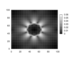
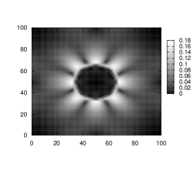
Figure 4: Spurious contributions around a static $2d$ drop for different density ratios with the standard SC model (6) and (7). Left: we show the local Mach number defined as $\sqrt{u^{2}_{x}+u^{2}_{y}}/c_{s}$ with $c_{s}$ the lattice sound speed. A drop of radius $15\Delta x$ and density ratio $\Delta\rho/\rho_{g}\sim 35$, obtained with ${\cal G}_{b}=-6.0$ in (6), is considered. Right: the same as in the case of left figure with a higher density ratio $\Delta\rho/\rho_{g}\sim 60$ obtained with ${\cal G}_{b}=-7.0$ in (6). Note in both plots the angular dependency due to lack of perfect radial symmetry in the forcing terms. In all numerical cases the lattice Boltzmann equation (1) has been integrated in time in a fully periodic $2d$ domain $L_{x}\times L_{y}=100\Delta x\times 100\Delta x$ with the drop put in the middle of the system. The relaxation time is $\tau=1.0\Delta t$.

where ${\bm{e}}_{x}=(1,0)$ and ${\bm{e}}_{y}=(0,1)$ are unit vectors in Cartesian coordinates. If we have axial symmetry of the density distribution we must have: $\psi=\psi(r)$. Because of ${\bm{\nabla}}={\bm{e}}_{r}\partial r$ and $\nabla^{2}=\partial_{r}^{2}+r^{-1}\partial_{r}$ for an axially symmetric function, the first term in the rhs of (27) is isotropic. On the other hand, the $2$nd and $3$rd terms, that arise only at the fifth order, are manifestly anisotropic. We should also notice that in the previous section, we limited our analytical analysis to the 4th order expansion, and all the numerical comparison where made by checking that spurious currents arising from higher orders were negligible, since we chose a stationary regime with small local gradients in the density field. Nevertheless, on the route to higher density ratios, i.e. for cases with high local density gradients, one necessarily meets with the problem of anisotropic contributions. In figure (4) we show the structure of the spurious currents for two cases. As one can see, the currents exhibit typical anisotropies with a quadrupolar modulation, the result of anisotropies induced by higher order derivatives in the pseudo-potential expansion (27) and they are enhanced systematically when the density separation between the two phases is increased.

To further support the previous statement, we have solved the Laplace equation, $\Delta{\bm{u}}=0$ with anisotropic boundary conditions on a ring, $u_{r}=cos(4\theta)$,$u_{\theta}=0$ for $r_{1}<r<r_{2}$ (see caption of figure (5) for details). The result is a non-zero profile in the bulk regions. This is also compared qualitatively with the spurious currents picture from a stationary state of a numerical simulation and a good qualitative agreement is observed (see figure (5)). From these pictures, we see that spurious currents, once generated on the interface, spread through the bulk regions, thereby corrupting the physical content of numerical simulations.

Having assessed that spurious currents are triggered by high-order angular harmonics due to lack of sufficient isotropy, it is natural to seek new models with a higher degree of isotropy. There are at least two parallel ways to remove this problem. Either one improves the support of the underlying lattice structure coupled by the pseudo-potential terms, so as to push anisotropy to higher and higher Taylor orders, or one can keep a given degree of isotropy of the forcing term and improved grid resolution, so that curved surfaces become more and more refined, hence subject to smaller local density gradients.

III.1 Isotropy at a fixed discretization

The former kind of technical improvement has already been proposed by Shan . Here we support these previous findings, and we extend them systematically to higher orders in full details for both $2d$ and $3d$ cases (see Appendixes C and D). Following Wolfram , the key idea consists of enlarging only the set of spatial grid points coupled by the pseudo-potential $\psi$ and choosing the appropriate weights to enforce isotropy up to the desired order. For any practical purpose, one writes

$$F_{i}=-{\cal G}_{b}c^{2}_{s}\psi({\bm{x}})\sum_{l}w(|{\bm{c}}_{l}|^{2})\psi({\bm{x}}+{\bm{c}}_{l})c_{l}^{i}$$ (28)

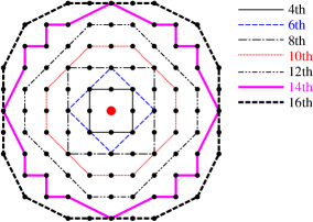
Figure 6: The grid points identifying the set of velocity fields for a $2d$ case. With reference to the weights reported in table 1, different degrees of isotropy can be achieved: 4th order (up to $w(2)$), 6th order (up to $w(4)$), 8th order (up to $w(8)$), 10th order (up to $w(10)$), 12th order (up to $w(17)$), 14th order (up to $w(25)$) and 16th order (up to $w(32)$).

where ${\bm{c}}_{l}$ runs over a given set of grid points, changing according to the required order of isotropy (see figure (6)) . In fact, by applying the Taylor expansion (all details in appendix C) to (28), one obtains:

$$\begin{split}F_{i}=-{\cal G}_{b}c_{s}^{2}\psi({\bm{x}})\Biggl{[}E^{(2)}_{ij}\partial_{j}\psi+\frac{1}{3!}E^{(4)}_{ijkl}\partial_{jkl}\psi+\frac{1}{5!}E^{(6)}_{ijklpq}\partial_{jklpq}\psi+\frac{1}{7!}E^{(8)}_{ijklpqst}\partial_{jklpqst}\psi+..\Biggr{]},\end{split}$$ (29)

with

$$E^{(m)}=E^{(m)}_{i_{1}i_{2}...i_{m}}=\sum_{l}w(|{\bm{c}}_{l}|^{2}){\bm{c}}^{i_{1}}_{l}{\bm{c}}^{i_{2}}_{l}...{\bm{c}}^{i_{m}}_{l}$$ (30)

and (obviously) zero odd tensors:

$$E^{(2n+1)}=0.$$ (31)

The weights can be chosen in such a way to recover isotropy to the desired order (see appendixes C and D). Clearly, more velocities are needed in the implementation of the forcing terms (see figure (6)). Numerical results (see figure (7)) do confirm a decay of the magnitude of the spurious contributions as the order of isotropy is raised. Although the practical implementation of higher-order scheme might not be as straightforward as the standard SC case, it is nonetheless reassuring to know that a well-defined procedure to tame spurious currents is available.

III.2 Refinement at a fixed degree of isotropy

Since non-isotropic terms in the standard SC forcing scale with fifth-order derivatives, it is plausible to expect that these terms can be attenuated also by a refinement of the interface resolution, i.e. by the rescaling procedure previously illustrated. In fact, in the standard formulation (27) the spurious contributions are induced by the terms ${\bm{e}}_{x}\frac{\partial_{x}^{5}\psi}{180}$ and ${\bm{e}}_{y}\frac{\partial_{y}^{5}\psi}{180}$ that should fade away by a progressive refinement of the grid.

In figure (8) we show how refining the grid for a fixed surface tension does indeed decrease the amplitude of spurious velocities. Using (15) and (20), with the scaling $A_{2}\sim 1/\rho^{2}_{0}$, the macroscopic system stays the same: same surface tension and same density ratio. The only difference is a net reduction of the spurious velocity. Let us notice that the improvement due to grid-refinement within the extended pseudo-potential (14) with pressure tensor (15) seems more effective than the one induced by high-order isotropic forcing in the original SC model. Indeed, comparing figure (7) and (8) one notices that in the latter an almost complete depletion of spurious currents is obtained already with a simple factor $2$ in the rescaled coordinate. On the other hand, to reach similar level of accuracy in the original SC model one needs to improve the isotropy of the forcing up to order $10$ or even more.
The fact that the smoothing of the density profile permits to reduce considerably spurious contributions allows to achieve quite large density ratios, up to the order of $\Delta\rho/\rho_{g}\sim 100$, as shown in figure (9), where we plot the maximal spurious velocity $|U|_{max}$ normalized to the sound speed as a function of the density ratio.
Of course, one may also imagine to combine the two proposals, using the extended formulation (14) with higher degrees of isotropy. Whether the numerical effort is worthwhile has to be decided on a case-by-case basis.

IV CONCLUSIONS

The SC model is one of the most successful spinoffs of lattice Boltzmann theory. It has nonetheless made the object of extensive criticism over the last decade Joseph . Part of this criticism is simply misplaced, some other is not. In particular, lack of thermodynamic consistency, surface tension tied-down to the equation of state, and spurious currents near sharp interfaces, have spurred doubts on the applicability of the SC method to the simulation of realistic multi-phase flows. In this paper we have elucidated the physical reasons behind the above weaknesses, and also suggested practical ways around them in the large-scale limit.

First, we have shown that by enlarging the number of coupling terms in the pseudo-potential expression, one can push the method at varying the density ratios and the surface tensions independently and over a wide range of parameters. The main limitation in achieving a systematic enhancement of density ratios is due to spurious currents in static curved interfaces. This limits both numerical stability in the dynamical evolution and the intimately physical correctness even for the static case.

Second, we have shown how to overcome this problem by developing improved versions of pseudo-potential interactions. The goal is to reduce anisotropy contributions that are the source of spurious currents. We achieved this systematically, either by a refinement of the curved interface, so as to soften the local density gradients, or by improving the isotropy of the discretized pseudo-potential. The first method is more effective, leading to a numerical reduction of the maximal current up to a factor $10$ with only a doubling in the grid resolution. We have shown that this stretching of the interface can be achieved by a simple rescaling of the coupling strengths with the reference density of the pseudopotential. This permits to achieve an ’adaptive’ form of local grid refinement without changing the structure of the lattice nodes.

The present analysis has been carried out for a given choice of the pseudopotential $\psi(\rho)$. In principle, the major conclusions should carry over to other, possibly more effective, functional forms of $\psi$ Yuan .

Besides clarifying the theoretical foundations of the original SC model, it is hoped that the extended version presented in this work will help setting the stage for future and more challenging applications of pseudo-potential methods to the simulation of complex multiphase flows.

V Appendix A

In this appendix we discuss the tensorial structures that lead to a vector structure of the form

$$J_{i}=\frac{1}{2}\psi\partial_{i}\Delta\psi=\frac{1}{2}\psi\partial_{ill}\psi$$ (32)

where doubled indexes are summed upon. We start from the most general expression for a second order, non diagonal tensor involving derivatives only in the second order:

$$S_{ij}=\left[\frac{c}{2}(\partial_{l}\psi)(\partial_{l}\psi)+d\psi\partial_{ll}\psi\right]\delta_{ij}+a(\partial_{i}\psi)(\partial_{j}\psi)+b\psi\partial_{ij}\psi$$ (33)

where $a,b,c,d$ are meant to be fixed upon consistency with expression (32). It is infact verified that upon differentiation:

$$\partial_{j}S_{ij}=c\partial_{j}\psi\partial_{ij}\psi+d\partial_{i}\psi\partial_{jj}\psi+d\psi\partial_{ijj}\psi+a\partial_{ij}\psi\partial_{j}\psi+a\partial_{i}\psi\partial_{jj}\psi+b\partial_{j}\psi\partial_{ij}\psi+b\psi\partial_{ijj}\psi.$$ (34)

To be consistent with the expression of the forcing we must impose:

$$\left\{\begin{array}[]{l}a+b+c=0\\ a+d=0\\ d+b=\frac{1}{2}\\ \end{array}\right.$$ (35)

and we end up with three constraints and four constants. This means that there are infinitely many choices of $S_{ij}$ satisfying the condition:

$$\partial_{j}S_{ij}=J_{i}$$ (36)

and we need another constraint to close the problem and give unambiguously our tensor. Even if the tensor structure is not uniquely determined, when we apply our arguments to the case of a flat interface whose dishomogeneities develop along a $y$ coordinate, we notice that the normal component of the above tensor is:

$$S_{yy}=\frac{1}{2}\psi\partial_{yy}\psi+\left(a+\frac{c}{2}\right)(\partial_{y}\psi)^{2}$$ (37)

and from the last $2$ expressions of (35) we obtain $a-b=-\frac{1}{2}$ that used in the first one imposes:

$$2a+c=-\frac{1}{2}\Rightarrow a+\frac{c}{2}=-\frac{1}{4}.$$ (38)

So, even if the tensor is not uniquely determined, its normal component is uniquely given by

$$S_{yy}=\frac{1}{2}\psi\partial_{yy}\psi-\frac{1}{4}(\partial_{y}\psi)^{2}.$$ (39)

This implies that when using a mechanical stability equation (11) with a fixed boundary condition we are able to extract the same profile as a function of $y$. Then, from the expression (33) we can also write the equivalent of the surface tension considering the mismatch between the normal $S_{yy}$ and tangential components $S_{xx}$ :

$$\sigma=\displaystyle\int_{-\infty}^{+\infty}(a(\partial_{y}\psi)^{2}+b\psi\partial_{yy}\psi)=(a-b)\int_{-\infty}^{+\infty}(\partial_{y}\psi)^{2}.$$ (40)

Again, from that the last two expression of (35) we get $a-b=-\frac{1}{2}$. This means that the surface tension is uniquely determined.

VI Appendix B

In this appendix we show how to derive non isotropic contributions from discretizations. The forcing term is written in the form

$$F_{i}=-{\cal G}_{b}c^{2}_{s}\psi({\bm{x}})\sum_{l}w(|{\bm{c}}_{l}|^{2})\psi({\bm{x}}+{\bm{c}}_{l}){c}_{l}^{i}.$$ (41)

Applying the Taylor expansion, one obtains

$$\begin{split}F_{i}=-{\cal G}_{b}c^{2}_{s}\psi({\bm{x}})\Biggl{[}E^{(2)}_{ij}\partial_{j}\psi+\frac{1}{3!}E^{(4)}_{ijkl}\partial_{jkl}\psi+\frac{1}{5!}E^{(6)}_{ijklpq}\partial_{jklpq}\psi+\frac{1}{7!}E^{(8)}_{ijklpqst}\partial_{jklpqst}\psi+..\Biggr{]},\end{split}$$ (42)

with

$$E^{(m)}=E^{(m)}_{i_{1}i_{2}...i_{m}}=\sum_{l}w(|{\bm{c}}_{l}|^{2}){c}^{i_{1}}_{l}{c}^{i_{2}}_{l}...{c}^{i_{m}}_{l}.$$ (43)

and (obviously) zero odd tensors:

$$E^{(2n+1)}=0.$$ (44)

The even tensors are written as

$$E_{i_{1}i_{2}...i_{2n}}^{(2n)}={\cal C}^{(2n)}\Delta_{i_{1}i_{2}...i_{2n}}^{(2n)},$$ (45)

where $\Delta^{(2n)}$ is given by the recursion relation Wolfram

$$\Delta_{ij}^{(2)}=\delta_{ij},\ \ \ \Delta_{ijkl}^{(4)}=\delta_{ij}\delta_{kl}+\delta_{ik}\delta_{jl}+\delta_{il}\delta_{jk},$$

$$\Delta_{i_{1}i_{2}...i_{2n}}^{(2n)}=\sum_{j=2}^{2n}\delta_{i_{1}i_{j}}\Delta_{i_{2}i_{3}...i_{j-1}i_{j+1}...i_{2n}}^{(2n-2)}.$$ (46)

In our mean field approach, $\psi$ is a function of the density. If the density distribution is axially symmetric, $\psi$ is also axially symmetric, $\psi=\psi(r)$. Then, the force $F_{i}$ should be written as

$$F_{i}({\bm{x}})=\frac{x_{i}}{r}\tilde{F}(r),$$ (47)

where $\tilde{F}$ is a scalar function. It should be noted that the isotropy (45) for all ${\bm{E}}^{(2n)}$ is essential in order to satisfy the relation (47). Now, we will show that the truncated isotropy induces the anisotropic force, which triggers the spurious currents, even when the density distribution is axially symmetric. Let us consider the standard case of $2DQ9$. As already noticed in the text, this is a $4$th-order approximation in the isotropy and the weights are given by

$$w(1)=1/3,\ \ w(2)=1/12,$$

$$w(n)=0\ \ \ {\rm for}\ \ \ n\geq 3.$$ (48)

This approximation means that all the tensors up to the $4$th-order (${\bm{E}}^{(2)}$ and ${\bm{E}}^{(4)}$) are isotropic but the higher order ones ${\bm{E}}^{(n)}$ ($n\geq 6$) are not. Using standard Taylor expansion for lattice Boltzmann populations one obtains after some lengthly algebra:

$$\begin{split}\sum_{l}w(|{\bm{c}}_{l}|^{2})\psi({\bm{x}}+{\bm{c}}_{l})c_{l}^{x}=&\partial_{x}\psi+\frac{1}{6}\partial_{x}(\partial_{x}^{2}+\partial_{y}^{2})\psi+\partial_{x}\left(\frac{1}{120}\partial_{x}^{4}+\frac{1}{36}\partial_{x}^{2}\partial_{y}^{2}+\frac{1}{72}\partial_{y}^{4}\right)\psi+...,\\ \sum_{l}w(|{\bm{c}}_{l}|^{2})\psi({\bm{x}}+{\bm{c}}_{l})c_{l}^{y}=&\partial_{y}\psi+\frac{1}{6}\partial_{y}(\partial_{x}^{2}+\partial_{y}^{2})\psi+\partial_{y}\left(\frac{1}{72}\partial_{x}^{4}+\frac{1}{36}\partial_{x}^{2}\partial_{y}^{2}+\frac{1}{120}\partial_{y}^{4}\right)\psi+...\end{split}$$ (49)

Using a nabla operator, (49) is rewritten as

$$\sum_{l}w(|{\bm{c}}_{l}|^{2})\psi({\bm{x}}+{\bm{c}}_{l}){\bm{c}}_{l}={\bm{\nabla}}\left(1+\frac{1}{6}\nabla^{2}+\frac{1}{72}\nabla^{2}\nabla^{2}\right)\psi+{\bm{e}}_{x}\frac{\partial_{x}^{5}\psi}{180}+{\bm{e}}_{y}\frac{\partial_{y}^{5}\psi}{180}+{\cal O}(\partial^{7}),$$ (50)

where ${\bm{e}}_{x}=(1,0)$ and ${\bm{e}}_{y}=(0,1)$ are unit vectors in Cartesian coordinates. Next we assume axial symmetry of the density distribution, i.e., $\psi=\psi(r)$. Because of ${\bm{\nabla}}={\bm{e}}_{r}\partial r$ and $\nabla^{2}=\partial_{r}^{2}+r^{-1}\partial_{r}$ for an axially symmetric function, the 1st term in the r.h.s of (50) is isotropic. On the other hand, the 2nd and 3rd terms, related to the anisotropic tensor ${\bm{E}}^{(6)}$ in (42), are not. Now the force $F_{i}$ is decomposed into the isotropic and anisotropic parts, i.e.,

$$F_{i}({\bm{x}})=\frac{x_{i}}{r}\tilde{F}(r)+F_{i}^{\prime}({\bm{x}}).$$ (51)

Within the $O(\partial^{5})$ approximation, $\tilde{F}(r)$ and $F_{i}^{\prime}({\bm{x}})$ are respectively given by

$$\tilde{F}(r)=-{\cal G}_{b}c_{s}^{2}\psi\partial_{r}\Biggl{(}1+\frac{1}{6r}\frac{{\rm d}}{{\rm d}r}r\frac{{\rm d}}{{\rm d}r}+\frac{1}{72r}\frac{{\rm d}}{{\rm d}r}r\frac{{\rm d}}{{\rm d}r}r^{-1}\frac{{\rm d}}{{\rm d}r}r\frac{{\rm d}}{{\rm d}r}\Biggr{)}\psi,$$ (52)

$$F_{1}^{\prime}=-\frac{{\cal G}_{b}c_{s}^{2}\psi\partial_{x}^{5}\psi}{180},\ \ \ F_{2}^{\prime}=-\frac{{\cal G}_{b}c_{s}^{2}\psi\partial_{y}^{5}\psi}{180}.$$ (53)

The anisotropic force $F_{i}^{\prime}$ due to the anisotropy of ${\bm{E}}^{(6)}$ is responsible for the spurious currents. Higher orders can be computed similarly (for the interested reader please contact the authors).

VII Appendix C

Here we detail the exact procedures leading to higher order isotropic terms in the forcing contribution for a regular lattice in $2d$. The velocity phase space and forcing weights for isotropic terms up to $16$th order are explicitly given in figure (6). To treat correctly isotropy from a lattice set of velocity vectors (${c}^{i}_{l},i=x,y$) the starting point is the $2$ point tensor on the lattice which is assumed normalized to unity

$$\sum_{l}{c}_{l}^{i}{c}_{l}^{j}w(|{\bm{c}}_{l}|^{2})=\delta_{ij}.$$ (54)

Considering the regular structure of the lattice and the consequent symmetry of $c_{l}^{i}$ with respect to $i=x$ and $i=y$, one can write (54) in the simplified form

$$\sum_{l}(c_{l}^{x})^{2}w(|{\bm{c}}_{l}|^{2})=1.$$ (55)

The fourth-order isotropy is imposed by

$$\sum_{l}{c}_{l}^{i}{c}_{l}^{j}{c}_{l}^{j}{c}_{l}^{s}w(|{\bm{c}}_{l}|^{2})={\cal C}^{(4)}\left(\delta_{ij}\delta_{ks}+\delta_{ik}\delta_{js}+\delta_{is}\delta_{jk}\right),$$ (56)

where ${\cal C}^{(4)}$ is a constant. Since one obtains

$$\sum_{l}({c}_{l}^{x})^{4}w(|{\bm{c}}|^{2}_{l})=3{\cal C}^{(4)},\ \ \ \sum_{l}({c}_{l}^{x})^{2}({c}_{l}^{y})^{2}w(|{\bm{c}}_{l}|^{2})={\cal C}^{(4)},$$

a condition to satisfy (56) is written as

$$\frac{\sum_{l}({c}_{l}^{x})^{4}w(|{\bm{c}}_{l}|^{2})}{\sum_{l}({c}_{l}^{x})^{2}({c}_{l}^{y})^{2}w(|{\bm{c}}_{l}|^{2})}=3.$$ (57)

In terms of lattice vector this can be achieved with the standard $2DQ9$ model with weights $w(1)=1/3$ and $w(2)=1/12$ and the corresponding lattice velocities:
$w(1)$:

$$({\bm{c}}_{1}\ {\bm{c}}_{2}\ {\bm{c}}_{3}\ {\bm{c}}_{4})=\left(\begin{array}[]{rrrr}1&0&-1&0\\ 0&1&0&-1\\ \end{array}\right),$$ (58)

$w(2)$:

$$({\bm{c}}_{5}\ {\bm{c}}_{6}\ {\bm{c}}_{7}\ {\bm{c}}_{8})=\left(\begin{array}[]{rrrr}1&-1&-1&1\\ 1&1&-1&-1\\ \end{array}\right).$$ (59)

More general conditions can then be obtained for higher order tensors. For example, the $6$th, $8$th, $10$th and $12$th-order isotropies are given by

$$\begin{split}\sum_{l}{c}_{l}^{i_{1}}{c}_{l}^{i_{2}}{c}_{l}^{i_{3}}{c}_{l}^{i_{4}}{c}_{l}^{i_{5}}{c}_{l}^{i_{6}}w(|{\bm{c}}_{l}|^{2})=&{\cal C}^{(6)}\left(\delta_{i_{1}i_{2}}\delta_{i_{3}i_{4}}\delta_{i_{5}i_{6}}+..\right),\\ \sum_{l}{c}_{l}^{i_{1}}{c}_{l}^{i_{2}}{c}_{l}^{i_{3}}{c}_{l}^{i_{4}}{c}_{l}^{i_{5}}{c}_{l}^{i_{6}}{c}_{l}^{i_{7}}{c}_{l}^{i_{8}}w(|{\bm{c}}_{l}|^{2})=&{\cal C}^{(8)}\left(\delta_{i_{1}i_{2}}\delta_{i_{3}i_{4}}\delta_{i_{5}i_{6}}\delta_{i_{7}i_{8}}+..\right),\\ \sum_{l}{c}_{l}^{i_{1}}{c}_{l}^{i_{2}}{c}_{l}^{i_{3}}{c}_{l}^{i_{4}}{c}_{l}^{i_{5}}{c}_{l}^{i_{6}}{c}_{l}^{i_{7}}{c}_{l}^{i_{8}}{c}_{l}^{i_{9}}{c}_{l}^{i_{10}}w(|{\bm{c}}_{l}|^{2})=&{\cal C}^{(10)}\left(\delta_{i_{1}i_{2}}\delta_{i_{3}i_{4}}\delta_{i_{5}i_{6}}\delta_{i_{7}i_{8}}\delta_{i_{9}i_{10}}+..\right),\\ \sum_{l}{c}_{l}^{i_{1}}{c}_{l}^{i_{2}}{c}_{l}^{i_{3}}{c}_{l}^{i_{4}}{c}_{l}^{i_{5}}{c}_{l}^{i_{6}}{c}_{l}^{i_{7}}{c}_{l}^{i_{8}}{c}_{l}^{i_{9}}{c}_{l}^{i_{10}}{c}_{l}^{i_{11}}{c}_{l}^{i_{12}}w(|{\bm{c}}_{l}|^{2})=&{\cal C}^{(12)}\left(\delta_{i_{1}i_{2}}\delta_{i_{3}i_{4}}\delta_{i_{5}i_{6}}\delta_{i_{7}i_{8}}\delta_{i_{9}i_{10}}\delta_{i_{11}i_{12}}+..\right).\end{split}$$ (60)

And the mixed contributions can be constructed as well:

$$\sum_{l}({c}_{l}^{x})^{2n}({c}_{l}^{y})^{2m}w(|{\bm{c}}_{l}|^{2})={\cal C}^{(2n+2m)}(2n-1)!!(2m-1)!!,$$ (61)

where $(2n-1)!!=(2n-1)\times(2n-3)\times...\times 1$. Then, to achieve isotropy at higher orders one should introduce some requirements on the tensors. Just to give an example, for the isotropy up to the $6$th order one should require that:

$$\frac{\sum_{l}({c}_{l}^{x})^{4}w(|{\bm{c}}_{l}|^{2})}{\sum_{l}({c}_{l}^{x})^{2}({c}_{l}^{y})^{2}w(|{\bm{c}}_{l}|^{2})}=3$$ (62)

$$\frac{\sum_{l}({c}_{l}^{x})^{6}w(|{\bm{c}}_{l}|^{2})}{\sum_{l}({c}_{l}^{x})^{4}({c}_{l}^{y})^{2}w(|{\bm{c}}_{l}|^{2})}=5.$$ (63)

these translate to the matrix relation

$$\left(\begin{array}[]{rrr}2&4&8\\ 1&-4&16\\ 1&-8&64\\ \end{array}\right)\left(\begin{array}[]{l}w(1)\\ w(2)\\ w(4)\\ \end{array}\right)=\left(\begin{array}[]{l}1\\ 0\\ 0\\ \end{array}\right)$$ (64)

that can be satisfied using $12$ velocities with weights $w(1)=4/15,w(2)=1/10$ and $w(4)=1/120$

$w(1)$:

$$({\bm{c}}_{1}\ {\bm{c}}_{2}\ {\bm{c}}_{3}\ {\bm{c}}_{4})=\left(\begin{array}[]{rrrr}1&0&-1&0\\ 0&1&0&-1\\ \end{array}\right),$$ (65)

$w(2)$:

$$({\bm{c}}_{5}\ {\bm{c}}_{6}\ {\bm{c}}_{7}\ {\bm{c}}_{8})=\left(\begin{array}[]{rrrr}1&-1&-1&1\\ 1&1&-1&-1\\ \end{array}\right),$$ (66)

$w(4)$:

$$({\bm{c}}_{9}\ {\bm{c}}_{10}\ {\bm{c}}_{11}\ {\bm{c}}_{12})=\left(\begin{array}[]{rrrr}2&0&-2&0\\ 0&2&0&-2\\ \end{array}\right).$$ (67)

Higher order calculations are lengthly and not reported here. The set of vectors can be extracted from figure (6) while the weights can be found in table 1.

VIII Appendix D

The same calculations are then arranged in $3d$. For each $w(n)$ (reported in table 2), the corresponding velocity vectors ${\bm{c}}_{l}$ are shown below:

$w(1)$:

$$({\bm{c}}_{1}\ {\bm{c}}_{2}\ {\bm{c}}_{3}\ {\bm{c}}_{4}\ {\bm{c}}_{5}\ {\bm{c}}_{6})=\left(\begin{array}[]{rrrrrrrr}1&-1&0&0&0&0\\ 0&0&1&-1&0&0\\ 0&0&0&0&1&-1\\ \end{array}\right),$$ (68)

$w(2)$:

$$\begin{split}&({\bm{c}}_{7}\ {\bm{c}}_{8}\ {\bm{c}}_{9}\ {\bm{c}}_{10}\ {\bm{c}}_{11}\ {\bm{c}}_{12}\ {\bm{c}}_{13}\ {\bm{c}}_{14}\ {\bm{c}}_{15}\ {\bm{c}}_{16}\ {\bm{c}}_{17}\ {\bm{c}}_{18})\\ =&\left(\begin{array}[]{rrrrrrrrrrrrrrrr}1&1&-1&-1&1&1&-1&-1&0&0&0&0\\ 1&-1&1&-1&0&0&0&0&1&1&-1&-1\\ 0&0&0&0&1&-1&1&-1&1&-1&1&-1\\ \end{array}\right),\end{split}$$ (69)

$w(3)$:

$$({\bm{c}}_{19}\ {\bm{c}}_{10}\ {\bm{c}}_{21}\ {\bm{c}}_{22}\ {\bm{c}}_{23}\ {\bm{c}}_{24}\ {\bm{c}}_{25}\ {\bm{c}}_{26})=\left(\begin{array}[]{rrrrrrrrrr}1&1&1&1&-1&-1&-1&-1\\ 1&1&-1&-1&1&1&-1&-1\\ 1&-1&1&-1&1&1&-1&-1\\ \end{array}\right),$$ (70)

$w(4)$:

$$({\bm{c}}_{27}\ {\bm{c}}_{28}\ {\bm{c}}_{29}\ {\bm{c}}_{30}\ {\bm{c}}_{31}\ {\bm{c}}_{32})=\left(\begin{array}[]{rrrrrrrr}2&-2&0&0&0&0\\ 0&0&2&-2&0&0\\ 0&0&0&0&2&-2\\ \end{array}\right),$$ (71)

$w(5)$:

$$\begin{split}&({\bm{c}}_{33}\ {\bm{c}}_{34}\ {\bm{c}}_{35}\ {\bm{c}}_{36}\ {\bm{c}}_{37}\ {\bm{c}}_{38}\ {\bm{c}}_{39}\ {\bm{c}}_{40}\ {\bm{c}}_{41}\ {\bm{c}}_{42}\ {\bm{c}}_{43}\ {\bm{c}}_{44}\\ &{\bm{c}}_{45}\ {\bm{c}}_{46}\ {\bm{c}}_{47}\ {\bm{c}}_{48}\ {\bm{c}}_{49}\ {\bm{c}}_{50}\ {\bm{c}}_{51}\ {\bm{c}}_{52}\ {\bm{c}}_{53}\ {\bm{c}}_{54}\ {\bm{c}}_{55}\ {\bm{c}}_{56})\\ =&\left(\begin{array}[]{rrrrrrrrrrrr}2&2&-2&-2&2&2&-2&-2&1&-1&1&-1\\ 1&-1&1&-1&0&0&0&0&2&2&-2&-2\\ 0&0&0&0&1&-1&1&-1&0&0&0&0\\ \end{array}\right.\\ &\left.\begin{array}[]{rrrrrrrrrrrr}0&0&0&0&1&-1&1&-1&0&0&0&0\\ 2&2&-2&-2&0&0&0&0&1&-1&1&-1\\ 1&-1&1&-1&2&2&-2&-2&2&2&-2&-2\\ \end{array}\right),\end{split}$$ (72)

$w(6)$:

$$({\bm{c}}_{57}\ ..\ {\bm{c}}_{80})=\left(\begin{array}[]{rrr}2&...&-1\\ 1&...&-1\\ 1&...&-2\\ \end{array}\right),$$ (73)

$w(8)$:

$$({\bm{c}}_{81}\ ..\ {\bm{c}}_{92})=\left(\begin{array}[]{rrr}2&...&0\\ 2&...&-2\\ 0&...&-2\\ \end{array}\right),$$ (74)

$w_{221}(9)$:

$$({\bm{c}}_{93}\ ..\ {\bm{c}}_{116})=\left(\begin{array}[]{rrr}2&...&-1\\ 2&...&-2\\ 1&...&-2\\ \end{array}\right),$$ (75)

$w_{300}(9)$:

$$({\bm{c}}_{117}\ ..\ {\bm{c}}_{122})=\left(\begin{array}[]{rrr}3&...&0\\ 0&...&0\\ 0&...&-3\\ \end{array}\right),$$ (76)

$w(10)$:

$$({\bm{c}}_{123}\ ..\ {\bm{c}}_{146})=\left(\begin{array}[]{rrr}3&...&0\\ 1&...&-1\\ 0&...&-3\\ \end{array}\right),$$ (77)

$w(11)$:

$$({\bm{c}}_{147}\ ..\ {\bm{c}}_{170})=\left(\begin{array}[]{rrr}3&...&-1\\ 1&...&-1\\ 1&...&-3\\ \end{array}\right).$$ (78)

Figure 1: Smoothing of interface properties. We show the static profiles for a flat interface with an improved SC model (14) and (7). The parameters are chosen to produce a macroscopic pressure tensor (15) keeping fixed $A_{1}=-5.0$ (same density ratio) and at varying $A_{2}$: $A_{2}=-5.0$ ($\Box$) and $A_{2}=-30.0$ ($\circ$). The results of numerical simulations are compared with the analytical estimates (solid lines) obtained solving the mechanical stability equation (11) applied to (15). Notice the smoothing in the interface for a fixed density ratio due to a change in the surface tension. In all numerical cases the lattice Boltzmann equation (1) has been integrated in time in a fully periodic domain $L_{x}\times L_{y}=100\Delta x\times 100\Delta x$ with a flat strip of liquid in an otherwise gaseous domain. The relaxation time is $\tau=0.7\Delta t$.

Figure 2: Laplace test for the same density ratio obtained from the numerical simulation of the improved SC model (14) and (7). The parameters are chosen to reproduce a macroscopic pressure tensor (15) with $A_{1}=-5.0$ and different $A_{2}$: $A_{2}=-5.0$ ($\Box$), $A_{2}=-15.0$ ($\circ$), $A_{2}=-30.0$ ($\triangle$). For each case we plot the pressure drop $\Delta P$ as a function of the inverse radius of the static drop. Moreover we compare the results with the theoretical predictions (solid lines) given by the continuum analysis that leads to $\sigma(A_{2}={-5})=0.0398$, $\sigma(A_{2}={-15})=0.0716$ and $\sigma(A_{2}={-30})=0.100$ in lattice units. Numerical details are the same of figure (1) with the only difference that now we use a drop in the middle of the domain.

Figure 3: Smoothing of interface properties. We show the static profiles for a flat interface with an improved SC model (14) and (20). The parameters are chosen such as to produce a macroscopic pressure tensor (21) with $A_{1}=-5.0$ and $A_{2}=-5.0/\rho^{2}_{0}$ for different values of $\rho_{0}$: $\rho_{0}=1.0$ ($\Box$), $\rho_{0}=0.5$ ($\circ$) . Results are also compared with the analytical estimate resulting from our continuum interpretation (solid line). The two profiles have been plotted by rescaling the lattice grid by a factor $1/\rho_{0}$. Notice the increased interface grid resolution obtained at fixed density ratio. Inset: the results of the Laplace tests made on spherical droplets with the same density ratio and varying grid resolution is also plotted. Again, we get the same surface tension with different interface resolutions, $\rho_{0}=1.0$ ($\Box$), $\rho_{0}=0.7$ ($\circ$), $\rho_{0}=0.5$ ($\triangle$). In all numerical cases the lattice Boltzmann equation has been integrated in time in a fully periodic domain $L_{x}\times L_{y}=100\Delta x\times 100\Delta x$ with a flat strip of liquid in an otherwise gaseous domain. The relaxation time is $\tau=0.7\Delta t$.

Figure 5: Spurious contributions in Lattice Boltzmann and their continuum interpretation. Left: we report the structure of the velocity field around a static drop of radius $15\Delta x$ and density ratio $\Delta\rho/\rho_{g}\sim 50$. The data are the same of right panel of figure (4). Right: for a qualitative comparison we have solved the Laplace equation together with the continuity equations with a matching condition in a radial ring of a given width. The velocity field is obtained in an iterative way by first solving the Poisson equation $\nabla^{2}\phi=\nabla\cdot{\bm{u}}$ and then renewing the velocity filed as ${\bm{u}}\rightarrow{\bm{u}}-\nabla\phi$. For both ${\bm{u}}$ and $\phi$ periodic boundary conditions are imposed in the horizontal and vertical directions. On the ring of range $17.5\Delta x<r<20.5\Delta x$ the matching condition: $u_{r}=\mbox{cos}4\theta,u_{\theta}=0$ is imposed being $u_{r}$ and $u_{\theta}$ the radial and azimuthal components of the velocity field respectively.

Figure 7: Reduction of spurious currents with higher order isotropic tensors in the forcing terms. The spurious contributions for a static drop are analyzed for a density ratio $\Delta\rho/\rho_{g}\sim 50$ obtained for a standard SC model (6) and (7). The parameter chosen is ${\cal G}_{b}=-7.0$. We show the vertical velocity, $u_{y}$, normalized with the lattice speed of sound, $c_{s}$, at $x=L_{x}/2$ and as a function of $y/\Delta x$. The different plots correspond to different degrees of isotropy in the forcing term (6): $4$th order ($\Box$), $6$th order ($\circ$), $8$th order ($\triangle$) and $10$th order ($\times$). Notice the reduction of the spurious contributions in the proximity of the droplet surface, $y/\Delta x\sim 30,70$. Data are obtained from Lattice Boltzmann equation (1) in a fully periodic domain $L_{x}\times L_{y}=100\Delta x\times 100\Delta x$ and $\tau=1.0\Delta t$ in lattice units.

Figure 8: reduction of the spurious currents with grid refinement at changing $\rho_{0}$. The spurious contributions for a static drop are analyzed for a density ratio $\Delta\rho/\rho_{g}\sim 50$ obtained for the improved SC model (14) and (20). The parameters are chosen in such a way to reproduce (15) with $A_{1}=-7.0$. We show the vertical velocity, $u_{y}$, normalized with the lattice speed of sound, $c_{s}$, at $x=L_{x}/2$ ad as a function of $y/\Delta x$. The different plots correspond to different degrees of refinement obtained with $A_{2}=-7.0/\rho^{2}_{0}$ in (15): $\rho_{0}=1.0$ ($\Box$), $\rho_{0}=0.75$ ($\circ$) and $\rho_{0}=0.5$ ($\triangle$). Details of the numerical simulations are the same of the previous figure.

Figure 9: Reduction of the spurious currents with refinement in the forcing terms. The spurious contributions for a static drop are analyzed for various density ratios obtained in the improved SC model (14) and (20). The parameters are chosen in such a way as to reproduce (15) with different $A_{1}$, thus changing the density ratio $\Delta\rho/\rho_{g}$. We show the maximum velocity due to spurious contributions, normalized with the lattice speed of sound ($c_{s}$) as a function of $\Delta\rho/\rho_{g}$. The $2$ different plots correspond to different degree of refinement obtained with $A_{2}=7.0/\rho^{2}_{0}$ in (21) and different values of $\rho_{0}$: $\rho_{0}=1.0$ ($\Box$), $\rho_{0}=0.5$ ($\circ$). Notice the net reduction of the spurious contributions at fixed macroscopic physics (same density ratio and surface tension) obtained through the rescaling $A_{2}\sim 1/\rho_{0}^{2}$. The numerical details are the same described in figure (8).

Table 1. Weights up to the 16th-order approximation for the case of $2d$ models. Notice that the weights for velocities with $|{\bm{c}}_{l}|^{2}=25$ needs to be chosen differently according to the directions in the $x-y$ plane. The notation $w_{x,y}(|{\bm{c}}_{l}|^{2})$ stands for the velocity lattice vectors $(\pm x_{1},\pm x_{2})$ and $(\pm x_{2},\pm x_{1})$.

	${\bm{E}}^{(6)}$	${\bm{E}}^{(8)}$	${\bm{E}}^{(10)}$	${\bm{E}}^{(12)}$	${\bm{E}}^{(14)}$	${\bm{E}}^{(16)}$
$w(1)$	$\displaystyle\frac{4}{15}$	$\displaystyle\frac{4}{21}$	$\displaystyle\frac{262}{1785}$	$\displaystyle\frac{68}{585}$	$\displaystyle\frac{19414}{228375}$	$\displaystyle\frac{285860656}{3979934595}$
$w(2)$	$\displaystyle\frac{1}{10}$	$\displaystyle\frac{4}{45}$	$\displaystyle\frac{93}{1190}$	$\displaystyle\frac{68}{1001}$	$\displaystyle\frac{549797}{10048500}$	$\displaystyle\frac{2113732952}{43779280545}$
$w(4)$	$\displaystyle\frac{1}{120}$	$\displaystyle\frac{1}{60}$	$\displaystyle\frac{7}{340}$	$\displaystyle\frac{1}{45}$	$\displaystyle\frac{175729}{7917000}$	$\displaystyle\frac{940787801}{43779280545}$
$w(5)$		$\displaystyle\frac{2}{315}$	$\displaystyle\frac{6}{595}$	$\displaystyle\frac{62}{5005}$	$\displaystyle\frac{50728}{3628625}$	$\displaystyle\frac{124525000}{8755856109}$
$w(8)$		$\displaystyle\frac{1}{5040}$	$\displaystyle\frac{9}{9520}$	$\displaystyle\frac{1}{520}$	$\displaystyle\frac{3029}{913500}$	$\displaystyle\frac{15841927}{3979934595}$
$w(9)$			$\displaystyle\frac{2}{5355}$	$\displaystyle\frac{4}{4095}$	$\displaystyle\frac{15181}{7536375}$	$\displaystyle\frac{2046152}{795986919}$
$w(10)$			$\displaystyle\frac{1}{7140}$	$\displaystyle\frac{2}{4095}$	$\displaystyle\frac{221}{182700}$	$\displaystyle\frac{14436304}{8755856109}$
$w(13)$				$\displaystyle\frac{2}{45045}$	$\displaystyle\frac{68}{279125}$	$\displaystyle\frac{18185828}{43779280545}$
$w(16)$				$\displaystyle\frac{1}{480480}$	$\displaystyle\frac{1139}{26796000}$	$\displaystyle\frac{13537939}{140093697744}$
$w(17)$				$0$	$\displaystyle\frac{68}{2968875}$	$\displaystyle\frac{231568}{3979934595}$
$w(18)$					$\displaystyle\frac{17}{1425060}$	$\displaystyle\frac{1516472}{43779280545}$
$w(20)$					$\displaystyle\frac{17}{5742000}$	$\displaystyle\frac{18769}{1591973838}$
$w_{50}(25)$					$\displaystyle\frac{1}{32657625}$	$\displaystyle\frac{184}{315867825}$
$w_{34}(25)$					$\displaystyle\frac{1}{32657625}$	$\displaystyle\frac{464}{795986919}$
$w(26)$						$\displaystyle\frac{1448}{4864364505}$
$w(29)$						$\displaystyle\frac{148}{4864364505}$
$w(32)$						$\displaystyle\frac{629}{400267707840}$

Table 2   Weights up to the 10th-order approximation for $3d$ models. Notice that the weights for velocities with $|{\bm{c}}_{l}|^{2}=9$ needs to be chosen differently according to the directions in the $x-y-z$ space. The notation $w_{x,y,z}(|{\bm{c}}_{l}|^{2})$ stands for the velocity lattice vectors $(\pm x_{1},\pm x_{2},\pm x_{3})$ plus permutation.

	$\displaystyle{\bm{E}}^{(6)}$	$\displaystyle{\bm{E}}^{(8)}$	$\displaystyle{\bm{E}}^{(10)}$
$w(1)$	$\displaystyle\frac{2}{15}$	$\displaystyle\frac{4}{45}$	$\displaystyle\frac{352}{5355}$
$w(2)$	$\displaystyle\frac{1}{15}$	$\displaystyle\frac{1}{21}$	$\displaystyle\frac{38}{1071}$
$w(3)$	$\displaystyle\frac{1}{60}$	$\displaystyle\frac{2}{105}$	$\displaystyle\frac{271}{14280}$
$w(4)$	$\displaystyle\frac{1}{120}$	$\displaystyle\frac{5}{504}$	$\displaystyle\frac{139}{14280}$
$w(5)$		$\displaystyle\frac{1}{315}$	$\displaystyle\frac{53}{10710}$
$w(6)$		$\displaystyle\frac{1}{630}$	$\displaystyle\frac{5}{2142}$
$w(8)$		$\displaystyle\frac{1}{5040}$	$\displaystyle\frac{41}{85680}$
$w_{221}(9)$			$\displaystyle\frac{1}{4284}$
$w_{300}(9)$			$\displaystyle\frac{1}{5355}$
$w(10)$			$\displaystyle\frac{1}{10710}$
$w(11)$			$\displaystyle\frac{1}{42840}$

References

• (1) R. Benzi, S. Succi & M. Vergassola,”The Lattice Boltzmann Equation: Theory and. Applications” Phys. Rep. 222, 145-197 (1992).
• (2) S. Chen and G. Doolen,”Lattice Boltzmann method for fluid flows” Annu. Rev. Fluid Mech. 30, 329-364 (1998).
• (3) D. Wolf-Gladrow, Lattice-Gas Cellular Automata And Lattice Boltzmann Models (Springer, New York, 2000)
• (4) M. R. Swift, W. R. Osborn, and J. M. Yeomans,” Lattice Boltzmann Simulation of Nonideal Fluids” Phys. Rev. Lett. 75, 830-833 (1995)
• (5) X. Shan and H. Chen,”Lattice Boltzmann model for simulating flows with multiple phases and components” Phys. Rev E 47, 1815 (1993).
• (6) X. Shan and H. Chen,” Simulation of nonideal gases and liquid-gas phase transitions by the lattice Boltzmann equation”Phys. Rev E 49, 2941 (1994).
• (7) T. M. Squires and S. R. Quake,”Microfluidics: Fluid physics at the nanoliter scale” Rev. Mod. Phys. 77, 977-1026 (2005).
• (8) P. Tabeling, Introduction a la microfluidique (Belin, Paris, 2003).
• (9) A. Dupuis and J. M. Yeomans,”Modelling Droplets on superhydrophobic surfaces: equilibrium states and transitions”, Langmuir 21, 2624-2629 (2005)
• (10) R. Benzi, L. Biferale, M. Sbragaglia, S. Succi, and F. Toschi ,”Mesoscopic modeling of a two-phase flow in the presence of boundaries: The contact angle” Phys. Rev. E 74, 021509 (2006)
• (11) R. Benzi, L. Biferale, M. Sbragaglia, S. Succi, and F. Toschi,”Mesoscopic modelling of heterogeneous boundary conditions in microchannel flows”Jour. Fluid. Mech. 548, 257 (2006).
• (12) R. Benzi, L. Biferale, M. Sbragaglia, S. Succi and F. Toschi”Mesoscopic two-phase model for descibing apparent slip in microchannel flows” Europhys. Lett. 74 651 (2006)
• (13) J. Harting, C. Kunert and H. Herrmann,”Lattice boltzmann simulations of apparent slip in hydrophobic microchannels” Europhys. Lett. 75 328 (2006)
• (14) K. Kunert and J. Harting,“On the effect of surfactant adsorption and viscosity change on apparent slip in hydrophobic microchannels”, arXiv:cond-mat/0610034
• (15) R. Benzi, L. Biferale, M. Sbragaglia, S. Succi and F.Toschi,”On the roughness-hydrophobicity coupling in micro and nano-channel flows”, Phys. Rev. lett. submitted (2006)
• (16) J. Horbach and S. Succi,” Lattice Boltzmann versus Molecular Dynamics Simulation of Nanoscale Hydrodynamic Flows” Phys. Rev. Lett. 96, 224503 (2006)
• (17) A.L. Yarin, “Drop Impact Dynamics”,Annu. Rev. Fluid. Mech. 38, 159-192 (2006)
• (18) L. Xu, W.W. Zhang and S.R. Nagel,”Drop Splashing on a dr smooth surface”,Phys. Rev. Lett. 94, 184505 (2005)
• (19) M. Reyssat, A. Pepin, F. Marty, Y. Chen and D. Quere,”Bouncing Transitions on microtextured materials” Europhys. Lett. 74, 306-312 (2006)
• (20) H.-Y. Kim and J.-H. Chun,”The recoiling of liquid droplets upon collision with solid surfaces” Physics of Fluids 13, 643659 (2001)
• (21) D. Bartolo, F. Bouamrirene, E. Verneuil, U. Buguin, P. Silberzan and S. Moulinet,”Bouncing or sticky droplets: Impalement transitions on superhydrophobic micropatterned surfaces”, Europhys. Lett. 74, 299-305 (2006).
• (22) D. Richard and D. Qu r ,” Bouncing water drops”, Europhys. Lett. 50, 769-775 (2000)
• (23) Denis Richard, Christophe Clanet and D. Qu r ,” Surface phenomena: Contact time of a bouncing drop” Nature 417, 811-811 (2002)
• (24) A. J. Briant, A. J. Wagner, and J. M. Yeomans,”Lattice Boltzmann simulations of contact line motion. I. Liquid-gas systems”, Phys. Rev. E 69, 031602 (2004).
• (25) A. J. Briant and J. M. Yeomans,”Lattice Boltzmann simulations of contact line motion. II. Binary fluids” Phys. Rev. E 69, 031603 (2004).
• (26) J.Zhang and D.Y. Kwok,”Lattice Boltzmann study on the contact angle and contact line dynamics of liquid-Vapour Interfaces”, Langmuir 20, 8137-8141 (2004)
• (27) P.L. Bhatnagar, E. Gross and M. Krook, “A model for collision processes in gases”Phys. Rev. 94, 511 (1954).
• (28) S. Succi, The lattice Boltzmann Equation, Oxford Science (2001).
• (29) I. Karlin, A. Ferrante and H.C. Oettinger, Europhys. Lett. 47, 182 (1999).
• (30) P. Yuan and L. Schaefer,”Equations of state in a lattice Boltzmann model” Phys. Fluids 18, 042101 (2006)
• (31) X. He and G. Doolen,”Thermodynamic foundations of kinetic theory and lattice Boltzmann models for multiphase flows” Jour. Stat. Phys. 107, 309 (2002)
• (32) J.S. Rowlinson and B. Widom, Molecular theory of Capillarity (Clarendon, Oxford, 1982).
• (33) J. M. Buick and C. A. Greated,”Gravity in a lattice Boltzmann model” Phys. Rev. E 61, 5307-5320 (2000)
• (34) Z. Guo, C. Zheng, and B. Shi,”Discrete lattice effects on the forcing term in the lattice Boltzmann method” Phys. Rev. E 65, 046308 (2002)
• (35) A. J. C. Ladd and R. Verberg,”Lattice-Boltzmann Simulations of Particle-Fluid Suspensions” 104, 1191-1251 (2001)
• (36) A. Cristea and V. Sofonea, “Reduction of Spurious Velocity in Finite Difference Lattice Boltzmann Models for Liquid - Vapor Systems”, Int. Jour. Mod. Phys. 14, 1251 (2003)
• (37) A. Wagner,”The origin of spurious velocities in lattice Boltzmann” Int. Jour. Mod. Phys. B 17, 193 (2003)
• (38) X.Shan,”Analysis and reduction of the spurious current in a class of multiphase lattice Boltzmann models” Phys. Rev. E 73, 047701 (2006).
• (39) S. Wolfram,”Cellular automaton fluids 1: Basic theory” Jour. Stat. Phys. 45, 471 (1986)
• (40) R.R. Nourgaliev, T.N. Dinh, T.G.Theofanous and D. Joseph,”The Lattice Boltzmann Equation Method: Theoretical Interpretation, Numerics and Implications” Intern. J. Multiphase Flows 29, 117 (2003).
• (41) H.Kusumaatmaja, J.Leopoldes, A.Dupuis and J.M. Yeomans,”Drop dynamics on chemically patterned surfaces”, Europhysics lett. 73, 740-746 (2006).
• (42) M. Nekovee, P.V. Coveney, H.Chen and B. M. Boghosian,”Lattice Boltzmann model for interacting amphiphilic fluids ” Phys. Rev. E 62, 8282 (2000)
• (43) T. Inamuro, T. Ogata, S. Tajima and N. Konishi,”A lattice Boltzmann method for incompressible two-phase flows with large density differences ” 198, 628 (2004)