Hyperacceleration in a stochastic Fermi-Ulam model

Abstract

Fermi acceleration in a Fermi-Ulam model, consisting of an ensemble of particles bouncing between two, infinitely heavy, stochastically oscillating hard walls, is investigated. It is shown that the widely used approximation, neglecting the displacement of the walls (static wall approximation), leads to a systematic underestimation of particle acceleration. An improved approximative map is introduced, which takes into account the effect of the wall displacement, and in addition allows the analytical estimation of the long term behavior of the particle mean velocity as well as the corresponding probability distribution, in complete agreement with the numerical results of the exact dynamics. This effect accounting for the increased particle acceleration –Fermi hyperacceleration– is also present in higher dimensional systems, such as the driven Lorentz gas.

In 1949 Fermi Fermi:1949 proposed an acceleration mechanism of cosmic ray particles interacting with a time dependent magnetic field (for a review see Blandford:1987 ). Ever since, this has been a subject of intense study in a broad range of systems in various areas of physics, including astrophysics Veltri:2004 ; Kobayakawa:2002 ; Malkov:1998 , plasma physics Michalek:1999 ; Milovanov:2001 , atom optics Saif:1998 ; Steane:1995 and has even been used for the interpretation of experimental results in atomic physics Lanzano:1999 . Furthermore, when the mechanism is linked to higher dimensional time-dependent billiards, such as a time-dependent variant of the classic Lorentz Gas, it has profound implications on statistical and solid state physics Loskutov . Several modifications of the original model have been suggested, one of which is the well-known Fermi-Ulam model (FUM) Ulam:1961 ; Lieberman:1972 ; Lichtenberg:1992 which describes the bouncing of a ball between an oscillating and a fixed wall. FUM and its variants have been the subject of extensive theoretical (see Ref. Lieberman:1972 and references therein) and experimental Kowalik:1988 ; Warr:1996 ; Celaschi:1987 studies as they are simple to conceive but hard to understand in that their behavior is quite complicated. A standard simplification Lieberman:1972 widely used in the literature, the static wall approximation (SWA), ignores the displacement of the moving wall but retains the time dependence in the momentum exchange between particle and wall at the instant of collision as if the wall were oscillating. The SWA speeds up time-consuming numerical simulations and allows semi-analytical treatments as well as a deeper understanding of the system Lieberman:1972 ; Lichtenberg:1980 ; Leonel:2004a ; Leonel:2004b ; Leonel:2005 . However, as shown by Einstein in his treatment of the Brownian random walk Einstein:1956 , taking account of the full phase space trajectory (instead of the momentum component only) is essential for the correct description of diffusion processes. More recently, in the context of diffusion in the deterministic FUM, Lieberman et al have shown that one has to employ both canonical conjugate variables (position and momentum) in order to obtain the correct momentum distribution in the asymptotic steady state Lichtenberg:1980 . The present work shows that even in the absence of an asymptotic steady state the diffusion in velocity space is deeply affected by the location of the collision events in configuration space.

The dynamical system in question consists of two harmonically driven infinitely heavy walls with an ensemble of particles bouncing between them. When a particle collides with a certain wall, a random shift of the phase of the other wall, which is uniformly distributed in $[0,2\pi)$, occurs. The stochastic component in the oscillation law of the wall simulates the influence of a thermal environment on wall motion and leads to Fermi acceleration Zaslavskii:1965 ; Brahic:1971 ; Lieberman:1972 ; Lichtenberg:1980 ; Leonel:2004a ; Leonel:2005 . It should be noted that although stochasticity can be introduced otherwise –for instance, via a random component in the angular frequency of oscillation– the random phase approach has become quite common as a method of randomization of the FUM and its modifications Lieberman:1972 ; Loskutov ; Leonel:2005 , partially because it is the only conceivable way to randomize the system without changing the energy of the moving wall.

Despite the external randomization Lieberman:1972 the SWA does not provide an accurate description of the diffusion process; more specifically, the energy gain of the particle is substantially underestimated. For this reason we introduce in this Letter the so-called hopping wall approximation (HWA), which takes into account the effect of the wall displacement. By means of this approximation it is made clear how the oscillation of the wall in configuration space affects the acceleration law of an ensemble of particles. Furthermore, the corresponding map allows analytical treatment and is as computationally efficient as the SWA and it enables us to calculate the evolution of the velocity distribution of the particles for long time periods.

The specific setup of the studied system is determined by the oscillation frequencies $\omega_{i}$ and amplitudes $A_{i}$ of the two walls ($i=L,R$) as well as the distance $w$ between the walls at equilibrium. However, the dynamics does not depend on each of these parameters explicitly. It is therefore appropriate to introduce the relevant dimensionless quantities $\epsilon_{i}=\frac{A_{i}}{w}$, $r=\frac{\omega_{L}}{\omega_{R}}$. Obviously, when the ratio $\chi=\frac{\epsilon_{L}}{\epsilon_{R}}$ meets the condition $\chi\gg 1$ (or $\chi\ll 1$) the original FUM is recovered. For the sake of simplicity the case $\chi=1$ ($A_{L}=A_{R}=A$) and $r=1$ ($\omega_{L}=\omega_{R}=\omega$) is exclusively considered in the following. Using as a length unit the spacing between the walls $w$ and as a time unit $\frac{1}{\omega}$ the dynamical laws of the system can be derived in a dimensionless form:

$$V_{n}=-V_{n-1}+2u_{n}~{}~{}~{};~{}~{}~{}u_{n}=\epsilon\cos(\delta t_{n}+t_{n-1}+\eta_{n})$$ (1)

where, $V_{n}$ denotes particle velocity after the $n$th collision, $u_{n}$ for wall velocity on collision and $\eta_{n}$ the random phase component. The time of free flight $\delta t_{n}$ is obtained by solving the implicit equation

$$X_{n-1}+V_{n-1}\delta t_{n}=\pm\frac{1}{2}+\epsilon\sin(\delta t_{n}+t_{n-1}+\eta_{n})$$ (2)

Obviously, Eq. (2) links the time of the $n$th collision to the position $X_{n-1}$ of the particle in the previous collision. The SWA simplifies the process on the basis of the assumption that the time of free flight, $\delta t_{n}$, depends only on particle velocity, i.e. $\delta t_{n}=\frac{\pm 1}{V_{n-1}}$. If this approximation is applied to the system of two oscillating walls, then it is possible to extract analytically the ensemble averaged velocity square $\langle\delta V_{n}^{2}\rangle=\langle V_{n}^{2}-V_{n-1}^{2}\rangle$ of the particle after integration over the random phase $\eta_{n}$: $\langle\delta V^{2}_{n}\rangle=2\epsilon^{2}$. Given that $\langle V_{n}^{2}\rangle=\sum\limits_{i=1}^{n}\langle\delta V_{i}^{2}\rangle+\langle V_{0}^{2}\rangle$, the root mean square particle velocity is:

$$V_{rms,~{}SWA}(n)=\sqrt{2\epsilon^{2}\cdot n+{\langle V_{0}}^{2}\rangle}$$ (3)

Additionally, this quantity can be determined numerically using the exact dynamical law given in eqs.(1),(2). The calculations are performed on the basis of an ensemble of $10^{4}$ trajectories with $\langle V_{0}\rangle=\frac{10^{2}}{15}$, $\epsilon=\frac{1}{15}$. Corresponding results are presented in Fig. 1 together with the analytical result (3), and show that there is a considerable difference between the acceleration rate of the root mean square (RMS) velocity given by the exact map and by the SWA. For a better understanding of how this difference originates, we improve the SWA by taking into account the impact of the displacement of the walls incorporated in the exact dynamics. As particle velocity increases the time of free flight decreases, making it possible to approximate the position of the scatterer at the instant of the $n$th collision with that at the $(n-1)$th collision. This approximation allows for an analytical evaluation of $\delta t_{n}$ and defines the hopping wall approximation i.e. HWA. In this framework the time interval $\delta t_{n}$ reads as follows:

$$\delta{t_{n}}=\delta t_{n}^{\ast}\pm\frac{1}{V_{n-1}}$$ (4)

where, $\delta t_{n}^{\ast}=\frac{\epsilon\left[\sin({t}_{n-1}+\eta_{n})-\sin({t}_{n-2}+\eta_{n-1})\right]}{{V}_{n-1}}$ is the correction term to the time of free flight predicted by SWA.

In order to derive $\langle\delta V_{n}^{2}\rangle$ using eqs. (1), (4) the following integrals have to be calculated:

$$I_{j}=\int_{0}^{2\pi}\int_{0}^{2\pi}\frac{1}{4\pi^{2}}\bigg{[}\epsilon\cos\Big{(}t_{n-1}+\delta{t_{n}}+\eta_{n}\Big{)}\bigg{]}^{j}d\eta_{n}d\eta_{n-1}$$ (5)

where $j=1,2$. An exact analytical calculation of these integrals is not possible. However, for the set of parameters considered here, $\delta t_{n}^{\ast}$ is much smaller compared to the other phase components. Therefore, we expand the r.h.s. of eq. (5) to the leading order of $\delta t_{n}^{\ast}$ and then integrate over $\eta_{n}$ and $\eta_{n-1}$ which yields:

$$I_{1}\approx-\frac{\epsilon^{2}\cos\left(\frac{1}{\langle V_{n-1}\rangle}\right)}{2\langle V_{n-1}\rangle}~{}~{}~{}~{}~{};~{}~{}~{}~{}~{}I_{2}\approx\frac{\epsilon^{2}}{2}$$

Therefore, we find:

$$\langle\delta{V}_{n}^{2}\rangle\approx 2\epsilon^{2}\cos\left(\frac{1}{\epsilon\langle{V}_{n-1}\rangle}\right)+2\epsilon^{2}$$ (6)

In the limit of high particle velocities $\langle V_{n-1}\rangle\gg 1$, eq. (6) is simplified to $\langle\delta{V}_{n}^{2}\rangle\sim 4\epsilon^{2}$, which is exactly two times the result obtained by neglecting wall displacement. Consequently the root mean square velocity as a function of the number of collisions is:

$${V}_{rms,~{}HWA}(n)=\sqrt{4\epsilon^{2}\cdot n+\langle{V}_{0}^{2}\rangle}$$ (7)

The analytical result (7) based on the HWA is equally shown in Fig. 1. The above map can also be used to numerically simulate the acceleration process of the particle, the corresponding results being presented in Fig. 1. In contrast to the static wall approximation which underestimates the acceleration of the particles, the HWA provides an accurate description of this process, indicating that the increased particle acceleration is due to the dynamically induced correlation between the position and velocity of the oscillating wall on collision. This hyper-acceleration can be quantified by the ratio: $R_{h}\left(n\right)=\frac{\langle\delta V_{n}^{2}\rangle_{Exact}}{\langle\delta V_{n}^{2}\rangle_{SWA}}=2$. However, it should be noted that the specific value of $R_{h}$ depends on the characteristics of the oscillation law and more specifically on its turning points. For example, one can prove that for a piecewise linear oscillation law $R_{h}$ is, in general, for any finite $n$ different than $2$ and only in the asymptotic limit becomes $R_{h}\left(\infty\right)=2$ Karlis:2006 .

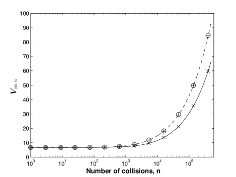
Figure 1: Numerical results for ${V}_{rms}$ of an ensemble of $10^{4}$ particles evolving in a FUM with two oscillating walls as a function of the number of collisions. Results were obtained by iterating the exact (circles) as well as the corresponding static (diagonal crosses) and hopping wall (upright crosses) approximative maps. It is noted that $V_{rms}$ is measured in units of $\omega w$. Analytical results according to the SWA averaged over the random phase (solid line) as well as the analytical prediction according to eq.(7) (dash-dotted line) are also shown.

The above analysis reveals the role of the fluctuations in the time of flight $\delta{t}_{n}$ between successive collisions caused by the displacement of the scatterer. Despite the existence of an external stochastic component in the phase of the oscillating wall these fluctuations lead to a systematic increase of the acceleration of the particles. A simple explanation of the physical mechanism leading to the increased acceleration becomes possible by considering the various configurations of the collision processes between the wall and the particles. Let us assume for a given velocity of the incident particle that the wall is moving in the same direction as the particle after passing the equilibrium position. The collision time due to wall displacement increases then, compared to the one assuming a wall fixed in space. In this case, the velocity of the harmonically oscillating wall is a decreasing function of time and therefore an increase of the collision time leads to a decrease of the wall velocity on the actual instant of the collision when compared to the static wall approximation. This in turn leads to a lesser energy loss in the course of the collision. This reasoning holds equally in all other types of collision events, leading to the general picture of less energy loss or more energy gain when the wall displacement is taken into account.

The focus of our attention now shifts to the probability distribution function (PDF) of the magnitude of the particle velocity and number of collisions $n$, $\rho(|V|,n)$. It has been shown that the change of $\langle{V}^{2}\rangle$ as a function of the number of collisions $n$ can be accurately described by a random walk in momentum space $\langle V^{2}\rangle\propto n$, provided that the spatial motion of the walls is taken into account. Numerical as well as analytical treatments in setups similar to the present one suggest that $\rho(|{V}|,n)$ is described by a spreading Gaussian Bouchet:2004 ; Ott:1993 . However, simulations with the exact map of eq.(1) yield the histograms in Figs. 2a,b $\rho(|V|,n)$ which show the PDFs corresponding to snapshots for $n=5\cdot 10^{4}$, $5\cdot 10^{5}$ collisions. It is shown that, even if the initial PDF is a Gaussian, with increasing time, it is transformed to a one-dimensional Maxwell-Boltzmann-like distribution since the set of initial conditions leading to $|{V}|\ll 1$ is vanishingly small for sufficiently long times. Using the hopping wall map the following analytical expression for the PDF is obtained, which describes the magnitude of the particle velocity for $n\gg 1$:

$$\rho(|{V}|,n)=\frac{1}{\sigma^{2}}|{V}|e^{-\frac{{V}^{2}}{2\sigma^{2}}}$$ (8)

where $\sigma=\sqrt{\frac{4\epsilon^{2}n+\langle{V}_{0}^{2}\rangle}{2}}$. In Figs. 2a,b it is clearly seen that this analytical result predicted by the HWA accurately reproduces the exact behavior of the system. Furthermore, Fig. 2(c) shows the evolution of the mean value $\langle|V|\rangle$ as a function of the number of collisions $n$ obtained numerically using the exact dynamics (open circles). For the sake of comparison we also show the corresponding analytical result: $\langle|V|\rangle=\sqrt{\frac{\pi}{2}}\sigma$ based on eq.(8) (solid line).

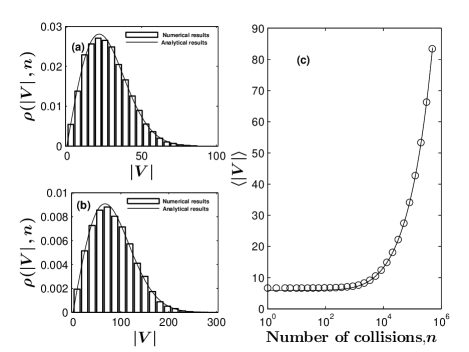
Figure 2: Numerically computed PDF for the magnitude of particle velocity using an ensemble of $10^{4}$ trajectories and following the exact dynamics of eq.(1) for: (a) $n=5\cdot 10^{4}$ and (b) $n=5\cdot 10^{5}$. In each case the analytical result given by eq.(8) using the HWA is also shown (solid line). Finally, (c) shows the numerically obtained evolution of $\langle|{V}|\rangle$ as a function of $n$ using the exact dynamics (open circles) as well as the analytical approximation based on eq.(8) (solid line).

The development of hyper-acceleration takes place in higher-dimensional scattering systems as well, such as a time-dependent Lorentz gas consisting of harmonically oscillating circular hard scatterers on a triangular lattice. It is emphasized that in the time-dependent Lorentz gas system Fermi acceleration exists without any externally imposed randomization Loskutov ; Leonel:2005 . However, the absence or presence of a random component in the dynamics influences the acceleration law. For example, if the oscillation axis is fixed and uniform throughout the lattice the acceleration law is $V_{rms}\propto n^{1/4}$. On the other hand, if the oscillation axis of the disks is randomly chosen on each collision, simulating the effect of thermal noise, the acceleration law becomes $V_{rms}\propto n^{1/2}$, as in the 1D FUM system Karlis:2006 . In both cases, the static approximation underestimates the ensemble mean energy growth while the hopping approximation provides results much closer to those of the exact model. To illustrate this, in Fig. 3 numerical results for the random setup outlined above are presented. These are obtained utilizing the exact map Papachristou:2001 , as well as the corresponding hopping and static approximative maps . Consequently, it can be inferred that the development of hyper-acceleration is common to many driven dynamical systems, and features in any billiard which allows Fermi acceleration to develop. Moreover, the understanding gained in the present investigation helps open up the prospect of designing time-laws for the driving that provide a specified acceleration behavior for the ensemble of particles thus leading to a desired non-equilibrium i.e. time-evolving velocity distribution.

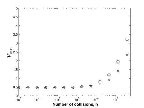
Figure 3: Numerical results for ${V}_{rms}$ of an ensemble of $10^{4}$ particles evolving in a triangular harmonically driven Lorentz gas with randomly chosen direction of oscillation on each collision, as a function of the number of collisions. Results were derived by iterating the exact maps (circles) as well as the corresponding static (diagonal crosses) and hopping (upright crosses) approximations. The parameters $\left|{\rm{\bf A}}\right|=0.01$, $\omega=1$, $w=2.15$, $V_{0}=\frac{1}{2.15}$ have been used in the numerical simulations, with $A$ denoting the magnitude of the amplitude of oscillation, $\omega$ the angular frequency, $w$ the spacing between the disk centers at equilibrium and $V_{0}$ the initial particle velocity. Velocities are measured in units $\omega w$.

References

- (1) E. Fermi, Phys. Rev. 75, 1169 (1949).
- (2) R. Blandford, D. Eichler, Phys. Rep. 154, 1 (1987).
- (3) A. Veltri and V. Carbone, Phys. Rev. Lett. 92 143901 (2004).
- (4) K. Kobayakawa, Y.S. Honda and T. Samura, Phys. Rev. D 66 083004 (2002).
- (5) M. A. Malkov, Phys. Rev. E 58, 4911 (1998).
- (6) G. Michalek, M. Ostrowski and R. Schlickeiser, Sol. Phys. 184, 339 (1999).
- (7) A. V. Milovanov and L. M. Zelenyi, Phys. Rev. E 64, 052101 (2001).
- (8) F. Saif, I. Bialynicki-Birula, M. Fortunato, W. P. Schleich, Phys. Rev. A 58, 4779 (1998).
- (9) A. Steane, P. Szriftgiser, P. Desbiolles, J.Dalibard, Phys. Rev. Lett. 74, 4972 (1995).
- (10) G. Lanzano et al, Phys. Rev. Lett. 83, 4518 (1999).
- (11) A. Yu. Loskutov, A. B. Ryabov, and L. G. Akinshin, J. Exp. Theor. Phys. 89, 966 (1999); J. Phys. A: Math. Gen. 33 7973 (2000).
- (12) S. Ulam, in Proceedings of the Fourth Berkley Symposium on Mathematics, Statistics, and Probability, California U.P., Berkeley, 1961, Vol. 3, p. 315.
- (13) M. A. Lieberman and A. J. Lichtenberg, Phys. Rev. A 5, 1852 (1972).
- (14) A. J. Lichtenberg, M. A. Lieberman, Regular and Chaotic Dynamics, Applied Mathematical Sciences, 38, Springer Verlag, New York, 1992.
- (15) Z. J. Kowalik, M. Franaszek and P. Pieranski, Phys. Rev. A 37, 4016 (1988).
- (16) S. Warr et al, Physica A 231, 551 (1996).
- (17) S. Celaschi and R. L. Zimmerman, Phys. Lett. A 120, 447 (1987).
- (18) E. D. Leonel, J. K. L. da Silva and S. O. Kamphorst, Physica A 331, 435 (2004).
- (19) E. D. Leonel and P. V. E. McClintock, J. Phys. A 38, 823 (2005).
- (20) A. J. Lichtenberg, M. A. Lieberman and R. H. Cohen, Physica D 1, 291 (1980).
- (21) E. D. Leonel, P. V. E. McClintock and J. K. da Silva, Phys. Rev. Lett. 93, 014101 (2004).
- (22) A. Einstein, Investigations on the Theory of the Brownian Movement, Dover, New York, 1956.
- (23) G. M. Zaslavskii and B. V. Chirikov, Sov. Phys. Doklady 9, 989 (1965).
- (24) A. Brahic, Astron. and Astrophys. 12, 98 (1971).
- (25) A. K. Karlis et al, in preparation.
- (26) F. Bouchet, F. Cecconi and A. Vulpiani, Phys. Rev. Lett. 92, 040601 (2004).
- (27) E. Ott, Chaos in Dynamical Systems, Cambridge University Press, Cambridge, 1993.
- (28) P. K. Papachristou, F. K. Diakonos, E. Mavrommatis, and V. Constantoudis, Phys. Rev. E 64, 016205 (2001).