High-Order-Mode Soliton Structures in Two-Dimensional Lattices with Defocusing Nonlinearity

Abstract

While fundamental-mode discrete solitons have been demonstrated with both self-focusing and defocusing nonlinearity, high-order-mode localized states in waveguide lattices have been studied thus far only for the self-focusing case. In this paper, the existence and stability regimes of dipole, quadrupole and vortex soliton structures in two-dimensional lattices induced with a defocusing nonlinearity are examined by the theoretical and numerical analysis of a generic envelope nonlinear lattice model. In particular, we find that the stability of such high-order-mode solitons is quite different from that with self-focusing nonlinearity. As a simple example, a dipole (“twisted”) mode soliton which may be stable in the focusing case becomes unstable in the defocusing regime. Our results may be relevant to other two-dimensional defocusing periodic nonlinear systems such as Bose-Einstein condensates with a positive scattering length trapped in optical lattices.

I Introduction

Ever since the suggestion of optically induced lattices in photorefractive media such as Strontium Barium Niobate (SBN) in efrem , and its experimental realization in moti1 ; neshevol03 ; martinprl04 , there has been an explosive growth in the area of nonlinear waves and solitons in periodic lattices. A stunning array of structures has been predicted and experimentally obtained in lattices induced with a self-focusing nonlinearity, including (but not limited to) discrete dipole dip , quadrupole quad , necklace neck and other multi-pulse patterns (such as e.g. soliton stripes multi ), discrete vortices vortex , and rotary solitons rings . Such structures have a potential to be used as carriers and conduits for data transmission and processing, in the context of all-optical schemes. A recent review of this direction can be found in moti3 (see also zc4 ).

Many of these studies in induced lattices were also triggered by the pioneering work done in fabricated AlGaAs waveguide arrays 7 . In the latter setting a multiplicity of phenomena such as discrete diffraction, Peierls barriers, diffraction management 7a and gap solitons 7b among others eis3 were experimentally obtained. These phenomena, in turn, triggered a tremendous increase also on the theoretical side of the number of studies addressing such effectively discrete media; see e.g. review_opt ; general_review for a number of relevant reviews.

Finally, yet another area where such considerations and structures are relevant is that of soft-condensed matter physics, where droplets of Bose-Einstein condensates (BECs) may be trapped in an (egg-carton) two-dimensional optical lattice potential bloch . The latter field has also experienced a huge growth over the past few years, including the prediction and manifestation of modulational instabilities pgk , the observation of gap solitons markus and Landau-Zener tunneling arimondo among many other salient features; reviews of the theoretical and experimental findings in this area have also been recently appeared in konotop ; markus2 .

In light of all the above activity, it is interesting to note that the only structure that has been experimentally observed in two-dimensional (2d) lattices in “defocusing” media consists of self-trapped “bright” wave packets (so-called “staggered” or gap solitons) excited in the vicinity of the edge of the first Brillouin zone moti1 . However more complex coherent structures have not yet been explored in lattices with defocusing nonlinearity and their stability properties have not yet been examined, to the best of our knowledge. It should be mentioned that the defocusing context is accessible in the aforementioned settings. E.g., in the photorefractive lattices, this can be done by appropriate reversal of the applied voltage to the relevant crystal, while in BECs, the defocusing nonlinearity corresponds to the most typical case arising in dilute gases of ⁸⁷Rb or ²³Na.

It is the aim of the present work to examine the non-fundamental soliton structures (e.g., dipoles, multipoles, and vortices) in lattices with a defocusing nonlinearity, and to illustrate the similarities and differences in comparison to their counterparts in the focusing case. In particular, we study dipole structures (consisting of two peaks) and quadrupole structures (featuring four peaks), as well as vortices of topological charge $S=1$ (cf. vortex ) in a 2D induced lattice with a defocusing nonlinearity. These structures will be analyzed in detail for both cases, namely, the “on-site” excitation (where the center of the structure is on an empty lattice site between the excited ones) and the “inter-site” excitation (where their center is between two lattice sites and no empty lattice site exists between the excited ones).

Our study of these structures will be conducted analytically and numerically (in the next two sections) in the context of the most prototypical generic envelope lattice model, the so-called discrete nonlinear Schrödinger (DNLS) equation with a defocusing nonlinearity dnls which is related to all of the above contexts review_opt ; konotop . When we find the relevant structures to be unstable, we will also briefly address the dynamical evolution of the instability, through appropriately crafted numerical experiments. Finally, in the last section, we will summarize our findings and present our conclusions, and the interesting experimental manifestations that they suggest.

II Model and Theoretical Setup

As our generic envelope model encompassing the main features of discrete diffraction and defocusing nonlinearity we use the two-dimensional (2D) DNLS equation:

$$i\dot{u}_{\mathbf{n}}=-C\left(\Delta_{2}u\right)_{\mathbf{n}}+|u_{\mathbf{n}}|^{2}u_{\mathbf{n}},$$ (1)

where $u_{\mathbf{n}}$ is a complex amplitude of the electromagnetic wave in nonlinear optics review_opt , or the BEC wave function at the nodes of a deep 2D optical lattice konotop ; $\mathbf{n}$ is the (two-dimensional in the present study) vector lattice index, and $\Delta_{2}$ the standard discrete Laplacian. Furthermore, $C$ is the constant of the intersite coupling (associated with the interwell “tunnelling rate” konotop ), and the overdot stands for the derivative with respect to the evolution variable, which can be $z$ in optical waveguide arrays, or the time $t$ in the BEC model. We focus on standing-wave solutions of the form $u_{\mathbf{n}}=\exp(-i\Lambda t)\phi_{\mathbf{n}}$, with $\phi_{\mathbf{n}}$ satisfying the equation,

$$f(\phi_{\mathbf{n}},C)\equiv-\Lambda\phi_{\mathbf{n}}-C\Delta_{2}\phi_{\mathbf{n}}+|\phi_{\mathbf{n}}|^{2}\phi_{\mathbf{n}}=0.$$ (2)

Perturbing around the solutions of Eq. (2) gives rise to the linearization operator

$$\mathcal{H}_{\mathbf{n}}^{(C)}=\left(\begin{array}[]{cc}-\Lambda+2|\phi_{\mathbf{n}}|^{2}&\phi_{\mathbf{n}}^{2}\\ \bar{\phi}_{\mathbf{n}}^{2}&-\Lambda+2|\phi_{\mathbf{n}}|^{2}\end{array}\right)-C\Delta_{2}\left(\begin{array}[]{cc}1&0\\ 0&1\end{array}\right),$$ (7)

with the overbar denoting complex conjugation. Through an appropriate rescaling of the equation, we can fix $\Lambda\equiv 1$. Our analysis uses as a starting point the so-called anti-continuum limit, i.e., the case of $C=0$, where for the uncoupled sites,

$$\phi_{\mathbf{n}}=r_{\mathbf{n}}e^{i\theta_{\mathbf{n}}},$$ (8)

with the amplitude $r_{\mathbf{n}}$ being $0$ or $\sqrt{\Lambda}$, and the phase $\theta_{\mathbf{n}}$ being an arbitrary constant. Continuation of such a solution to nontrivial couplings necessitates that a certain, so-called Lyapunov-Schmidt condition be satisfied dep . The latter imposes for the projection of eigenvectors of the kernel of $\mathcal{H}_{\mathbf{n}}^{(0)}$ onto the system of stationary equations to be vanishing. This solvability condition provides a nontrivial constraint at every “excited” (i.e., $r_{\mathbf{n}}\neq 0$) site of the AC limit, namely:

$$-2ig_{\mathbf{n}}(\theta,C)\equiv-Ce^{-i\theta_{\mathbf{n}}}\Delta_{2}\phi_{\mathbf{n}}+Ce^{i\theta_{\mathbf{n}}}\Delta_{2}\bar{\phi}_{\mathbf{n}}=0.$$ (9)

It is interesting (and crucial for stability purposes) to note that this equation has an extra $(-)$ sign in comparison to its focusing counterpart. The derivation of these solvability conditions is especially important because the corresponding Jacobian

$$\mathcal{M}_{ij}=\partial g_{i}/\partial\theta_{j}$$ (10)

has eigenvalues $\gamma$ that are directly related to the “regular” eigenvalues of the linearization problem $\lambda$, through the equation

$$\lambda=\pm\sqrt{2\gamma}.$$ (11)

Hence, the method that we use to derive the eigenvalues $\lambda$ (which fully determine the crucial issue of stability of the solution for small $C$) consists of a perturbative expansion of the solution from the AC limit

$$\phi_{\mathbf{n}}=\phi_{\mathbf{n}}^{(0)}+C\phi_{\mathbf{n}}^{(1)}+\dots,$$ (12)

which allows us to derive the principal bifurcation conditions for a specific configuration and therefore infer its linear stability properties through the eigenvalues of $\mathcal{M}$ and their connection to the linearization eigenvalues $\lambda$. Recall that a nonzero real part of any eigenvalue is a necessary and sufficient condition for an exponential instability in Hamiltonian systems, such as the one considered herein.

III Comparison of Analytical and Numerical Results

III.1 General Terminology

We start with some general terminology that we will use in this section. The designation in-phase (IP) will be used for two sites such that their relative phase difference is $0$, while out-of-phase (OP) will signify that it is $\pi$. Furthermore, on-site (OS) will mean that the center of the configuration is on an empty lattice site (between the excited ones), while inter-site (IS) will signify that the center is located between the excited lattice sites (and no empty site exists between them). For all modes, in the figures below, we show their power $P=\sum|u_{\mathbf{n}}|^{2}$ as a function of the coupling strength $C$, as well as the real and imaginary parts of the key eigenvalues (the ones determining the stability of the configuration). We start with the dipole configuration (consisting primarily of two lattice sites; see Figs. 1-4). We also examine the more complex quadrupole (see Figs. 5-8) and vortex (see Figs. 9-10) configurations. In all the cases, we offer typical examples of the mode profiles and stability for select values of $C$. When the configurations are found to be unstable, we also give a typical example of the instability evolution, for a relevant value of the coupling strength. Another general feature that applies to all modes is a continuous spectrum band extending for $\lambda_{i}\in[\Lambda-8C,\Lambda]$. This latter trait significantly affects the stability intervals of the structures in comparison with their focusing counterparts as we will see also below (since configurations may be stable for small $C$, but not for larger $C$).

The presentation of the figures will be uniform throughout the manuscript in that in each pair of figures, we examine two types of configurations (one in the left column and one in the right column). The first figure of each pair will have five panels showing $P$ as a function of $C$, the principal real eigenvalues (second panel) and imaginary eigenvalues (third panel). In these plots, the numerical results are shown by the solid (blue) line, while the analytical results by the dashed (red) line. The fourth and fifth panels show typical examples of the relevant configuration (obtained through a fixed point iteration of the Newton type) and its stability eigenvalues (shown through the spectral plane $(\lambda_{r},\lambda_{i})$ for the eigenvalues $\lambda=\lambda_{r}+i\lambda_{i}$). The accompanying second figure will show the result of a typical evolution of an unstable mode, perturbed by a random perturbation of amplitude $10^{-4}$, in order to accelerate the instability evolution. The four contour plot panels (one set on the left and one on the right) will display the solution’s squared absolute value for four different values of the evolution variable; the bottom panel will show the dynamical evolution of the sites chiefly “participating” in the solution. A fourth-order Runge-Kutta scheme has been used for the numerical integration results presented herein.

To facilitate the reader, a summary of the results, encompassing our main findings reported below is offered in Table 1. The table summarizes the configurations considered, their linear stability and the outcome of their dynamical evolution for appropriate initial conditions in the instability regime. Note that if the solutions are unstable for all $C$, they are denoted as such, while if they are partially stable for a range of coupling strengths, their interval of stability is explicitly mentioned. Details of our analytical results and their connection/comparison with the numerical findings are offered in the rest of this section.

	On-site		Inter-site
Type	Stability	Instability Outcome	Stability	Instability Outcome
In-phase Dipole	Unstable	1-Site Pulse	$C<0.064$	1-Site Pulse
Out-of-phase Dipole	$C<0.092$	Decay	Unstable	1-Site Pulse
In-phase Quadrupole	Unstable	Breathing Behavior	$C<0.047$	1-Site Pulse
Out-of-phase Quadrupole	$C<0.08$	1-Site Pulse	Unstable	2-Site Mode
Vortex	$C<0.095$	1-Site Pulse	$C<0.095$	1-Site Pulse

Table 1: Summary of the stability results for all the configurations presented below. For partially stable (near the anti-continuum limit) solutions their interval of stability (for $\Lambda=1$) is given. In each case, the outcome of the instability evolution for the parameters and initial conditions considered below is also mentioned.

III.2 Dipole Configurations

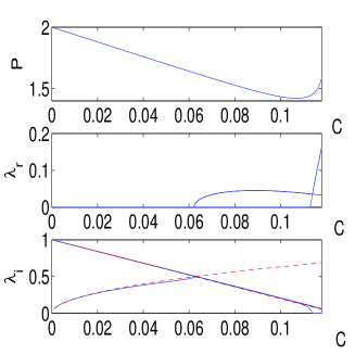
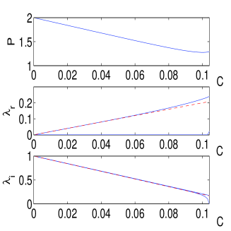
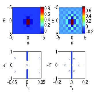
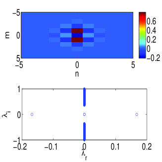
Figure 1: (Color Online) The first line of panels shows the power $P$ vs. coupling $C$ for the inter-site (IS), in-phase (IP) mode (left) and on-site (OS), IP mode (right). The second lines show their maximal real eigenvalues and the third their first few imaginary eigenvalues. The solid (blue) lines illustrate the numerical results, while the dashed (red) lines the analytical ones. The fourth and fifth panels show the contour plot of the mode profile (fourth panel) and the corresponding spectral plane of eigenvalues $\lambda=\lambda_{r}+i\lambda_{i}$ (fifth panel); The left two panels are for the IS-IP mode for $C=0.08$ and $C=0.116$ respectively. The right panel shows the OS-IP mode for $C=0.08$.

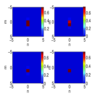
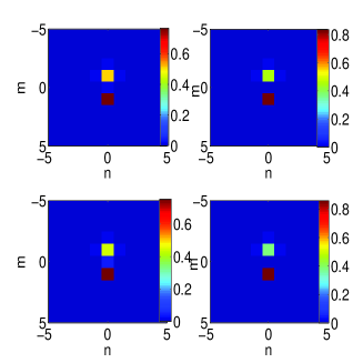
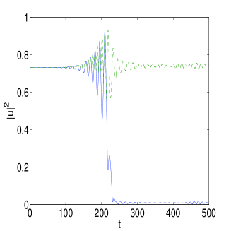
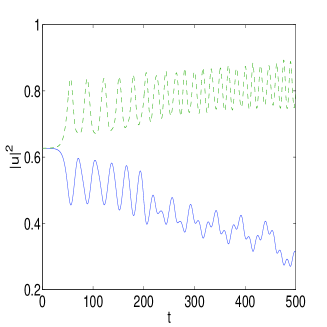
Figure 2: (Color Online) The four panels at the top left corner show the contour plots of the dynamical evolution of the unstable inter-site, in phase (IS-IP) solution for $C=0.08$. The respective times are $t=50$ and $t=150$ in the top and $t=250$ and $t=350$ in the second row. The panel at the bottom left shows the dynamical evolution of the square modulus of the principal two sites participating in the IS-IP solution as a function of time. From both of the above, it is clear that the configuration relaxes into a single site soliton. The right panels show the same features for the on-site, in-phase (OS-IP) solution, which also relaxes (but more slowly) into a single-site configuration.

III.2.1 Inter-site, In-Phase Mode

Figures 1-2 encompass our results for the two types of IP dipole solutions (i.e., initialized at the AC limit with two in-phase excited sites). The IS-IP mode of the left panels is theoretically found to possess 1 imaginary eigenvalue pair (and, hence, is stable for small $C$)

$$\lambda\approx\pm 2\sqrt{C}i.$$ (13)

The collision with the continuous spectrum described above causes the mode to become unstable for sufficiently large $C$; the theoretically predicted instability threshold (obtained by equating the eigenvalue of Eq. (13) with the lower edge of the phonon band located at $\Lambda-8C$) is $C=0.0625$, the numerically found one is $C\approx 0.064$. Additional instability may ensue when the monotonicity of the $P$ vs. $C$ curve changes (we have found this to be a general feature of the defocusing branches). The fourth and fifth panels show the mode and its linearization eigenvalues for $C=0.08$ and $C=0.116$. In fact, the dynamical evolution of the mode is demonstrated for the case of $C=0.08$, illustrating that only one of the two sites eventually persists, after the demonstrably oscillatory instability destroys the configuration for $t>100$.

III.2.2 On-site, In-Phase Mode

The OS-IP mode of the right panels of Figs. 1-2 is always unstable due to a real pair, theoretically found to be

$$\lambda\approx\pm 2C,$$ (14)

for small $C$. Notice once again the remarkable accuracy of this theoretical prediction, in comparison with the numerically obtained eigenvalue. The fourth and fifth right panels of Fig. 1 show the mode and its stability for $C=0.08$. Its dynamical evolution in the right column of Fig. 2 shows its slow disintegration into a single-site solitary wave.

III.2.3 Inter-site, Out-of-phase Mode

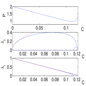
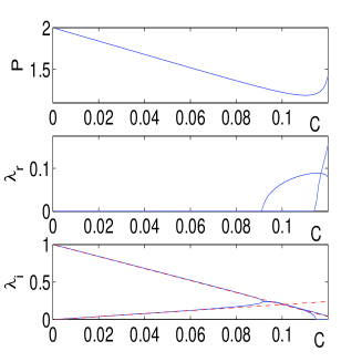
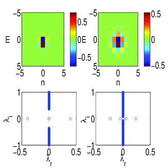
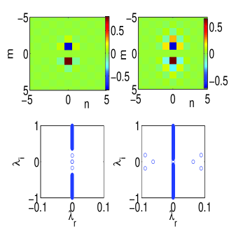
Figure 3: (Color Online) Similar to Fig. 1, but now for the inter-site, out-of-phase (IS-OP) mode (left panels) and for the on-site, out-of-phase mode (OS-OP). The fourth and fifth rows of panels are for $C=0.08$ and for $C=0.116$ in both cases.

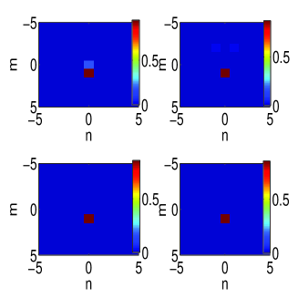
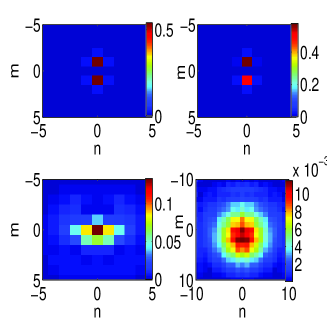
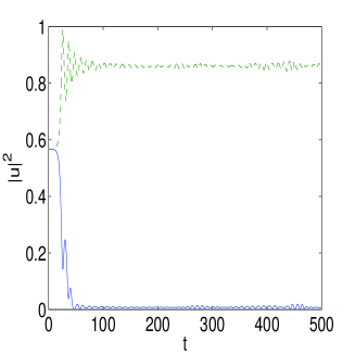
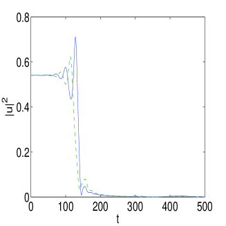
Figure 4: (Color Online) Same as in Fig. 2, but now for the IS-OP mode (left panels) and the OS-OP mode (right panels). The former shown at times $t=25$, $t=50$ (top row), $t=150$ and $t=250$ (second row), in the case of $C=0.08$ finally results into a single-site configuration (as is also illustrated by the bottom panel showing the two principal sites participating in the mode). The latter, shown for $C=0.1$, at times $t=50$, $t=100$ (top row), $t=150$ and $t=200$ (second row) is entirely destroyed by the instability resulting into small amplitude excitations.

Figures 3-4 illustrate the two dipole, out-of-phase modes. The left panels of the figures correspond to the IS-OP mode; this one is also immediately unstable (as one departs from the anti-continuum limit), due to a real pair which is

$$\lambda\approx 2\sqrt{C},$$ (15)

for small $C$. The fourth and fifth panels of Fig. 3 show the relevant mode for $C=0.08$ and $C=0.116$, showing its 1 and 2 unstable real eigenvalue pairs respectively. The numerical experiment highlighting the evolution of the mode for the case of $C=0.08$ is shown in the left panel of Fig. 4. Clearly, in this case as well, the positive real eigenvalue leads to the growth of one of the two sites constituting the dipole, and the eventual formation of a single-site solitary pulse.

III.2.4 On-site, Out-of-phase Mode

The right panels of Fig. 3-4 show the OS-OP mode. The stability analysis of this waveform shows that it possesses an imaginary eigenvalue

$$\lambda\approx 2Ci.$$ (16)

This leads to an instability upon collision (occurring theoretically for $C=0.1$, numerically for $C\approx 0.092$) with the lower edge (located at $\Lambda-8C$) of the continuous band of phonon modes. The mode is shown for $C=0.08$ and $C=0.116$ in the right panels of Fig. 3. The direct integration of the unstable solution with $C=0.1$ is shown in the right panels of Fig. 4, indicating that in this case the mode completely disappears (because of the oscillatory instability) into extended wave, small amplitude radiation.

III.3 Quadrupole Confirgurations

III.3.1 Inter-site, In-phase Mode

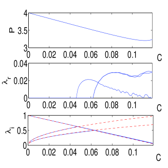
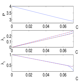
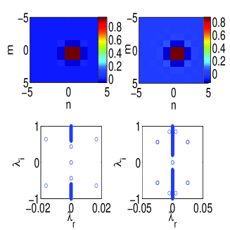
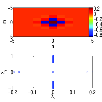
Figure 5: (Color Online) The top three lines of panels show the same features as the corresponding ones of figure 1 but now for the quadrupole IS-IP mode (left) and the quadrupole OS-IP mode (right). The contour plot of the real part of the modes and the spectral plane of their linearization eigenvalues are shown in the fourth and fifth rows for $C=0.05$ and $C=0.1$ in the case of the former mode, while the latter is only shown for $C=0.05$.

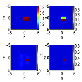
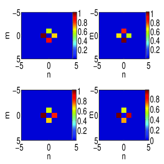
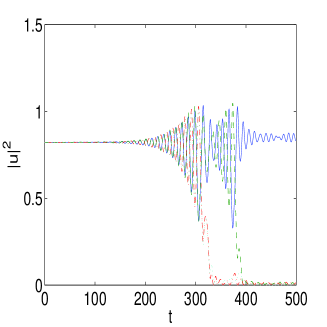
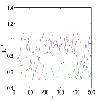
Figure 6: (Color Online) Same as Fig. 2, but now for the quadrupole IS-IP mode with $C=0.08$ (left panels) and the quadrupole OS-IP mode with $C=0.05$ (right panels). The left panels are for $t=200$, $t=300$ (top), $t=400$ and $t=500$ (middle) and illustrate alongside the bottom panel (containing the evolution of the principal four sites participating in the structure) how the configuration eventually degenerates to a single-site soliton. The right panels are for $t=50$, $t=150$, (top row) $t=250$ and $t=350$ (second row) and show together with the bottom panel the complex oscillation (breathing) involved in the behavior of the quadrupole OS-IP mode for $C=0.05$.

Figures 5-6 show the quadrupolar mode with four in-phase participating sites when centered between lattice sites in the left panels of the figures. This mode is theoretically predicted to have two imaginary (for small $C$) eigenvalue pairs with

$$\lambda\approx 2\sqrt{C}i$$ (17)

and one imaginary pair with

$$\lambda\approx\sqrt{8C}i.$$ (18)

As a result, this mode (shown in the fourth row panels of Fig. 5 for $C=0.05$ and $C=0.1$) is unstable due to the collision of the above eigenvalues with the continuous spectrum occurring theoretically for $C\approx 0.0477$, while in the numerical computations it happens for $C\approx 0.047$. The outcome of the instability shown in Fig. 6 for $C=0.08$ is the degeneration of the quadrupolar mode into a single-site excitation.

III.3.2 On-site, In-phase Mode

The right panels of Figs. 5-6 show the case of the on-site, in-phase mode. The latter is found to always be unstable due to a real eigenvalue pair of

$$\lambda\approx\pm 4C$$ (19)

and a double, real eigenvalue pair of

$$\lambda\pm\sqrt{12}C.$$ (20)

This can also be clearly observed in the fourth and fifth panels of Fig. 5, showing the mode and its stability for $C=0.05$. The dynamical evolution of the unstable mode for $C=0.05$ is shown in the panels of Fig. 6. Both from the contour plots at the different times and from the dynamical evolution of the main sites participating in the structure, it can be inferred that the mode embarks in an oscillatory breathing, without being ultimately destroyed in this case.

III.3.3 Inter-site, Out-of-Phase Mode

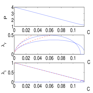
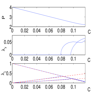
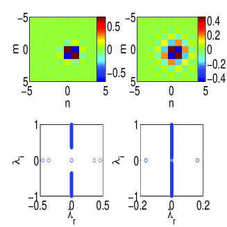
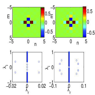
Figure 7: (Color Online) Similar to Fig. 1 but for the quadrupole IS-OP mode (left panels) and the quadrupole OS-OP mode (right panels). The fourth and fifth rows show the modes and their stability for $C=0.08$ and $C=0.116$ in each case.

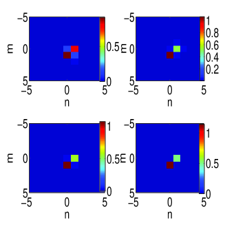
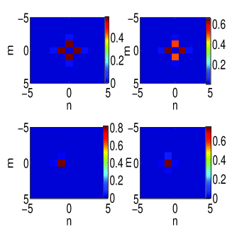
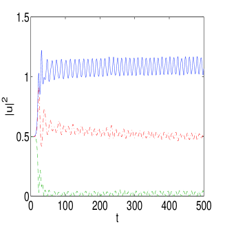
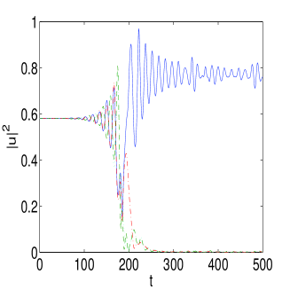
Figure 8: (Color Online) Same as Fig. 2, but for the evolution of the quadrupole IS-OP mode with $C=0.08$ (left panels) the quadrupole OS-OP mode with $C=0.1$ (right panels). The former is shown for $t=25$, $t=50$ (top row), $t=150$ and $t=250$ (second row) substantiating (together with the bottom panel showing the principal four sites of the branch) its resulting into a long-lived, breathing two-site waveform. The latter is shown for $t=50$, $t=150$ (top row), $t=250$ and $t=350$ (second row) indicating its degeneration into a single-site configuration.

We next consider the case of the IS-OP mode in Figs. 7-8. Our analytical results for this mode show that for small values of $C$, we should expect to find it to be immediately unstable due to three real pairs of eigenvalues, namely a single one with

$$\lambda\approx\pm\sqrt{8C}$$ (21)

and a double one with

$$\lambda\approx\pm 2\sqrt{C}.$$ (22)

This expectation is once again confirmed by the numerical results of the left panel of Fig. 7. The fourth and fifth panels show the mode and the spectral plane of its linearization for the cases of $C=0.08$ and $C=0.116$. The dynamical evolution of this mode also gives an interesting result, in that it produces, upon manifestation of the instability, a long-lived, two-site oscillatory mode, as is illustrated in the left panels of Fig. 8 for $C=0.08$.

III.3.4 On-site, Out-of-phase Mode

Finally, the last one among the quadrupolar modes is the OS-OP mode, examined in the right panels of Figs. 7-8. Our theoretical analysis predicts that this mode should have a double imaginary eigenvalue pair of

$$\lambda\approx\pm 2Ci$$ (23)

and a single imaginary pair of

$$\lambda\approx 4Ci.$$ (24)

These, in turn, imply that the mode is stable for small $C$, but becomes destabilized upon collision of the larger one among these eigenvalues with the continuous band of phonons. This is numerically found to occur for $C\approx 0.08$, while it is theoretically predicted, based on the above eigenvalue estimates, to take place for $C=0.083$. The mode’s stability analysis is shown in the fourth and fifth panel of Fig. 7 for $C=0.08$ and $C=0.116$; for $C=0.1$, and its dynamical evolution is examined in the right panels of Fig. 8. In this case, we do find that the mode essentially degenerates to a single-site solitary wave.

III.4 Vortex Configuration

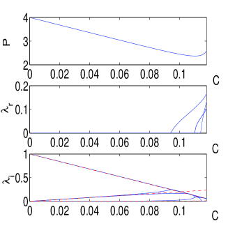
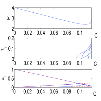
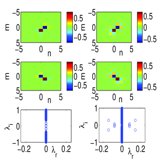
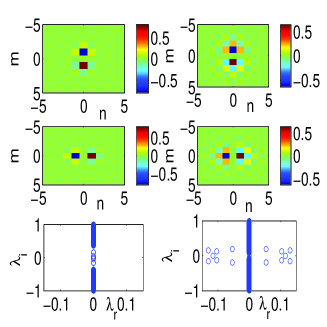
Figure 9: (Color Online) The same features as in Figure 1 are shown here for the IS vortex of topological charge $S=1$ (left) and the OS vortex of $S=1$ (right). In this case both the real (fourth line) and imaginary (fifth line) parts of the solution are shown (and their stability in the sixth line) for $C=0.08$ and $C=0.116$.

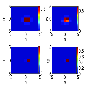
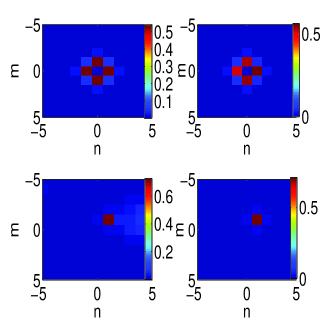
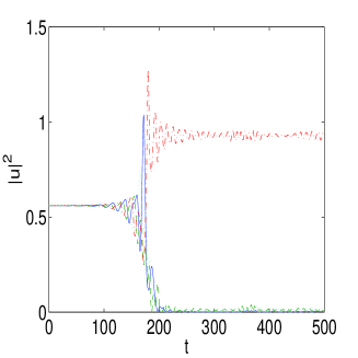
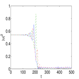
Figure 10: (Color Online) Same as in Fig. 2 but for the dynamical evolution of the IS (left panels) and the OS (right panels) vortex of topological charge $S=1$. Both cases are shown for $C=0.1$. Both the left and right panels of evolution are for $t=50$, $t=150$ (top row), $t=250$ and $t=350$ (second row) and alongside the bottom panels showing the principal four sites of the vortex they show how the vortices transform themselves into fundamental solitary waves centered on a single site (in the latter case, interestingly, the site of the largest excitation of the ensuing wave is not one among the four principal excitation sites of the original OS vortex).

III.4.1 Inter-site Vortices

Finally, Figs. 9-10 show similar features, but now for the IS (left panels) and OS (right panels) vortex solutions dnls ; dep . The former has a theoretically predicted double pair of eigenvalues

$$\lambda\approx\pm 2Ci.$$ (25)

leading to an instability upon collision with the continuum band for $C\geq 0.095$ ($C\geq 0.1$ theoretically). In this case, there is also an eigenvalue of higher order

$$\lambda\approx\pm 4C^{2}i.$$ (26)

which obviously depends more weakly on $C$. The fourth and fifth panels of Fig. 9 show the real and the imaginary parts of the vortex configuration for $C=0.08$ and $C=0.116$ and the sixth panel the corresponding spectral planes. The dynamical evolution of the vortex of topological charge $S=1$, for $C=0.1$ is shown in the left panels of Fig. 10, indicating that the vortex also, upon the occurrence of the oscillatory instability, becomes a single-site solitary wave.

III.4.2 On-site Vortices

On the other hand, the OS vortices are shown in the right panels of Figs. 9-10. In this case, we theoretically find that the vortex, for small $C$, should have a double pair of eigenvalues

$$\lambda\approx 2Ci$$ (27)

and a single, higher order pair of eigenvalues

$$\lambda\approx\pm\sqrt{32}C^{3}i.$$ (28)

The former eigenvalue pairs, upon collision with the continuous spectrum, lead to an instability, theoretically predicted to occur at $C=0.1$ and numerically found to happen for $C\approx 0.095$. The on-site mode (and its stability) is shown in the fourth-sixth right panels of Fig. 9 for $C=0.08$ and $C=0.116$. Its evolution (for $C=0.1$) is shown in the right panel of Fig. 10, where it is again seen that the mode degenerates from an $S=1$ to an $S=0$ structure, i.e., a single-site solitary wave with no topological charge.

III.5 General Principles Derived From Stability Considerations

It is interesting to note as an over-arching conclusion that the stability intervals of the defocusing structures are different from those of their focusing counterparts (especially when they are stable close to the AC limit) because of the collisions with the continuous spectrum band edge; the latter is at $\lambda=\Lambda$ in the focusing case, while it is at $\lambda=\Lambda-8C$ in the defocusing setting. Another similarly general note is an immediate inference on whether the structures are stable or not; this can be made based on the knowledge of whether their focusing counterparts are stable or not and the transformation from the former to the latter through the staggering transform: $u_{n,m}=(-1)^{n+m}v_{n,m}$. For instance, IP two-site configurations (both OS and IS) are known to be generically unstable in the focusing regime dep ; through the staggering transformation, OS-IP of the focusing case remains OS-IP in the defocusing, while IS-IP of the focusing becomes IS-OP in the defocusing. Hence, these two should be expected to be always unstable, while the remaining two (OS-OP in both focusing and defocusing and IS-OP of the focusing, which becomes IS-IP in the defocusing) should similarly be expected to be linearly stable close to the AC-limit, as is indeed observed. Notice that, interestingly enough, for the vortex states the staggering transformation indicates that the stability is not modified between the focusing and defocusing cases. This is because for an IS vortex, it transforms an $S=1$ state into an $S=-1$ state (which is equivalent to the former, in terms of stability properties), while the OS vortex remains unchanged by the transformation. However, as mentioned above, these considerations are not sufficient to compute the instability thresholds for initially stable modes, among other things. They do, nonetheless, provide a guiding principle for inferring the near-AC limit stability of the defocusing staggered states, based on their focusing counterparts.

IV Conclusions and Future Challenges

In this paper, we have studied in detail some of the principal multi-site solitary wave structures that emerge in the context of defocusing nonlinearities, examining, in particular, dipole, quadrupole and vortex configurations. We have illustrated which ones among these states can potentially be stable (e.g. IS-IP and OS-OP for both dipoles and quadrupoles, as well as the vortices) and those that will always be unstable (e.g. IS-OP and OS-IP modes for both dipoles and quadrupoles). We have also provided detailed analytical estimates of the stability eigenvalues associated with these modes, in very good agreement with the observed numerical results. The analytical calculations also empower us to identify, even for the stable (close to the AC-limit) modes, the relevant intervals of stability of those waveforms. We have corroborated our analytical calculations with detailed computations that identify the corresponding modes and numerically analyze their linear stability. In addition, for each of the modes, we have shown some typical examples of their dynamical evolution, when they become unstable (either directly, or subsequently due to eigenvalue collisions).

These results offer immediate suggestions for experiments in arrays of optical waveguides, Bose-Einstein condensates (e.g. of ⁸⁷Rb or ²³Na, which feature repulsive interactions amounting, at the mean-field level, to a defocusing nonlinearity) mounted on a deep optical lattice. In the latter case, the nodes of the lattice considered herein would correspond to BEC droplets in the respective wells of the optical potential. Finally, they are also suggestive of similar experiments in the recently and rapidly growing theme of photorefractive crystal lattices (where, however, the nonlinearity is slightly different, featuring a saturable form).

We close by suggesting that these results also indicate that higher charge configurations dep ; zhigang_pre may similarly be possible and could potentially also be stable in a defocusing setting, similarly to the $S=1$ states discussed above. It would certrainly be of interest to examine such states in the near future, as well as to study the effect of additional components dep1 (i.e., multi-component states, relevant to the above optical settings when multiple polarizations are present, or to BECs when multiple hyperfine states are studied), or that of higher-dimensional structures ricardo .

Acknowledgements. PGK gratefully acknowledges the support of NSF through the grants DMS-0204585, DMS-CAREER, DMS-0505663 and DMS-0619492. ZC was supported by AFOSR, NSF, PRF and NSFC.

References

- (1) N.K. Efremidis, S. Sears, D. N. Christodoulides, J. W. Fleischer, and M. Segev Phys. Rev. E 66, 46602 (2002).
- (2) J.W. Fleischer, M. Segev, N.K. Efremidis and D.N. Christodoulides, Nature 422, 147 (2003); J.W. Fleischer, T. Carmon, M. Segev, N.K. Efremidis and D.N. Christodoulides, Phys. Rev. Lett. 90, 23902 (2003).
- (3) D. Neshev, E. Ostrovskaya, Yu.S. Kivshar and W. Krolikowski, Opt. Lett. 28, 710 (2003).
- (4) H. Martin, E.D. Eugenieva, Z. Chen and D.N. Christodoulides, Phys. Rev. Lett. 92, 123902 (2004).
- (5) J. Yang, I. Makasyuk, A. Bezryadina and Z. Chen, Opt. Lett. 29, 1662 (2004).
- (6) J. Yang, I. Makasyuk, A. Bezryadina and Z. Chen, Stud. Appl. Math. 113, 389 (2004).
- (7) J. Yang, I. Makasyuk, P. G. Kevrekidis, H. Martin, B. A. Malomed, D. J. Frantzeskakis, and Zhigang Chen, Phys. Rev. Lett. 94, 113902 (2005).
- (8) D. Neshev, Yu. S. Kivshar, H. Martin, and Z. Chen, Opt. Lett. 29, 486-488 (2004).
- (9) D. N. Neshev, T.J. Alexander, E.A. Ostrovskaya, Yu.S. Kivshar, H. Martin, I. Makasyuk and Z. Chen, Phys. Rev. Lett. 92, 123903 (2004); J. W. Fleischer, G. Bartal, O. Cohen, O. Manela, M. Segev, J. Hudock, and D.N. Christodoulides Phys. Rev. Lett. 92, 123904 (2004).
- (10) X. Wang, Z. Chen, and P. G. Kevrekidis, Phys. Rev. Lett. 96, 083904 (2006).
- (11) J.W. Fleischer, G. Bartal, O. Cohen, T. Schwartz, O. Manela, B. Freedman, M. Segev, H. Buljan and N.K. Efremidis, Opt. Express 13, 1780 (2005).
- (12) Z. Chen, H. Martin, A. Bezryadina, D. N. Neshev, Yu.S. Kivshar, and D. N. Christodoulides, J. Opt. Soc. Am. B 22, 1395-1405 (2005).
- (13) H.S. Eisenberg, Y. Silberberg, R. Morandotti, A.R. Boyd and J.S. Aitchison, Phys. Rev. Lett. 81, 3383 (1998).
- (14) R. Morandotti, U. Peschel, J.S. Aitchison, H.S. Eisenberg and Y. Silberberg, Phys. Rev. Lett. 83, 2726 (1999); H.S. Eisenberg, Y. Silberberg, R. Morandotti and J.S. Aitchison, Phys. Rev. Lett. 85, 1863 (2000).
- (15) D. Mandelik, R. Morandotti, J.S. Aitchison, and Y. Silberberg Phys. Rev. Lett. 92, 93904 (2004).
- (16) R. Morandotti, H.S. Eisenberg, and Y. Silberberg, M. Sorel and J. S. Aitchison, Phys. Rev. Lett. 86, 3296 (1999).
- (17) D. N. Christodoulides, F. Lederer, and Y. Silberberg, Nature 424, 817 (2003); A. A. Sukhorukov, Y. S. Kivshar, H. S. Eisenberg, and Y. Silberberg, IEEE J. Quant. Elect. 39, 31 (2003).
- (18) S. Aubry, Physica 103D, 201 (1997); S. Flach and C. R. Willis, Phys. Rep. 295, 181 (1998); D. K. Campbell, S. Flach, and Y. S. Kivshar, Phys. Today, January 2004, p. 43.
- (19) S. Burger, F. S. Cataliotti, C. Fort, P. Maddaloni, F. Minardi and M. Inguscio, Europhys. Lett. 57, 1 (2002).
- (20) A. Smerzi, A. Trombettoni, P. G. Kevrekidis, and A. R. Bishop, Phys. Rev. Lett. 89, 170402 (2002); F.S. Cataliotti, L. Fallani, F. Ferlaino, C. Fort, P. Maddaloni and M. Inguscio, New J. Phys. 5, 71 (2003).
- (21) B. Eiermann, Th. Anker, M. Albiez, M. Taglieber, P. Treutlein, K.-P. Marzlin, and M.K. Oberthaler Phys. Rev. Lett. 92, 230401 (2004)
- (22) M. Jona-Lasinio, O. Morsch, M. Cristiani, N. Malossi, J. H. Müller, E. Courtade, M. Anderlini, and E. Arimondo Phys. Rev. Lett. 91, 230406 (2003)
- (23) V. A. Brazhnyi and V. V. Konotop, Mod. Phys. Lett. B 18, 627 (2004); P. G. Kevrekidis and D. J. Frantzeskakis, Mod. Phys. Lett. B 18, 173 (2004).
- (24) O. Morsch and M. Oberthaler, Rev. Mod. Phys. 78, 179 (2006).
- (25) P.G. Kevrekidis, K.Ö. Rasmussen and A.R. Bishop, Int. J. Mod. Phys. B 15, 2833 (2001).
- (26) D.E. Pelinovsky, P.G. Kevrekidis and D.J. Frantzeskakis Physica D 212, 1 (2005); ibid. 212, 20 (2005).
- (27) P.G. Kevrekidis, B.A. Malomed, Z. Chen and D.J. Frantzeskakis, Phys. Rev. E 70, 056612 (2004).
- (28) See e.g. P.G. Kevrekidis and D.E. Pelinovsky, Proc. Roy. Soc. London A 462, 2073 (2006) and references therein.
- (29) R. Carretero-González, P. G. Kevrekidis, B. A. Malomed,and D. J. Frantzeskakis, Phys. Rev. Lett. 94, 203901 (2005); T. J. Alexander, E.A. Ostrovskaya, A.A. Sukhorukov and Yu.S. Kivshar, Phys. Rev. A 72, 043603 (2005).