Reducing multiphoton ionization in a linearly polarized microwave field by local control

Abstract

We present a control procedure to reduce the stochastic ionization of hydrogen atom in a strong microwave field by adding to the original Hamiltonian a comparatively small control term which might consist of an additional set of microwave fields. This modification restores select invariant tori in the dynamics and prevents ionization. We demonstrate the procedure on the one-dimensional model of microwave ionization.

I INTRODUCTION

The multiphoton ionization of hydrogen Rydberg atoms Gallagher9 in a strong microwave field Bayfield is an experiment which revolutionized the way we view the physics of highly excited atoms Connerade (for thorough reviews, see Koch ; Casati5 ; Casati ; Jensen ). Its interpretation remained a puzzle until its stochastic, diffusive nature was uncovered through the then-new theory of chaos Meerson ; Casati5 ; Casati ; Leopold3 ; Jensen1 . The multiphoton ionization is believed to occur when the electrons diffuse to increasingly higher energies chaotically by taking advantage of the breakups of local invariant tori in phase space Casati5 ; Casati ; MacKay ; Farrelly ; Howard1 ; Howard2 ; Reichl . Classical theory can be applied to the ionization of hydrogen in the parameter regime where the microwave and Kepler frequencies are nearly equal Jensen ; MacKay . Because the classical dynamics of this system is chaotic, the Rydberg states of hydrogen are an excellent testbed for investigating the quantal manifestations of classical chaos Blumel9 ; Buchleitner ; Krug , i.e., the field of “quantum chaology” Casati5 ; Casati ; Reichl ; Berry . Indeed, the literature on the correspondence between classical and quantum behavior in the ionization of Rydberg atoms is extensive Meerson ; Casati5 ; Casati ; Leopold3 ; Jensen1 ; MacKay ; Farrelly ; Howard1 ; Howard2 ; Reichl ; Blumel9 ; Buchleitner ; Krug ; Berry ; Jensen ; Leopold ; Leopold1 ; Blumel ; Delande ; Perotti . We perform our purely classical calculations in the regime where the quantum-classical correspondence is particularly close Jensen .

Recently, the research focus in this field has shifted from understanding to manipulating the ionization process Ko ; Sirko1 ; Sirko2 ; PMKoch ; Gallagher ; Maeda9 . Since microwave ionization of Rydberg states is a paradigm for time-dependent nonintegrable systems, learning to manipulate stochastic ionization is expected to pave the way to controlling other, more involved systems. The control of stochastic ionization has been investigated using both quantum and classical approaches in the past few years Sirko2 ; PMKoch ; Gallagher ; Sirko1 ; Prosen . Here, we return to the basic dynamics of the stochastic ionization process to answer the most elementary manipulation question: If the multiphoton ionization is made possible by broken invariant tori, can ionization be reduced (or even stopped) by restoring invariant tori at carefully chosen locations in phase space?

In this paper, we will show how to reduce or shut off the ionization of Rydberg atoms using a “local” control strategy which originates in plasma physics Chandre2 . The premise of the procedure is to reduce the chaos (and thus ionization) in a selected parameter range through a small perturbation which regularizes the dynamics in that narrow area but does not affect the dynamics elsewhere. Technically, local control achieves this by creating an invariant torus in a selected region of phase space without significantly changing other parts of phase space.

The problem of finding such a modification of the original Hamiltonian system is, a priori, nontrivial : A generic modification term would lead to the enhancement of the chaotic behavior (following the intuition given by Chirikov’s criterion Chirikov ). Modification terms with a regularizing effect are, of course, rare. However, there is a general strategy and an explicit algorithm to design such modifications which indeed drastically reduce chaos and its attendant diffusion by building barriers in phase space Ciraolo1 ; Chandre2 , as we will show on the one-dimensional hydrogen Rydberg atom in a microwave field.

One-dimensional models of microwave ionization in linearly polarized microwave fields have proven perfectly adequate to explain most experimental observations Koch ; Casati5 ; Casati ; Jensen since many of the experiments considered extended, quasi-one-dimensional hydrogen atoms Bayfield ; Koch ; Reichl ; Jensen in which the angular momentum of the Rydberg electrons is much smaller than their principal quantum number. As a result, the atoms resemble needles in which the electron bombards the core with zero angular momentum. The Hamiltonian in atomic units reads

$$H(p,x,t)=\frac{p^{2}}{2}-\frac{1}{x}+\lambda x\cos\omega t,$$ (1)

where $\lambda$ is the amplitude of the external field.

The desired Hamiltonian with the control field reads

$$H(p,x,t)=\frac{p^{2}}{2}-\frac{1}{x}+\lambda x\cos\omega t+xf(t).$$ (2)

For practical purposes, we expect that the control field $f(t)$ has the same form as the perturbation field but with relatively small amplitude. Despite the fact that $f$ introduces an additional set of resonances, its effect, if it is appropriately chosen, is to restore specific invariant tori.

This paper is organized as follows: In Sec. II, after summarizing the control method Chandre2 , we implement it on a one-dimensional hydrogen atom driven by a linearly polarized microwave field. In Sec. III, we present the numerics of the control term and show its efficiency by using Poincaré sections, laminar plots and diffusion curves. In order to be relevant and feasible for physical implementations, the control term has to be robust, i.e., sufficiently good approximations to it should reduce chaos effectively, too. We pay particular attention to this point and show numerically that reasonable approximations to our control terms are effective in reducing chaos also. Conclusions are in Sec. IV.

II Computation of the control term

We consider Hamiltonian systems with $L$ degrees of freedom, written into action-angle variables $({\bf A},{\bm{\theta}})$ of the form

$$H({\bf A},{{\bm{\theta}}})=H_{0}({\bf A})+\varepsilon V({\bf A},{\bm{\theta}}),$$ (3)

where $({\bf A},{\bm{\theta}})\in{\mathbb{R}}^{L}\times{\mathbb{T}}^{L}$.

In the integrable case ($\varepsilon=0$), the phase space is foliated by invariant tori with frequency ${\bm{\omega}}({\bf A})=\partial H_{0}/\partial{\bf A}$. Let us consider one of these invariant tori with frequency $\bm{\omega}$ and position ${\bf A}_{0}$. We assume that $\bm{\omega}$ is non-resonant, i.e. there is no non-zero integer vector $\bf k$ such that ${\bm{\omega}}\cdot{\bf k}=0$. This invariant torus is generally destroyed by the perturbation $V({\bf A},{\bm{\theta}})$ when the parameter $\varepsilon$ is greater than a critical value $\varepsilon_{c}$. The idea of the control is to rebuild this invariant torus with frequency $\bm{\omega}$ for $\varepsilon>\varepsilon_{c}$ by adding a small control term $f$ to the original Hamiltonian $H$. Thus the controlled Hamiltonian $H_{c}$ can be constructed as

$$H_{c}({\bf A},{\bm{\theta}})=H({\bf A},{\bm{\theta}})+f({\bm{\theta}}).$$

The expression of control term is given by

$$f(\bm{\theta})=-H({\bf A}_{0}-\partial_{\bm{\theta}}\Gamma b(\bm{\theta}),\bm{\theta}),$$ (4)

where $b(\bm{\theta})=H({\bf A}_{0},\bm{\theta})$ and $\Gamma$ is a linear operator defined as a pseudo-inverse of $\bm{\omega}\cdot\partial_{\bm{\theta}}$. Its explicit expression is

$$\Gamma b(\bm{\theta})=\sum_{\bm{\omega}\cdot\bm{k}\neq 0}\frac{b_{\bm{k}}}{i\bm{\omega}\cdot\bm{k}}e^{i\bf{k}\cdot\bm{\theta}}.$$ (5)

for $b(\bm{\theta})=\sum_{\bm{k}\in{\mathbb{Z}}^{L}}b_{\bm{k}}e^{i\bf{k}\cdot\bm{\theta}}$. The restored invariant torus of the controlled Hamiltonian $H_{c}$ has the equation :

$${\bf A}={\bf A}_{0}-\Gamma\partial_{\bm{\theta}}H({\bf A}_{0},\bm{\theta}).$$ (6)

Such an invariant torus acts as a barrier to diffusion for Hamiltonian systems with two degrees of freedom.

In order to apply this method to a one-dimensional hydrogen atom driven by a microwave field, we first need to map Hamiltonian (1) into action-angle variables of the unperturbed system $(\lambda=0)$. Its action-angle variables $(J,\theta)$ are Leopold

$$x=2J^{2}\sin^{2}\varphi,$$

$$p=\frac{1}{J}\cot\varphi,$$

with

$$\theta=2\varphi-\sin 2\varphi.$$

After rescaling energy, time, position and momentum as $H^{\prime}=\omega^{-2/3}H,t^{\prime}=\omega t,x^{\prime}=\omega^{2/3}x,p^{\prime}=\omega^{-1/3}p$, we obtain the rescaled field amplitude $\lambda^{\prime}=\omega^{-4/3}\lambda$. The rescaled Hamiltonian still satisfies the equations of motion, and we assume $\omega=1$ without loss of generality in Eq. (1). The scaled frequency, or say, winding ratio in the rescaled system is thus defined as $\varpi\equiv J^{3}\omega=J^{3}$. Expanding $x^{\prime}$, we rewrite Hamiltonian (1) Casati5

$$H=-\frac{1}{2J^{2}}+2J^{2}\lambda(\frac{a_{0}}{2}+\sum_{n=1}^{\infty}{a_{n}\cos n\theta})\cos t,$$ (7)

where

$$a_{n}=\frac{J_{n}(n)-J_{n-1}(n)}{n},$$

and $J_{n}$’s are Bessel functions of the first kind. We abbreviate the Hamiltonian (7) as

$$H=-\frac{1}{2J^{2}}+\lambda J^{2}v(\theta,t).$$

where

$$v(\theta,t)=a_{0}\cos t+\sum_{n=1}^{\infty}{a_{n}[\cos(n\theta+t)+\cos(n\theta-t)]}.$$ (8)

The Hamiltonian (7) displays a set of primary resonances approximately located at $J_{n}=n^{1/3}$. The overlap of these resonances Chirikov leads to large-scale chaos and hence ionization. We expect the lower action region to be more regular, and it is chaotic for sufficiently large $\lambda$ by resonance overlap. The idea is, given a value of $n$, to restore an invariant torus in between the resonances approximately located at $J_{n}$ and $J_{n+1}$. For $\lambda=0$, this invariant torus with (Kepler) frequency $\omega_{0}$ is located at $J_{0}=\omega_{0}^{-1/3}$. In order to do this, we compute the control terms as explained above.

The next step of the control algorithm is to map the time-dependent Hamiltonian into an autonomous one. We consider that $t$ (modulus $2\pi$) is an additional angle variable and we call its corresponding action variable $E$. The autonomous Hamiltonian becomes $H(J,\theta,t)+E$. The action-angle variables are ${\bf A}=(J,E)$ and ${\bm{\theta}}=(\theta,t)$.

The frequency vector of the torus is $\bm{\omega}=(\omega_{0},1)$. The formula of the control term is obtained by replacing the actions $\bf A$ by ${\bf A}_{0}-\partial_{\bm{\theta}}\Gamma H({\bf A}_{0},{\bm{\theta}})$ where ${\bf A}_{0}=(J_{0},0)$. The control term $f$ is given by

$$f(\theta,t) = \sum_{k=2}^{\infty}{\frac{k+1}{2}\lambda^{k}\omega_{0}^{\frac{2-k}{3}}(\Gamma\partial_{\theta}v)^{k}}{}$$ (9)

$${}+(2\lambda^{2}\omega_{0}^{-1}\Gamma\partial_{\theta}v-\lambda^{3}\omega_{0}^{-\frac{4}{3}}(\Gamma\partial_{\theta}v)^{2})v,$$

where

$$\Gamma\partial_{\theta}v=\sum_{n=1}^{\infty}{na_{n}}\left[\frac{\cos(n\theta+t)}{n\omega_{0}+1}+\frac{\cos(n\theta-t)}{n\omega_{0}-1}\right].$$

For $\lambda$ small, we approximate the control term $f$ by its leading order in $\lambda^{2}$ which is given by

$$f_{2}(\theta,t)=\frac{3}{2}\lambda^{2}(\Gamma\partial_{\theta}v)^{2}+2\lambda^{2}\omega_{0}^{-1}v\Gamma\partial_{\theta}v.$$ (10)

Obviously, the location of the restored invariant torus depends on the choice of Kepler frequency $\omega_{0}$ or equivalently of its location in the integrable case $J_{0}$. The theoretical torus curve is given by

$$J=J(\theta,t)=\omega_{0}^{-\frac{1}{3}}-\lambda\omega_{0}^{-\frac{2}{3}}\Gamma\partial_{\theta}v(\theta,t).$$ (11)

This torus is $\lambda$-close to $J_{0}=\omega_{0}^{-1/3}$. We notice that the control term as well as the invariant torus are $2\pi$-periodic in $\theta$ and time $t$.

Remark : In the local control method, we have searched for control terms only dependent on $\bm{\theta}$. However, in order to be more consistent with the specific shape of the control waves, it can be appropriate to search for controlled Hamiltonian of the form

$$H_{c}({\bf A},{\bm{\theta}})=H({\bf A},{\bm{\theta}})+({\bm{\Omega}}\cdot{\bf A})^{2}f({\bm{\theta}}),$$

where $\bm{\Omega}$ is a fixed vector, e.g., ${\bm{\Omega}}=(1,0)$ in that case. Following the same arguments as in Ref. Chandre2 , the formula of the control term is

$$f({\bm{\theta}})=-\frac{H({\bf A}_{0}-\partial_{\bm{\theta}}\Gamma b,{\bm{\theta}})}{\left({\bm{\Omega}}\cdot{\bf A}_{0}-{\bm{\Omega}}\cdot\partial_{\bm{\theta}}\Gamma b\right)^{2}},$$ (12)

where $b({\bm{\theta}})=H({\bf A}_{0},{\bm{\theta}})$. We notice that the control term (12) is still of the same order as the one given by Eq. (9) and it is $\varepsilon^{3}$-close to the one given by Eq. (4) divided by $({\bm{\Omega}}\cdot{\bf A}_{0})^{2}$, since $\partial_{\bm{\theta}}b$ is of order $\varepsilon$.

III Numerical analysis

In what follows, the series which give $v$ and $\Gamma\partial_{\theta}v$ are truncated at $n=30$ for numerical purposes, and the first series of $f$ is truncated at $k=20$. Also, we choose $\omega_{0}$ in the interval $[\frac{1}{n_{0}+1},\frac{1}{n_{0}}]$ which corresponds to a region in between two primary resonances, and $n_{0}$ is in general chosen equal to 1, 2, 3… (With a relatively big $n_{0}$, local control theory still holds though quantum suppression leads to a higher ionization threshold Casati9 ).

III.1 Analysis of the control term

Figure 1 depicts a contour plot of $f$ given by Eq. (9) and $f_{2}$ given by Eq. (10) for $\omega_{0}=0.6750$ (which corresponds to $n_{0}=1$) and $\lambda=0.03$. In this case, the scaled frequency at the intended invariant torus for $\lambda=0$ is $\varpi=J_{0}^{3}=\omega_{0}^{-1}=1.4815<2$ which justifies the application of classical theory to the regime we are interested MacKay ; Galvez . Since $f$ and $f_{2}$ are $2\pi$-periodic in $t$ and $\theta$, these contour plots are represented for $(t,\theta)\in[0,2\pi]^{2}$. In order to compare the control term with the perturbation, Fig. 2 represents a contour plot of the perturbation at an action $J=J_{0}$ where the control acts. These figures show that for this value of $\lambda$ the control term is small (by a factor approximately equal to 10) compared with the value of the external field $\lambda J_{0}^{2}v(\theta,t)$.

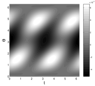
(a)

(b)

Figure 1: Contour plots of (a) $f$ given by Eq. (9) and (b) $f_{2}$ given by Eq. (10) for $\lambda=0.03$ and $\omega_{0}=0.6750$.

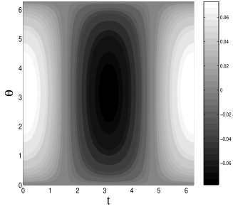
Figure 2: Contour plot of $\lambda J_{0}^{2}v(\theta,t)$ where $v$ is given by Eq. (8) for $\lambda=0.03$ and $\omega_{0}=0.6750$.

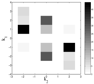
(a)

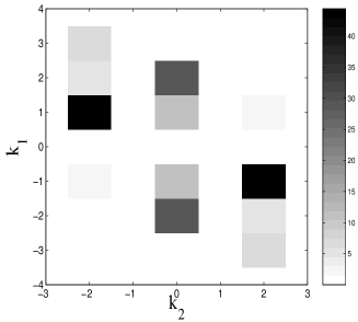
(b)

Figure 3: Two-dimensional Fourier transforms of (a) $f$ given by Eq. (9) and (b) $f_{2}$ given by Eq. (10) for $\lambda=0.03$ and $\omega_{0}=0.6750$.

However, the control terms $f$ and $f_{2}$ given by Eqs. (9) and (10) appear to have a much richer Fourier spectrum. We have represented in Fig. 3 their two-dimensional Fourier transforms. They have an infinite number of Fourier modes and therefore not practical for a numerical or experimental realization. However, it is seen on Fig. 3 that only few Fourier coefficients contribute significantly to the control terms. Therefore, it is feasible to truncate them since the method has been shown to be robust Ciraolo1 . The tailored control term results in general from a trade-off between the ability to control chaos and restrictions on the desired shape for the specific problem at hand.

In order to identify the main Fourier modes, we introduce a parameter $A$ defined as

$$A_{k_{1},k_{2}}\equiv\frac{|f_{k_{1},k_{2}}|}{|k_{1}\omega_{0}+k_{2}|},$$

where $f_{k_{1},k_{2}}$ is the Fourier coefficient with wavevector $(k_{1},k_{2})$ of $f$ or $f_{2}$. The dominant Fourier mode is supposed to have maximal $A$. We notice that this definition contains two effects : First a dominant Fourier mode has to have a significant amplitude, and second, its corresponding wavevector has to be close to a resonance with the frequency vector of the integrable motion (and hence close to a resonance). For $\omega_{0}=0.6750$ (which corresponds to $n_{0}=1$) and $\lambda=0.03$, there is only one dominant Fourier mode in $f$ or $f_{2}$ which has a frequency which is twice the microwave frequency. The truncated control term is given by

$$f_{a}(\theta,t)=f_{3,-2}\cos(3\theta-2t),$$ (13)

where $f_{3,-2}\approx-9.772\times 10^{-4}$ for control term $f$ given by Eq. (9) and $f_{3,-2}\approx-9.739\times 10^{-4}$ for the approximate control term $f_{2}$ given by Eq. (10). We notice that these two values are very close. For this mode, we have $A_{3,-2}\approx 3.90\times 10^{-2}$ which is more than ten times larger than the second largest one $A_{1,-2}\approx 1.90\times 10^{-3}$. We notice that the continued fraction expansion of $\omega_{0}$ is $[0,1,2,\ldots]$. One best approximant is $[0,1,2]=2/3$ which is the frequency of the mode of $f_{a}$.

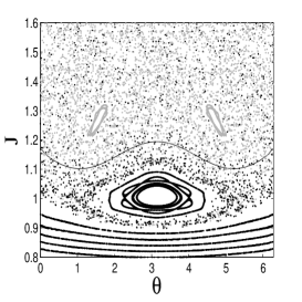
(a)

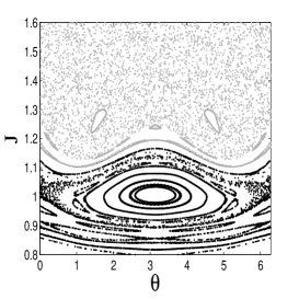
(b)

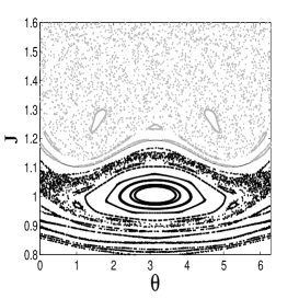
(c)

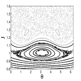
(d)

Figure 4: Poincaré sections of $(a)$ The uncontrolled Hamiltonian $H$ given by Eq. (7), $(b)$ The controlled Hamiltonian $H+f$ where $f$ is given by Eq. (9), $(c)$ The controlled Hamiltonian $H+f_{2}$ where $f_{2}$ is given by Eq. (10), and $(d)$ The controlled Hamiltonian $H+f_{a}$ where $f_{a}$ is given by Eq. (13) for $\lambda=0.03$ and $\omega_{0}=0.6750$. The thin wary curve indicates the location where the invariant torus is restored. The black dots are from trajectories launched below this curve, and gray dots are from trajectories launched above this curve. Note how they are interspersed in $(a)$, as is expected of chaotic trajectories, and how the control restricts their movements in phase space through the invariant torus.

III.2 Poincaré sections

In order to test the efficiency of the control terms to restore invariant tori in phase space, we perform Poincaré sections of $H+f$, $H+f_{2}$ and $H+f_{a}$ and compare them to the Poincaré section of $H$ given by Eq. (7). Since all these Hamiltonians are periodic in time with period $2\pi$, the natural Poincaré section is a stroboscopic plot with period $2\pi$.

Figure 4 depicts Poincaré sections of Hamiltonian (7) in panel $(a)$, Hamiltonian $H+f$ where $f$ is given by Eq. (9) in panel $(b)$, Hamiltonian $H+f_{2}$ where $f_{2}$ is given by Eq. (10) in panel $(c)$ and Hamiltonian $H+f_{a}$ where $f_{a}$ is given by Eq. (13) in panel $(d)$ for $\omega_{0}=0.6750$ and $\lambda=0.03$. We notice that with the addition of the control terms, an invariant torus has been restored which prevent the diffusion from below to above the invariant torus. It is also worth noticing that all of these control terms are efficient although only $f$ is expected to be, indicating that the presence of the control field $f_{2}$ contributes dominantly to a restoration of invariant tori at specific locations such that higher order resonances are eliminated which, in the Chirikov’s approach Chirikov , leads to less chaos and hence less stochastic ionization Cary ; Chandre2 in our problem. It reinforces the robustness of the method and allows one to tailor a control term which is simpler to implement.

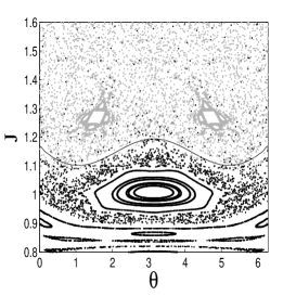
Figure 5: Poincaré sections of Hamiltonian (15) for $\lambda=0.03$ and $\mu=0.0127$.

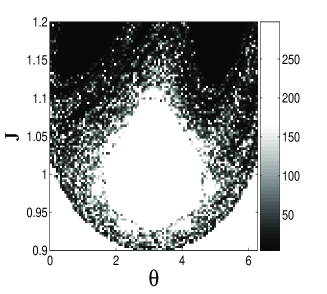
(a)

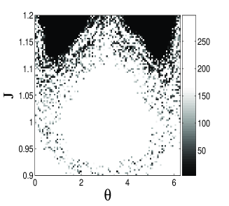
(b)

Figure 6: Laminar plots of $(a)$ Hamiltonian (7) and $(b)$ Hamiltonian (15) for $\lambda=0.03$ and $\mu=0.0127$. Cut-off time is $600\pi$ and diffusion threshold is $J_{th}=1.30$.

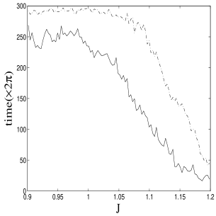
Figure 7: Mean diffusion time $\langle T_{d}\rangle$ versus initial action $J$ with amplitude of external field $\lambda=0.03$. Solid lines are for Hamiltonian (7). Dash-dotted lines are for Hamiltonian (15) for $\mu=0.0127$. Cut-off time is $600\pi$ and diffusion threshold is $J_{th}=1.30$.

III.3 A control term as an additional wave

In Sec. III.1, we show that the frequency of the control wave should be twice the one of the initial wave . Therefore, a possible controlled Hamiltonian is

$$H=\frac{p^{2}}{2}-\frac{1}{x}+\lambda x\cos t+\mu x\cos 2t,$$ (14)

which corresponds to a control terms $g(t)=\mu\cos 2t$ in Eq. (2). In order to obtain the value of $\mu$, we use the Fourier decomposition of the control term $f$ obtained previously. First we map the controlled Hamiltonian into action-angle variables :

$$H=-\frac{1}{2J^{2}}+2J^{2}\left(\lambda\cos t+\mu\cos 2t\right)v(\theta,t),$$ (15)

where $v$ is given by Eq. (8). If we give a value of the action $J_{0}$ where the invariant torus has to be restored, we have seen that the dominant Fourier mode is proportional to $\cos[(2n+1)\theta-2t]$ where $n$ is obtained using the continued fraction expansion of $\omega_{0}=J_{0}^{-3}$. This mode is present in Eq. (15) and has an amplitude given by $\mu J_{0}^{2}a_{2n+1}$. If $f_{2n+1,-2}$ denotes the amplitude of the dominant Fourier mode in Eq. (9) for the values of the parameters $\omega_{0}$ and $\lambda$, then the amplitude of the control field is chosen to be

$$\mu=\frac{f_{2n+1,-2}}{J_{0}^{2}a_{2n+1}}.$$ (16)

The real parameters taken for the external microwave field and control field are flexible for a set of rescaled amplitude of external field $\lambda=0.03$ and frequency $\omega=1$ as long as they satisfy rescaling relationships.

Figure 5 depicts the Poincaré section of the controlled Hamiltonian (15) with $\lambda=0.03$ and $\mu=0.0127$. Figure 5 does not show the restoration of an invariant torus as in the previous cases and hence, the ionization reduction is not obvious. This comes from the fact that the additional wave is quite far from the control term (9) due to additional resonances which break-up the restored invariant torus.

However, the ionization process is still reduced, and this can be seen by looking at laminar plots. Such plots are obtained by looking at a grid of initial conditions and plotting the number of iterations it takes the action to exceed a certain threshold. Figure 6 depicts the laminar plots for Hamiltonian (7) and Hamiltonian (15) with $\lambda=0.03$ and $\mu=0.0127$. The action threshold is chosen to be $J_{th}=1.30$. The maximum integration time is $600\pi$. The darker the region is the smaller time it takes to have $J\geq J_{th}$. It is expected that the laminar plots with more brighter regions are cases where there is less ionization.

In order to compare the diffusion time of trajectories for Hamiltonian (7) with that of the controlled Hamiltonian (15), we have taken a set of N initial angles evenly distributed in $[0,2\pi]$ for one initial action $J$ and then computed the mean diffusion time for each $J$ in both controlled and uncontrolled cases :

$$\langle T_{d}\rangle(J)=\frac{1}{\textsl{N}}\sum_{i=1}^{\textsl{N}}T_{d}(J,\theta_{i}).$$ (17)

Figure 7 depicts the the curve of mean diffusion time $\langle T_{d}\rangle$ versus initial action $J$. In the numerical computation of $T_{d}(J,\theta_{i})$, the integration is performed till the cut-off time $t=600\pi$. Therefore for some trajectories the actual diffusion time is certainly above the cut-off time or even goes to infinity. The double frequency control field also works for the regime $1.14<J<1.20$ for the reason that the rebuilt invariant torus is a curve which goes beyond $J_{0}=\omega_{0}^{-1/3}=1.14$ for some areas. Figure 7 shows that the mean diffusion time for controlled Hamiltonian (15) is significantly larger than that for Hamiltonian (7) which clearly shows the effect of the additional microwave field to reduce ionization.

IV Conclusion

In this paper we implemented a local control method on the one-dimensional hydrogen atom in a linearly polarized (LP) microwave field in order to reduce ionization. After simplifying the originally complicated control function numerically, we obtained an extremely simple control term which is in the same form as the external LP microwave field but with smaller amplitude. Adding the small control field to the perturbed Hamiltonian leads to a reduction of ionization. We have done the calculations in a regime where the quantum and classical agree, and our classical computations show efficient suppression of ionization. Preliminary results we obtained for controlling ionization in higher dimensions show the promise of the local control method for manipulating ionization in full-dimensional Rydberg atoms and work in this direction is currently under way in our center.

- (1) T. F. Gallagher, Rydberg Atoms (Cambridge University Press, Cambridge, UK, 1994)
- (2) J.E. Bayfield and P.M. Koch, Phys. Rev. Lett. 33, 258 (1974)
- (3) J.-P. Connerade, Highly Excited Atoms (Cambridge University Press, Cambridge, UK, 1998)
- (4) P. M. Koch and K. A. H. van Leeuwen, Phys. Rep. 255, 289 (1995)
- (5) G. Casati, B.V. Chirikov, I. Guarneri, D.L. Shepelyansky, Phys. Rep. 154, 77 (1987)
- (6) G. Casati, I. Guarneri, and D.L. Shepelyansky, IEEE J. Quantum Electron. 24, 1420 (1988)
- (7) R. V. Jensen, Phys. Rep. 201, 1 (1991)
- (8) B.I. Meerson, E.A. Oks and P.V. Sasorov, Pis’ma Zh. Eksp. Teor. Fiz. 29, 79 (1979) [JETP Lett. 29, 72 (1979)]
- (9) J.G. Leopold and I.C Percival, J. Phys. B 12, 709 (1979)
- (10) R. V. Jensen, Phys. Rev. A 30, 386 (1984)
- (11) R. S. MacKay and J. D. Meiss, Phys. Rev. A 37, 4702 (1988)
- (12) D. Farrelly and T. Uzer, Phys. Rev. A, 38, 5902 (1988)
- (13) J.E. Howard, Phys. Lett. A 156, 286 (1991)
- (14) J.E. Howard, Phys. Rev. A 46, 1 (1992)
- (15) L.E. Reichl, The Transition to Chaos in Conservative Classical Systems: Quantum Manifestations (Springer-Verlag, New York, 1992)
- (16) R. Blümel and W. P. Reinhardt, Chaos in Atomic Physics (Cambridge University Press, Cambridge, UK, 1997)
- (17) A. Buchleitner, D. Delande and J.-C. Gay, J. Opt. Soc. Am. B 12, 505 (1995)
- (18) A. Krug and A. Buchleitner, Phys. Rev. A 72, 061402(R) (2005)
- (19) M.V. Berry, Proc. R. Soc. Lond. A 413, 183 (1987)
- (20) J.G. Leopold and D. Richards, J. Phys. B 18, 3369 (1985)
- (21) J.G. Leopold and D. Richards, J. Phys. B 22, 131 (1989)
- (22) R. Blümel and U. Smilansky, Phys. Scr. 40, 386 (1989)
- (23) D. Delande, Chaos in atomic and molecular physics, in: M. J. Giannoni, A. Voros, J. Zinn-Justin(Eds), Chaos and Quantum Physics, Les Houches, Session LII, 1989, Elsevier, Amsterdam, 1991, p.665
- (24) L. Perotti, Phys. Rev. A 73, 053405 (2006)
- (25) L. Ko, M. W. Noel, J. Lambert and T. F. Gallagher, J. Phys. B 32, 3469 (1999)
- (26) L. Sirko, S. A. Zelazny, and P. M. Koch, Phy. Rev. Lett. 87, 043002 (2001)
- (27) L. Sirko and P. M. Koch, Phy. Rev. Lett. 89, 274101 (2002)
- (28) P. M. Koch, S. A. Zelazny and L. Sirko, J. Phys. B: At. Mol. Opt. Phys. 36, 4755 (2003)
- (29) H. Maeda and T. F. Gallagher, Phy. Rev. Lett. 93, 193002 (2004)
- (30) H. Maeda, J. H. Gurian, D. V. L. Norum and T. F. Gallagher, Phys. Rev. Lett. 96, 073002 (2006)
- (31) T. Prosen and D. L. Shepelyansky, Eur. Phys. J. B 46, 515 (2005)
- (32) C. Chandre, M. Vittot, G. Ciraolo, Ph. Ghendrih and R. Lima, Nucl. Fusion 46, 33 (2006)
- (33) B.V. Chirikov, Phys. Rep. 52, 263 (1979)
- (34) G. Ciraolo, C. Chandre, R. Lima, M. Vittot, M. Pettini, C. Figarella and P. Ghendrih, J. Phys. A: Math. Gen. 37, 3589 (2004)
- (35) G. Casati, B. V. Chirikov, D. L. Shepelyansky, and I. Guarneri, Phys. Rev. Lett. 57, 823 (1986)
- (36) E. J. Galvez, B. E. Sauer, L. Moorman, P. M. Koch, and D. Richards, Phys. Rev. Lett. 61, 2011 (1988)
- (37) J. R. Cary and J. D. Hanson, Phys. Fluids 29, 2464 (1986)