Moving solitons in the discrete nonlinear Schrödinger equation

Abstract

Using the method of asymptotics beyond all orders, we evaluate the amplitude of radiation from a moving small-amplitude soliton in the discrete nonlinear Schrödinger equation. When the nonlinearity is of the cubic type, this amplitude is shown to be nonzero for all velocities and therefore small-amplitude solitons moving without emitting radiation do not exist. In the case of a saturable nonlinearity, on the other hand, the radiation is found to be completely suppressed when the soliton moves at one of certain isolated ‘sliding velocities’. We show that a discrete soliton moving at a general speed will experience radiative deceleration until it either stops and remains pinned to the lattice, or—in the saturable case—locks, metastably, onto one of the sliding velocities. When the soliton’s amplitude is small, however, this deceleration is extremely slow; hence, despite losing energy to radiation, the discrete soliton may spend an exponentially long time travelling with virtually unchanged amplitude and speed.

I Introduction

This paper deals with moving solitons of the discrete nonlinear Schrödinger (DNLS) equation. The earliest applications of the cubic DNLS equation were to the self-trapping of electrons in lattices (the polaron problem) and energy transfer in biological chains (Davydov solitons) – see the reviews hennig ; braun ; scott for references. Relatedly, the equation arises in the description of small-amplitude breathers in Frenkel-Kontorova chains with weak coupling braun . In optics the equation describes light-pulse propagation in nonlinear waveguide arrays in the tight-binding limit christodoulides ; campbell . Most recently the DNLS equation has been used to model Bose-Einstein condensates in optically induced lattices trambettoni .

The question of the existence of moving solitons in the DNLS equation has been the subject of debate for some time duncan ; flach ; eilbeck ; ablowitz ; Kundu ; pelinovsky ; kevrekidis ; Feddersen ; FKZ ; Flach_Kladko ; Malomed_collisions_1 ; Malomed_collisions_2 ; Malomed_nonlinearity_management . Recently, Gómez-Gardeñes, Floría, Falo, Peyrard and Bishop gomez1 ; gomez have demonstrated that the stationary motion of pulses in the cubic one-site DNLS (the ‘standard’ DNLS) is only possible over an oscillatory background consisting of a superposition of plane waves. This result was obtained by numerical continuation of the moving Ablowitz-Ladik breather with two commensurate time scales. In our present paper, we study the travelling discrete solitons analytically and independently of any reference models. Consistently with the conclusions of gomez1 ; gomez , we will show that solitons cannot freely move in the cubic DNLS equation; they emit radiation, decelerate and eventually become pinned by the lattice. We shall show, however, that this radiation is exponentially small in the soliton’s amplitude, so that broad, small-amplitude pulses are highly mobile and are for all practical purposes indistinguishable from freely moving solitons.

In the context of optical waveguide arrays—important not only in themselves but also as a first step to understanding more complicated optical systems such as photonic crystals—interest among experimentalists efremidis ; fleischer ; chen has recently shifted away from media with pure-Kerr nonlinearity (which gives rise to a cubic term in the DNLS equation) and towards photorefractive media, which exhibit a saturable nonlinearity cuevas ; fleischer-nature ; vicencio ; hadzievski ; stepic . In practice such arrays may be optically induced in a photorefractive material efremidis ; fleischer or fabricated permanently – see chen , for example. The study of solitons in continuous optical systems with saturable nonlinearitites has a long history; interesting phenomena here include bistability gatz1 ; gatz2 , fusion tikhonenko and radiation effects vidal which do not arise in the cubic equation. As for the discrete case, the work of Khare, Rasmussen, Samuelsen and Saxena khare suggests that the saturable one-site DNLS may be exceptional in the sense of ref. BOP ; that is, despite not being a translation invariant system, it supports translationally invariant stationary solitons. This property is usually seen as a prerequisite for undamped motion in discrete equations (see e.g. OPB ) and indeed, the numerical experiments of Vicencio and Johansson vicencio have revealed that soliton mobility is enhanced in the saturable DNLS equation.

The DNLS equation with a saturable nonlinearity is the second object of our analysis here; our conclusions will turn out to be in agreement with the numerical observations of ref. vicencio . We will show that for nonlinearities which saturate at a low enough intensity, solitons can slide—that is, move without radiative deceleration—at certain isolated velocities. These ‘sliding’ solitons are examples of embedded solitons.

The usual saturable DNLS equation is the discrete form of the Vinetskii-Kukhtarev model vinetskii :

$$i\dot{\Phi}_{n}+\Phi_{n+1}-2\Phi_{n}+\Phi_{n-1}-\gamma\frac{1}{1+|\Phi_{n}|^{2}}\Phi_{n}=0.$$ (1)

In order to encompass both cubic and saturable nonlinearities in a single model, we shall instead consider the equation

$$i\dot{\phi}_{n}+\phi_{n+1}+\phi_{n-1}+\frac{2|\phi_{n}|^{2}}{1+\mu|\phi_{n}|^{2}}\phi_{n}=0,$$ (2)

obtained from eq. (1) by making the transformation $\Phi_{n}=\sqrt{2/\gamma}e^{-i(2+\gamma)t}\phi_{n}$ and letting $\mu=2/\gamma$. In the form above, $1/\mu$ represents the saturation threshold of the medium gatz2 , which tends to infinity as one approaches the pure Kerr (cubic) case of $\mu=0$. The higher the value of $\mu$, the lower is the intensity at which the nonlinearity saturates.

This paper is structured in the following way. In section II, we construct a small-amplitude, broad travelling pulse as an asymptotic series in powers of $\epsilon$, its amplitude. The velocity and frequency of this soliton are obtained as explicit functions of $\epsilon$ and its carrier-wave wavenumber. Then in section III, the main section of this paper, we derive an expression for the soliton’s radiation tails and measure their amplitude using the method of asymptotics beyond all orders. In section IV, we investigate the influence of this exponentially weak radiation on the soliton’s amplitude and speed. Finally, in section V, we summarise our work and make comparisons with some earlier results.

II Asymptotic Expansion

II.1 Leading order

We begin by seeking solutions of the form

$$\phi_{n}(t)=\psi(X)e^{ikn+i\omega t},$$ (3)

where

$$X=\epsilon(n-vt)$$ (4)

and $\epsilon$ is a parameter. By analogy with the soliton of the continuous NLS, we expect the discrete soliton to be uniquely characterised by two parameters—e.g. $\epsilon$ and $k$—while the other two ($\omega$ and $v$) are expected to be expressible through $\epsilon$ and $k$. Substituting the Ansatz (3), (4) into (2) gives a differential advance-delay equation

$$\psi(X+\epsilon)e^{ik}+\psi(X-\epsilon)e^{-ik}-\omega\psi(X)\\ -i\epsilon v\psi^{\prime}(X)+\frac{2|\psi(X)|^{2}}{1+\mu|\psi(X)|^{2}}\psi(X)=0.$$ (5)

This can be written as an ordinary differential equation of an infinite order:

$$e^{ik}\sum_{n=0}^{\infty}\epsilon^{n}\frac{1}{n!}\psi^{(n)}+e^{-ik}\sum_{n=0}^{\infty}\epsilon^{n}\frac{(-1)^{n}}{n!}\psi^{(n)}-\omega\psi\\ -i\epsilon v\psi^{\prime}+\frac{2|\psi|^{2}}{1+\mu|\psi|^{2}}\psi=0,$$ (6)

where $\psi^{(n)}=d^{n}\psi/dX^{n}$.

From now on we assume that $\epsilon$ is small. Our aim in this section is to find an approximate solution to eq. (6)—and hence eq. (2)—with $\psi={\cal O}(\epsilon)$. (That is, we are looking for small, broad pulses which modulate a periodic carrier wave.) To this end, we expand $\psi$, $\omega$ and $v$ as power series in $\epsilon$:

$$\psi =\epsilon(\psi_{0}+\epsilon\psi_{1}+\cdots),$$ (7a)

$$\omega =\omega_{0}+\epsilon^{2}\omega_{2}+\cdots,$$ (7b)

$$v =v_{0}+\epsilon^{2}v_{2}+\cdots.$$ (7c)

(We are not expanding $k$ as we consider it, along with $\epsilon$, as one of the two independent parameters characterising our solution.) Substituting these expansions into eq. (6) gives a hierarchy of equations to be satisfied at each power of $\epsilon$ by choosing $\omega_{n}$ and $v_{n}$ properly. In nonlinear oscillations, this perturbation procedure is known as Lindstedt’s method Lindstedt .

At the order $\epsilon^{1}$ we obtain

$$\omega_{0}=2\cos k,$$ (8)

while the order $\epsilon^{2}$ gives

$$v_{0}=2\sin k.$$ (9)

These two relations correspond to the dispersion of linear waves. At the power $\epsilon^{3}$ we obtain the following nonlinear equation for $\psi_{0}$:

$$\cos k\,\psi^{\prime\prime}_{0}-\omega_{2}\psi_{0}+2|\psi_{0}|^{2}\psi_{0}=0.$$

This is the stationary form of the NLS equation, which has the homoclinic solution

$$\psi_{0}=a\sqrt{\cos k}\operatorname{sech}(aX)$$

with

$$a^{2}=\frac{\omega_{2}}{\cos k}.$$

Returning to the original variable $\psi$, we note that the amplitude $a$ can always be absorbed into $\epsilon$, the parameter in eq. (4) and in front of $\psi_{0}$ in (7a). That is, there is no loss of generality in setting $a=1$ and letting $\epsilon$ describe the amplitude (and inverse width) of the pulse instead. This allows us to set

$$\omega_{2}=\cos k.$$ (10)

Note that the coefficients in eq. (5) are periodic functions of the parameter $k$ with period $2\pi$; therefore it is sufficient to consider $k$ in the interval $(-\pi,\pi)$. Also, (5) is invariant with respect to the transformation $k\rightarrow-k$, $\epsilon\rightarrow-\epsilon$, $v\rightarrow-v$; hence it is sufficient to consider positive $k$ only. Finally, our perturbative solution does not exist if $\cos k$ is negative. Thus, from now on we shall assume that $0\leq k\leq\pi/2$.

II.2 Higher orders

At the order $\epsilon^{n+3}$, where $n\geq 1$, we arrive at the following equations for the real and imaginary parts of $\psi_{n}$:

$${\cal L}_{1}\operatorname{Re}\psi_{n} =\frac{\operatorname{Re}f_{n-1}(X)}{\cos k}$$ (11a)

$${\cal L}_{0}\operatorname{Im}\psi_{n} =\frac{\operatorname{Im}f_{n-1}(X)}{\cos k},$$ (11b)

where

$${\cal L}_{0} =-d^{2}/dX^{2}+1-2\operatorname{sech}^{2}X,$$

$${\cal L}_{1} =-d^{2}/dX^{2}+1-6\operatorname{sech}^{2}X$$

and

$$f_{n-1}(X)=\sum_{j=1}^{[n/2]}\left(\frac{2\cos k}{(2j+2)!}\psi_{n-2j}^{(2j+2)}-\omega_{2j+2}\psi_{n-2j}\right)+i\sum_{j=1}^{[\frac{n+1}{2}]}\left(\frac{2\sin k}{(2j+1)!}\psi_{n-2j+1}^{(2j+1)}-v_{2j}\psi^{\prime}_{n-2j+1}\right)\\ +\sum_{m=1}^{n-1}2\psi_{0}(\psi_{m}{\psi}^{\ast}_{n-m}-\psi_{n-m}{\psi}^{\ast}_{m})+\sum_{m=1}^{n-1}\sum_{\ell=0}^{n-1-m}2\psi_{n-m-\ell}\psi_{m}{\psi}^{\ast}_{\ell}\\ +\mu\sum_{m=0}^{n-1}\sum_{\ell=0}^{n-1-m}\Bigg{[}\sum_{j=1}^{[\frac{n-m-\ell}{2}]}\left(\frac{2\cos k}{(2j)!}\psi^{(2j)}_{n-m-\ell-2j}-\omega_{2j}\psi_{n-m-\ell-2j}\right)\\ +i\sum_{j=1}^{[\frac{n-m-\ell-1}{2}]}\left(\frac{2\sin k}{(2j+1)!}\psi^{(2j+1)}_{n-m-\ell-2j-1}-v_{2j}\psi^{\prime}_{n-m-\ell-2j-1}\right)\Bigg{]}\psi_{m}{\psi}^{\ast}_{\ell}.$$ (12)

The linear nonhomogeneous ordinary differential equations (11) must be solved subject to a boundedness condition.

The bounded homogeneous solutions of eqs (11a) and (11b) ($\operatorname{sech}X\tanh X$ and $\operatorname{sech}X$, respectively) correspond to the translation- and U(1)-invariances of eq. (5). Including these zero modes in the full solution of eqs (11) would amount just to the translation of $\psi(X)$ by a constant distance in $X$ and its multiplication by a constant phase factor. These deformations are trivial, and hence we can safely discard the homogeneous solutions at each order of $\epsilon$.

As $\psi_{0}$’s real part is even and its imaginary part is odd (zero), $\psi_{1}$’s real and imaginary parts are also even and odd, respectively. The same holds, by induction, to all orders of the perturbation theory. Indeed, assume that $\psi_{0},\psi_{1},\ldots,\psi_{n-1}$ have even real parts and odd imaginary parts. Then it is not difficult to verify that the function ${\rm Re}f_{n-1}(X)$ is even and ${\rm Im}f_{n-1}(X)$ is odd. Since the operators ${\cal L}_{0}$ and ${\cal L}_{1}$ are parity-preserving, and since we have excluded the corresponding homogeneous solutions, this means that $\psi_{n}$ has an even real part and an odd imaginary part. Finally, the homogeneous solution of (11b) being even and that of (11a) being odd, the corresponding solvability conditions are satisfied at any order.

Note that since the solvability conditions do not impose any constraints on $v_{n}$ and $\omega_{n}$, the coefficients $v_{n}$ with $n\geq 2$ and $\omega_{n}$ with $n\geq 4$ can be chosen completely arbitrarily.

II.3 Explicit perturbative solution to order $\epsilon^{3}$

Solving eqs (11) successively, we can obtain the discrete soliton (7a) to any desired accuracy. Here, we restrict ourselves to corrections up to the cubic power in $\epsilon$. The order $\epsilon^{3}$ is the lowest order at which the saturation parameter $\mu$ appears in the solution. On the other hand, it is high enough to exemplify and motivate our choice of the coefficients in (7b) and (7c).

Letting $n=1$ in eq. (12), we have

$$f_{0}(X)=\frac{2i}{3!}\sin k\psi_{0}^{\prime\prime\prime}-iv_{2}\psi^{\prime}_{0}.$$

The corresponding solution of eq. (11) is

$$\psi_{1}=\, \frac{i}{\sqrt{\cos k}}\Bigg{[}\frac{1}{2}\sin k\operatorname{sech}X\tanh X$$

$$\;\;\;\;+\frac{1}{2}\left(v_{2}-\frac{1}{3}\sin k\right)X\operatorname{sech}X\Bigg{]}.$$

Here the term proportional to $X\operatorname{sech}X$ decays to zero as $|X|\to\infty$; however, it becomes greater than $\psi_{0}(X)$ for sufficiently large $|X|$, leading to nonuniformity of the expansion (7a). In order to obtain a uniform expansion, the term in question should be eliminated. Being free to choose the coefficients $v_{n}$ with $n\geq 2$, we use this freedom to set

$$v_{2}=\frac{1}{3}\sin k.$$

This leaves us with

$$\psi_{1}=\frac{i}{2}\sqrt{\cos k}\tan k\operatorname{sech}X\tanh X.$$

After ‘distilling’ in a similar way the correction $\psi_{2}$, where we fix

$$\omega_{4}=\frac{1}{12}\cos k$$

to eliminate a term proportional to $X\operatorname{sech}X$, we obtain

$$\psi =\epsilon\sqrt{\cos k}\Big{\{}\operatorname{sech}X+\frac{i}{2}\epsilon\tan k\operatorname{sech}X\tanh X$$

$$\;\;+\frac{1}{12}\epsilon^{2}\big{[}4\operatorname{sech}^{3}X-3\operatorname{sech}X$$

$$\;\;\;\;+\frac{1}{2}\tan^{2}k(14\operatorname{sech}^{3}X-13\operatorname{sech}X)$$

$$\;\;\;\;\;\;+4\mu\cos k(2\operatorname{sech}X-\operatorname{sech}^{3}X)\big{]}+{\cal O}(\epsilon^{3})\Big{\}},$$ (13)

where

$$\omega =2\left[1+\frac{1}{2!}\epsilon^{2}+\frac{1}{4!}\epsilon^{4}+{\cal O}(\epsilon^{6})\right]\cos k,$$ (14a)

$$v =2\left[1+\frac{1}{3!}\epsilon^{2}+{\cal O}(\epsilon^{4})\right]\sin k.$$ (14b)

II.4 Velocity and frequency of the discrete soliton

In the previous subsection we have shown that fixing suitably the coefficients $\omega_{n}$ and $v_{n}$ can lead to a uniform expansion of $\psi$ to order $\epsilon^{3}$. Our approach was based on solving for $\psi_{n}$ explicitly and then setting the coefficients in front of the ‘secular’ terms $X\operatorname{sech}X$ to zero. Here, we show that the secular terms can be eliminated to all orders – and without appealing to explicit solutions.

Assume that the secular terms have been suppressed in all nonhomogeneous solutions $\psi_{m}$ with $m$ up to $n-1$; that is, let

$$\psi_{m}(X) \to C_{m}e^{X}+o(e^{X})$$

$$\quad\mbox{as}\ X\to-\infty\quad(m=0,1,\ldots,n-1).$$ (15)

(Since we know that the real part of $\psi_{m}$ is even and the imaginary part odd, it is sufficient to consider the asymptotic behaviour at one infinity only.) The constant $C_{m}$ may happen to be zero for some $m$ in which case the decay of $\psi_{m}$ will be faster than $e^{X}$. Our objective is to choose $\omega_{n}$ and $v_{n}$ in such a way that $\psi_{n}(X)$ will also satisfy (15). To this end, we consider the function (12). All terms which are trilinear in $\psi_{0},\ldots,\psi_{n-1}$ and derivatives of these functions decay as $e^{3X}$ or faster; these terms in $f_{n-1}$ cannot give rise to the secular terms proportional to $X\operatorname{sech}X$ in $\psi_{n}$. On the other hand, the terms making up the first line in (12) tend to

$$e^{X}\sum_{j=1}^{[n/2]}\left[\frac{2\cos k}{(2j+2)!}-\omega_{2j+2}\right]C_{n-2j}$$

$$\quad+ie^{X}\sum_{j=1}^{[\frac{n+1}{2}]}\left[\frac{2\sin k}{(2j+1)!}-v_{2j}\right]C_{n-2j+1}$$

as $X\to-\infty$. These are ‘asymptotically resonant’ terms – in the sense that their asymptotics are proportional to the asymptotics of the homogeneous solutions of (11a) and (11b). It is these terms on the right-hand sides of (11a) and (11b) that give rise to the secular terms in the solution $\psi_{n}$. The resonant terms will be suppressed if we let

$$\omega_{2j+2}=\frac{2\cos k}{(2j+2)!},\quad v_{2j}=\frac{2\sin k}{(2j+1)!},\quad j\geq 1.$$ (16)

After the resonant terms have been eliminated, the bounded solution to (11) will have the asymptotic behaviour $\psi_{n}\to C_{n}e^{X}$ as $X\to-\infty$. By induction, this result extends to all $n\geq 0$.

Substituting (16), together with (8)–(10), into eqs (7b) and (7c), and summing up the series, we obtain

$$\omega=2\cos k\cosh\epsilon,\quad v=2\sin k\frac{\sinh\epsilon}{\epsilon},$$ (17)

the frequency and velocity of the discrete soliton parameterised in terms of $k$ and $\epsilon$.

Equations (17) coincide with the expressions AL of the Ablowitz-Ladik soliton’s velocity and frequency in terms of its amplitude and wavenumber. The difference between the two sets of answers is in that eqs (17) pertain to small-amplitude solitons only, whereas Ablowitz and Ladik’s formulas are valid for arbitrarily large amplitudes.

Note, also, that the velocity and frequency (17) do not depend on the saturation parameter $\mu$. This is in contrast to the stationary ($v=0$) soliton of eqs (5) and (6) obtained by Khare, Rasmussen, Samuelsen and Saxena khare . The soliton of ref. khare has its amplitude and frequency uniquely determined by $\mu$.

III Terms beyond all orders of the perturbation theory

III.1 Dispersion relation for linear waves

As $X\to-\infty$, the series (7a) reduces to $\psi(X)=\sum_{n=0}^{\infty}\epsilon^{n+1}C_{n}e^{X}$. The convergence of the series $\sum\epsilon^{n+1}\psi_{n}(X)$ for all $X$ would imply, in particular, the convergence of the series $\sum\epsilon^{n+1}C_{n}$. Therefore, if the series (7a) converged, the solution $\psi(X)$ would be decaying to zero as $X\to-\infty$. However, although we have shown that the series $\sum\epsilon^{n+1}\psi_{n}(X)$ is asymptotic to all orders, it does not have to be convergent. For instance, it is easy to see that the series cannot converge for $v=\mu=0$ and any $\epsilon$; since the advance-delay equation (5) is translation invariant, this would imply that we have constructed a family of stationary solitons with an arbitrary position relative to the lattice. This, in turn, would contradict the well established fact that the ‘standard’ cubic DNLS solitons can only be centered on a site or midway between two adjacent sites Laedke_Kluth_Spatschek (that is, that the ‘standard’ discretisation of the cubic NLS is not exceptional pelinovsky-exceptional ). Thus, we expect that the perturbative solution (7a) satisfies $\psi(X)\to 0$ as $|X|\to\infty$ only for some special choices of $v$, $\epsilon$ and $\mu$.

Can eqs (5) and (6) have a bounded solution despite the divergence of the corresponding series $\sum\epsilon^{n+1}C_{n}$? To gain some insight into this matter, we linearise eq. (5) about $\psi=0$ and find nondecaying solutions of the form $\psi=e^{i{\cal Q}X/\epsilon}$ where ${\cal Q}$ is a root of the dispersion relation

$$\omega=2\cos(k+{\cal Q})+{\cal Q}v.$$ (18)

It is easy to check that there is at least one such harmonic solution [i.e. eq. (18) has at least one root] if $v\neq 0$. These harmonic waves can form a radiation background over which the soliton propagates (as suggested by the numerics of gomez1 ; gomez and the analysis of a similar problem for the $\phi^{4}$ kinks in OPB ). Being nonanalytic in $\epsilon$, such backgrounds cannot be captured by any order of the perturbation expansion.

As we will show below, not only the wavenumbers but also the amplitudes of the harmonic waves are nonanalytic in $\epsilon$. This phenomenon was first encountered in the context of the breather of the continuous $\phi^{4}$ model, where Eleonskii, Kulagin, Novozhilova, and Silin eleonskii suggested that the radiation from the breather could be exponentially weak. Segur and Kruskal sk ; sk2 then developed the method of ‘asymptotics beyond all orders’ to demonstrate that, in the limit $\epsilon\rightarrow 0$, such radiation does exist. We will use Segur and Kruskal’s method to measure the magnitude of the radiation background of the travelling discrete soliton.

Qualitatively, the fact that the radiation is not excited at any order of the perturbation expansion is explained by the fact that the soliton exists on the long length scale $X$, whereas the radiation has the shorter scale $X/\epsilon$. To all orders, the two are uncoupled.

Using the relations (17), we can rewrite (18) as

$$\frac{\cosh\epsilon-\cos{\cal Q}}{(\sinh\epsilon/\epsilon){\cal Q}-\sin{\cal Q}}=\tan k.$$ (19)

The left hand side is plotted in fig. 1. For $\epsilon=0$ it has minima at multiples of $2\pi$ where the curve is tangent to the horizontal axis. For nonzero $\epsilon$, the minima of the curve are lifted off the ${\cal Q}$ axis slightly. The minima with larger values of ${\cal Q}$ have smaller elevations above the horizontal axis; i.e., the minima come closer and closer to the ${\cal Q}$ axis as ${\cal Q}$ grows. We see from the figure that for $k>k^{(1)}_{\rm max}$, where $k^{(1)}_{\rm max}\approx 0.22$, there is only one radiation mode. Note also that the left-hand side of eq. (19) is negative for negative ${\cal Q}$; since we have assumed that $0\leq k\leq\pi/2$, this implies that eq. (19) cannot have negative roots.

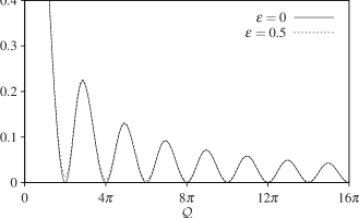
Figure 1: The left hand side of eq. (19) for two values of $\epsilon$. The root(s) ${\cal Q}_{n}$ of the dispersion relation (18) are located where this graph is intersected by a horizontal straight line with ordinate equal to $\tan k$.

III.2 Radiating solitons

Although we originally constructed the expansion (7a) as an asymptotic approximation to a solution which is stationary in the frame of reference moving with the velocity $v$, it can also represent an approximation to a time-dependent solution $\psi(X,t)$. Here $\psi(X,t)$ is related to $\phi_{n}(t)$, the discrete variable in eq. (2), by the substitution (3):

$$\phi_{n}(t)=\psi(X,t)e^{ikn+i\omega t}.$$ (20)

The coefficients $\psi_{n}$ in the asymptotic expansion of $\psi(X,t)$ will coincide with the coefficients in the expansion of the stationary solution $\psi(X)=\sum\epsilon^{n+1}\psi_{n}$ if the time derivatives $\partial_{t}\psi_{n}$ lie beyond all orders of $\epsilon$ and hence the time evolution of the free parameters $k$ and $\epsilon$ occurs on a time scale longer than any power of $\epsilon^{-1}$. Physically, one such solution represents a travelling soliton slowing down and attenuating as the Cherenkov radiation left in its wake carries momentum and energy away from its core.

Substituting (20) into eq. (2), gives

$$i\psi_{t}+\psi^{+}e^{ik}+\psi^{-}e^{-ik}-\omega\psi-i\epsilon v\psi_{X}+\frac{2|\psi|^{2}}{1+\mu|\psi|^{2}}\psi=0,$$ (21)

where $\psi^{\pm}=\psi(X\pm\epsilon,t)$.

We consider two solutions of this equation which both have the same asymptotic expansion (7a), denoted $\psi_{s}(X,t)$ and $\psi_{u}(X,t)$, such that $\psi_{s}(X,t)\to 0$ as $X\to+\infty$ and $\psi_{u}(X,t)\to 0$ as $X\to-\infty$. Since the difference $\Psi\equiv\psi_{s}-\psi_{u}$ is small (lies beyond all orders of $\epsilon$), and since the solution $\psi_{s}$ can be regarded as a perturbation of $\psi_{u}$, $\Psi$ obeys the linearisation of eq. (21) about $\psi_{u}$ to a good approximation. That is,

$$i\Psi_{t}+\Psi^{+}e^{ik}+\Psi^{-}e^{-ik}-\omega\Psi-iv\epsilon\Psi_{X}\\ +\frac{4|\psi_{u}|^{2}\Psi+2\psi_{u}^{2}{\Psi}^{\ast}}{1+\mu|\psi_{u}|^{2}}+\frac{2\mu|\psi_{u}|^{2}(|\psi_{u}|^{2}\Psi+\psi_{u}^{2}{\Psi}^{\ast})}{(1+\mu|\psi_{u}|^{2})^{2}}=0.$$ (22)

Since $\psi_{u}={\cal O}\left({\epsilon}\right)$, we can solve eq. (22) to leading order in $\epsilon$ by ignoring the last two terms in it; the resulting solutions are exponentials of the form $e^{i\mathcal{Q}X/\epsilon-i\Omega t}$. We make a preemptive simplification by setting $\Omega=0$. [That $\Omega$ has to be set equal to zero follows from matching these exponentials to the far-field asymptotes of the stationary ‘inner’ solution; see section III.4 below. Physically, $\Omega=0$ implies that the travelling pulse will only excite the radiation with its own (zero) frequency in the comoving frame.] The leading-order solution of eq. (22) is therefore

$$\Psi=\sum_{n}A_{n}e^{i{\cal Q}_{n}X/\epsilon}+{\cal O}\left({\epsilon^{1}}\right),$$ (23)

where ${\cal Q}_{n}$ ($n=1,2,\ldots$) are the roots, numbered in order from smallest to largest, of the dispersion relation (18). (Recall that since we have taken $k$ in the interval $[0,\pi/2]$, all the roots ${\cal Q}_{n}$ are positive.) For $k>k_{\rm max}^{(1)}\approx 0.22$, there is only one root, ${\cal Q}_{1}$.

Higher-order corrections to the solution (23) can be found by substituting the ansatz

$$\Psi=\sum_{n}A_{n}[1+\epsilon f_{1}^{(n)}(X)+\epsilon^{2}f_{2}^{(n)}(X)+\cdots]e^{i{\cal Q}_{n}X/\epsilon}\\ +\sum_{n}A_{n}^{*}[\epsilon^{2}g_{2}^{(n)}(X)+\epsilon^{3}g_{3}^{(n)}(X)+\cdots]e^{-i{\cal Q}_{n}X/\epsilon}$$ (24)

into eq. (22), expanding the advance/delay terms $f^{(n)}_{1,2,\ldots}(X\pm\epsilon)$ and $g^{(n)}_{2,3,\ldots}(X\pm\epsilon)$ in Taylor series in $\epsilon$, and making use of the asymptotic expansion (7a), (II.3) for $\psi_{u}$. For instance, the first few corrections are found to be

$$\begin{split}f_{1}^{(n)}(X)&=\frac{4i\cos k}{2\sin(k+{\cal Q}_{n})-v}\tanh X,\\ g_{2}^{(n)}(X)&=\frac{2\cos k}{\omega+vq_{n}-2\cos(k-{\cal Q}_{n})}\operatorname{sech}^{2}X.\end{split}$$ (25)

Since $\psi_{u}\to 0$ as $X\to-\infty$, it follows that $\psi_{s}\to\Psi$ as $X\to-\infty$, and hence, once we know the amplitudes $A_{n}$, we know the asymptotic behaviour of $\psi_{s}$. We shall now employ the method of asymptotics beyond all orders to evaluate these amplitudes.

III.3 ‘Inner’ equations

Segur and Kruskal’s method allows one to measure the amplitude of the exponentially small radiation by continuing the solution analytically into the complex plane. The leading-order term of $\psi$, $\epsilon\sqrt{\cos k}\operatorname{sech}X$, has singularities at $X=\frac{i\pi}{2}+i\pi n$, $n=0,\pm 1,\pm 2,\ldots$. In the vicinity of these points, the radiation becomes significant; the qualitative explanation for this is that the $\operatorname{sech}$ function forms a sharp spike with a short length scale near the singularity point, and hence there is a strong coupling to the radiation modes, unlike on the real axis. The radiation, which is exponentially small on the real axis, becomes large enough to be measured near the singularities.

We define a new complex variable $y$, such that $\epsilon y$ is small in absolute value when $X$ is near the lowest singularity in the upper half-plane:

$$\epsilon y=X-\frac{i\pi}{2}.$$ (26)

The variables $y$ and $X$ are usually referred to as the ‘inner’ and ‘outer’ variables, respectively – the transformation to $y$ effectively ‘zooms in’ on the singularity at $X=\frac{i\pi}{2}$. We also define $u(y)\equiv\psi(X)$ and $w(y)\equiv\psi^{*}(X)$. Continuing eq. (5) to the complex plane—i.e. substituting $u(y)$ for $\psi(X)$ and $w(y)$ for $\psi^{*}(X)$—we obtain, in the limit $\epsilon\to 0$,

$$e^{ik}u(y+1)+e^{-ik}u(y-1)-2\cos k\,u(y)-2i\sin k\,u^{\prime}(y)+\frac{2u^{2}w}{1+\mu uw}=0,$$ (27a)

$$e^{-ik}w(y+1)+e^{ik}w(y-1)-2\cos k\,w(y)+2i\sin k\,w^{\prime}(y)+\frac{2w^{2}u}{1+\mu wu}=0.$$ (27b)

Here we have used the fact that $\omega\to 2\cos k$ and $v\to 2\sin k$ as $\epsilon\rightarrow 0$. Equations (27) are our ‘inner equations’; they are valid in the ‘inner region’ $-\infty<\text{Re}\,y<\infty$, $\text{Im}\,y<0$. (The solution cannot be continued up from the real $X$ axis past the singularity at $y=0$.)

Solving the system (27) order by order, we can find solutions in the form of a series in powers of $y^{-1}$. Alternatively, we can make the change of variables (26) in the asymptotic expansion (II.3) and send $\epsilon\rightarrow 0$. This gives, for the first few terms,

$$\hat{u} =\sqrt{\cos k}\left\{-\frac{i}{y}+\tan k\frac{1}{2y^{2}}+\left[\frac{1}{3}(1-\mu\cos k)+\frac{7}{12}\tan^{2}k\right]\frac{i}{y^{3}}+\mathcal{O}(y^{-4})\right\},$$ (28a)

$$\hat{w} =\sqrt{\cos k}\left\{-\frac{i}{y}-\tan k\frac{1}{2y^{2}}+\left[\frac{1}{3}(1-\mu\cos k)+\frac{7}{12}\tan^{2}k\right]\frac{i}{y^{3}}+\mathcal{O}(y^{-4})\right\}.$$ (28b)

We are using hats over $u$ and $w$ to distinguish the series solution (28) from other solutions of eq. (27) that will appear in the next section. The asymptotic series (28) may or may not converge. We note a symmetry $\hat{u}(-y)=-\hat{w}(y)$ of the power-series solution.

III.4 Exponential expansion

In order to obtain an expression for the terms which lie beyond all orders of $y^{-1}$, we substitute $(u,w)=(\hat{u},\hat{w})+(\delta u,\delta w)$ into eqs (27). Since $\hat{u}$ and $\hat{w}$ solve the equations to all orders in $y^{-1}$, then provided $\delta u$ and $\delta w$ are small, they will solve the linearisation of eqs (27) about $(\hat{u},\hat{w})$ for large $|y|$.

Formal solutions to the linearised system can be constructed as series in powers of $y^{-1}$. Because $\hat{u}$ and $\hat{w}$ are both ${\cal O}\left({y^{-1}}\right)$, the leading-order expressions for $\delta u$ and $\delta w$ as $y\to\infty$ are obtained by substituting zero for $\hat{u}$ and $\hat{w}$ in the linearised equations. This gives

$$\begin{split}\delta u&\to\sum_{n}J_{n}\exp(iq_{n}y),\\ \delta w&\to\sum_{n}K_{n}\exp(-iq_{n}y)\quad\mbox{as}\ y\to\infty,\end{split}$$ (29)

where $q_{n}$ ($n=0,1,2,\ldots$) are the roots of

$$\cos(k+q)-\cos k+q\sin k=0.$$ (30)

Note that the roots $q_{n}$ with $n\geq 1$ are given by the $\epsilon\to 0$ limits of the roots of the dispersion equation (19): $q_{n}=\lim_{\epsilon\to 0}{\cal Q}_{n}$. In addition, there is a root $q_{0}=0$ which does not have a $\mathcal{Q}_{0}$ counterpart.

The full solutions (i.e. solutions including corrections to all orders in $y^{-1}$) will result if we use the full inverse-power series (28) for $\hat{u}$ and $\hat{w}$; these solutions should have the form

$$\delta u =\sum_{n}K_{n}\sum_{m=1}^{\infty}\frac{d_{m}^{(n)}}{y^{m}}\exp(-iq_{n}y),$$ (31a)

$$\delta w =\sum_{n}K_{n}\left[1+\sum_{m=1}^{\infty}\frac{c_{m}^{(n)}}{y^{m}}\right]\exp(-iq_{n}y).$$ (31b)

Note that we have excluded the terms proportional to $e^{iq_{n}y}$ from this ansatz (i.e. set the amplitudes $J_{n}$ to zero) as they would become exponentially large on the real $X$ axis. [One can readily verify this by making the change of variables (26) in eq. (29).] The coefficients $c_{1}^{(n)}$, $c_{2}^{(n)}$, …and $d_{1}^{(n)}$, $d_{2}^{(n)}$, …are found recursively when the ansatz (31) is substituted into the linearised equations and like powers of $y^{-1}$ collected. In particular, the first few coefficients are

$$c_{1}^{(n)} =-\frac{2i\cos k}{\sin(k+q_{n})-\sin k},$$

$$c_{2}^{(n)} =\frac{[\cos(k+q_{n})-2\cos k]\cos k}{[\sin(k+q_{n})-\sin k]^{2}}$$ (32a)

and

$$d_{1}^{(n)}=0,\quad d_{2}^{(n)}=\frac{\cos k}{\cos(k-q_{n})-\cos k-q_{n}\sin k},$$ (32b)

where $n=1,2,\ldots$.

Having restricted ourselves to considering the linearised equations for $\delta u$ and $\delta w$, we have only taken into account the simple harmonics in (29) and (31). Writing $\delta u=\varepsilon^{1}U_{1}+\varepsilon^{2}U_{2}+\cdots$ and $\delta w=\varepsilon^{1}W_{1}+\varepsilon^{2}W_{2}+\cdots$, where $\varepsilon$ is an auxiliary small parameter (not to be confused with our ‘principal’ small parameter $\epsilon$); substituting $u=\hat{u}+\delta u$ and $w=\hat{w}+\delta w$ in eqs (27), and solving order-by-order the resulting hierarchy of nonhomogeneous linear equations, we can recover all nonlinear corrections to $\delta u$ and $\delta w$. The $\varepsilon^{2}$-corrections will be proportional to $e^{-i(q_{n}+q_{m})y}$; higher-order corrections will introduce harmonics with higher combination wavenumbers. Later in this section it will become clear that $\varepsilon$ is actually of the order $\exp(-\pi\mathcal{Q}_{1}/2\epsilon)$ [see eq. (36) below]; hence the amplitudes of the combination harmonics will be exponentially smaller than that of $\exp(-iq_{1}y)$.

Now we return to the object that is of ultimate interest to us in this work – that is, to the function $\Psi$ of section III.2 representing the radiation of the moving soliton. We need to match $\Psi$ to the corresponding object in the inner region. To this end, we recall that $\Psi=\psi_{s}-\psi_{u}$, where $\psi_{s}$ and $\psi_{u}$ are two solutions of the outer equation (5) which share the same asymptotic expansion to all orders. In the limit $\epsilon\to 0$, the corresponding functions

$$u_{s}(y,t) \equiv\psi_{s}(X,t), w_{s}(y,t) \equiv\psi_{s}^{*}(X,t),$$ (33)

$$u_{u}(y,t) \equiv\psi_{u}(X,t), w_{u}(y,t) \equiv\psi_{u}^{*}(X,t)$$

solve eqs (27) and share the same inverse-power expansions. We express this fact by writing

$$u_{s}(y,t) \sim\hat{u}(y),\quad w_{s}(y,t) \sim\hat{w}(y),\qquad$$

$$u_{u}(y,t) \sim\hat{u}(y),\quad w_{u}(y,t) \sim\hat{w}(y).\qquad$$

Therefore, the difference $u_{s}-u_{u}$ (which results from the analytic continuation of the function $\Psi$) can be identified with $\delta u$ and $w_{s}-w_{u}$ with $\delta w$. Continuing eq. (24) and its complex conjugate gives, as $\epsilon\to 0$,

$$u_{s}-u_{u}= \sum_{n}\lim_{\epsilon\to 0}A_{n}(\epsilon)\exp\left(-\frac{\pi\mathcal{Q}_{n}}{2\epsilon}\right)\left[1+{\cal O}\left({\frac{1}{y}}\right)\right]\exp(iq_{n}y)$$

$$-\sum_{n}\lim_{\epsilon\to 0}A_{n}^{*}(\epsilon)\exp\left(\frac{\pi\mathcal{Q}_{n}}{2\epsilon}\right)\left[\frac{2\cos k}{\omega+vq_{n}-2\cos(k-q_{n})}\frac{1}{y^{2}}+{\cal O}\left({\frac{1}{y^{3}}}\right)\right]\exp(-iq_{n}y)$$ (34a)

and

$$w_{s}-w_{u}= \sum_{n}\lim_{\epsilon\to 0}A_{n}^{*}(\epsilon)\exp\left(\frac{\pi\mathcal{Q}_{n}}{2\epsilon}\right)\left[1+{\cal O}\left({\frac{1}{y}}\right)\right]\exp(-iq_{n}y)$$

$$-\sum_{n}\lim_{\epsilon\to 0}A_{n}(\epsilon)\exp\left(-\frac{\pi\mathcal{Q}_{n}}{2\epsilon}\right)\left[\frac{2\cos k}{\omega+vq_{n}-2\cos(k-q_{n})}\frac{1}{y^{2}}+{\cal O}\left({\frac{1}{y^{3}}}\right)\right]\exp(iq_{n}y).$$ (34b)

[Here we have used eq. (25).] Matching (34a) to (31a) and (34b) to (31b) yields then $K_{0}=0$ and

$$\lim_{\epsilon\to 0}A_{n}(\epsilon)\exp\left(-\frac{\pi\mathcal{Q}_{n}}{2\epsilon}\right)=0,$$ (35a)

$$\lim_{\epsilon\to 0}A_{n}^{*}(\epsilon)\exp\left(\frac{\pi\mathcal{Q}_{n}}{2\epsilon}\right)=K_{n}$$ (35b)

for $n=1,2,\ldots$. We note that eq. (35a) follows from eq. (35b), while the latter equation can be written, symbolically, as

$$A_{n}(\epsilon)\longrightarrow K_{n}^{*}\exp\left(-\frac{\pi\mathcal{Q}_{n}}{2\epsilon}\right)\quad\text{as}\ \epsilon\to 0.$$ (36)

Our subsequent efforts will focus on the evaluation of the constants $K_{n}$.

For $k$ greater than $k^{(1)}_{\text{max}}$ (approximately $0.22$), there is only one radiation mode and therefore only one pre-exponential factor, $K_{1}$. For smaller $k$ we note that the amplitude of the $n$th radiation mode, $A_{n}$, is a factor of $\exp\left\{\frac{\pi}{2\epsilon}(\mathcal{Q}_{n}-\mathcal{Q}_{1})\right\}$ smaller than $A_{1}$, the amplitude of the first mode. Referring to fig. 1, it is clear that for $n\geq 3$, the difference $\mathcal{Q}_{n}-\mathcal{Q}_{1}$ will be no smaller than $\pi$. As for the second mode, it becomes as significant as the first one only when $k={\cal O}\left({\epsilon^{2}}\right)$ in which case $(\mathcal{Q}_{2}-\mathcal{Q}_{1})/\epsilon={\cal O}\left({1}\right)$. But in our asymptotic expansion of section II we assumed, implicitly, that $k$ is of order $1$ and so the case of $k={\cal O}\left({\epsilon^{2}}\right)$ is beyond the scope of our current analysis. Therefore, for our purposes all the radiation modes with $n\geq 2$ (when they exist) will have negligible amplitudes compared to that of the first mode, provided $K_{1}$ is nonzero and $\epsilon$ is small. For this reason, we shall only attempt to evaluate $K_{1}$ in this paper.

III.5 Borel summability of the asymptotic series

Pomeau, Ramani, and Grammaticos pomeau have shown that the radiation can be measured using the technique of Borel summation rather than by solving differential equations numerically, as in Segur and Kruskal’s original approach. The method has been refined by (among others) Grimshaw and Joshi GrimshawJoshi ; GrimshawNLS and Tovbis, Tsuchiya, Jaffé and Pelinovsky Tovbis1 ; Tovbis2 ; Tovbis3 ; TovPel , who have applied it to difference equations. Most recently it has been applied to differential-difference equations in the context of moving kinks in $\phi^{4}$ models OPB . This is the approach that we will be pursuing here.

Expressing $u(y)$ and $w(y)$ as Laplace transforms

$$u(y)=\int_{\gamma}U(p)e^{-py}dp$$ (37a)

and

$$\quad w(y)=\int_{\gamma}W(p)e^{-py}dp,$$ (37b)

where $\gamma$ is a contour extending from the origin to infinity in the complex $p$ plane, the inner equations (27) are cast in the form of integral equations

$$f(p)U+\mu[f(p)U]\ast U\ast W+U\ast U\ast W=0,$$ (38a)

$$f(-p)W+\mu[f(-p)W]\ast W\ast U+W\ast W\ast U=0,$$ (38b)

where

$$f(p)=(\cosh p-1)\cos k-i(\sinh p-p)\sin k.$$

The asterisk $\ast$ denotes the convolution integral,

$$U(p)\ast W(p)=\int_{0}^{p}U(p-p_{1})W(p_{1})dp_{1},$$

where the integration is performed from the origin to the point $p$ on the complex plane, along the contour $\gamma$. In deriving eqs (38), we have made use of the convolution theorem for the Laplace transform of the form (37), where the integration is over a contour in the complex plane rather than a positive real axis. The theorem states that

$$u(y)w(y)=\int_{\gamma}[U(p)*W(p)]e^{-py}dp.$$ (39)

The proof of this theorem is provided in appendix A.

We choose the contour so that $\arg p\to\pi/2$ as $|p|\to\infty$ along $\gamma$. In this case we have $e^{-py}\to 0$ as $|p|\to\infty$ for all $y$ along any line $-\infty<\text{Re}\,y<\infty$ with $\text{Im}\,y<0$. Therefore, the integrals in (37) converge for all $y$ along this line and any bounded $U(p)$ and $W(p)$.

The function $U(p)$ will have singularities at the points where $f(p)$ vanishes while the sum of the double-convolution terms in (38a) does not. Similarly, $W(p)$ will have a singularity wherever $f(-p)$ vanishes [while the sum of the double-convolution terms in (38b) does not]. Therefore, $U$ and $W$ may have singularities at the points where

$$\cosh p-1=\pm i\tan k\,(\sinh p-p),$$ (40)

with the top and bottom signs referring to $U(p)$ and $W(p)$, respectively. The imaginary roots of eq. (40) with the top sign are at $p=-iq_{n}$ and those of eq. (40) with the bottom sign at $p=iq_{n}$, where $q_{n}$ are the real roots of (30). (We remind the reader that all roots $q_{n}$ are positive.) The point $p=0$ is not a singularity as both double-convolution terms in each line of (38) vanish here. There is always at least one pure imaginary root of eq. (40) (and only one if $k>k^{(1)}_{\rm max}$, where $k^{(1)}_{\rm max}\approx 0.22$).

In addition, there are infinitely many complex roots. The complex singularities of $U$ [complex roots of the top-sign equation in (40)] are at the intersections of the curve given by

$$q=\frac{\cosh\kappa}{\sin k}\sqrt{1-\sin^{2}k\left(\frac{\kappa}{\sinh\kappa}\right)^{2}}-\cot k$$ (41a)

with the family of curves described by

$$q =k-{\rm arcsin}\,\left(\frac{\kappa}{\sinh\kappa}\sin k\right)+2\pi n,$$ (41b)

$$\quad n=1,2,\ldots\,,$$

and at the intersections of the curve

$$q=-\frac{\cosh\kappa}{\sin k}\sqrt{1-\sin^{2}k\left(\frac{\kappa}{\sinh\kappa}\right)^{2}}-\cot k$$ (42a)

with the family of curves described by

$$q =k+{\rm arcsin}\,\left(\frac{\kappa}{\sinh\kappa}\sin k\right)+\pi(2n+1),$$ (42b)

$$\quad n=-2,-3,-4,\ldots\,.$$

Here $\kappa$ and $q$ are the real and imaginary part of $p$: $p=\kappa+iq$. The curve (41a) looks like a parabola opened upwards, with the vertex at $\kappa=q=0$, and the curve (42a) like a parabola opened downwards, with the vertex at $\kappa=0$, $q=-2\cot k$. The curves (41b) and (42b), on the other hand, look like parabolas for small $\kappa$ but then flatten out and approach horizontal straight lines as $\kappa\to\pm\infty$. [In compiling the list of these ‘flat’ curves in (41b) and (42b), we have taken into account that the curve (41b) with $n=0$ does not have any intersections with the parabola (41a), and the curve (42b) with $n=-1$ does not have any intersections with the parabola (42a).] As $k$ is reduced, the vertex of the parabola (42a) moves down along the $q$ axis; the intersections of this parabola with the ‘flat’ curves (42b) approach, pairwise, the $q$ axis. After colliding on the $q$ axis, pairs of complex roots move away from each other along it. [The parabola (41a) does not move as $k$ is reduced, but only steepens, which results in the singularities in the upper half-plane approaching the imaginary axis but not reaching it until $k=0$.] In a similar way, the complex singularities of $W(p)$ move onto the imaginary axis as $k$ is decreased. In section III.5 below we will use the fact that the distance from any complex singularity to the origin is larger than $2\pi$; this follows from the observation that the closest points of the curves (41b) and (42b) to the origin are their intersections with the $q$ axis. These are further away than $2\pi$ from the origin.

In addition to singularities at $p=-iq_{n}$, the function $U(p)$ will have singularities at points $p=iq_{n}$, $n=1,2,\ldots$. These are induced by the cubic terms in eq. (38a); for instance, the singularity at $p=iq_{1}$ arises from the convolution of the term proportional to $p$ in $U*U$ with the function $W$ which has a singularity at $p=iq_{1}$. [That $U(p)$ has singularities at $p=iq_{n}$ can also be seen directly from eq. (31a).] Similarly, the function $W(p)$ will have singularities at points $p=-iq_{n}$, $n=1,2,\ldots$. By virtue of the nonlinear terms there will also be singularities at the ‘combination points’ $i(\pm q_{n}\pm q_{m})$, $i(\pm q_{n}\pm q_{m}\pm q_{j})$, etc.

The formal inverse-power series (28), which we can write as

$$\hat{u}(y)=\sum_{\ell=0}^{\infty}\rho_{\ell}\,\frac{\ell!}{y^{\ell+1}},\quad\hat{w}(y)=\sum_{\ell=0}^{\infty}\nu_{\ell}\,\frac{\ell!}{y^{\ell+1}},$$ (43)

result from the Laplace transformation of power series for $U(p)$ and $W(p)$:

$$U(p)=\sum_{\ell=0}^{\infty}\rho_{\ell}\,p^{\ell},\quad W(p)=\sum_{\ell=0}^{\infty}\nu_{\ell}\,p^{\ell}.$$ (44)

The series (44) converge in the disk of radius $q_{1}$, centred at the origin, and hence can be integrated term by term only over the portion of the contour $\gamma$ which lies within that disk. However, by Watson’s lemma, the remaining part of the contour makes an exponentially small contribution to the integral and the resulting series (43) are asymptotic as $y\to\infty$. The functions $u(y)$ and $w(y)$ defined by eqs (37) give the Borel sums of the series $\hat{u}(y)$ and $\hat{w}(y)$.

Consider now some horizontal line in the inner region; that is, let $\text{Im}\,y<0$ be fixed and $\text{Re}\,y$ vary from $-\infty$ to $\infty$. If the integration contour $\gamma$ is chosen to lie in the first quadrant of the complex $p$ plane, the functions $u(y)$ and $w(y)$ generated by eqs (37) will tend to zero as $\operatorname{Re}y\to+\infty$ along this line. Similarly, if it is chosen to lie in the second quadrant, they will tend to zero as $\operatorname{Re}y\to-\infty$. Suppose there were no singularities between two such contours: then the one could be continously deformed to the other without any singularity crossings; i.e. they would generate the same solution which, therefore, would decay to zero at both infinities. [That is, the oscillatory tails in (31) would have zero amplitudes, $K_{n}=0$.] In general, however, $U(p)$ and $W(p)$ have singularities both on and away from the imaginary axis. In order to minimise the number of singularities to be crossed in the deformation of one contour to the other, we choose the contours to lie above all singularities with nonzero real part. (That this is possible, is shown in appendix B.) Note also that the imaginary part of the singularity grows faster than its real part and hence $\arg p$ should tend to $\pi/2$ as $|p|\to\infty$ along $\gamma$; this was precisely our choice for the direction of the contours $\gamma$ in the beginning of section III.5.

Figure 2: The integration contours $\gamma_{s}$ and $\gamma_{u}$ used to generate the solutions $(u_{s},w_{s})$ and $(u_{u},w_{u})$ respectively via eqs (37). The dots are singularities of $W(p)$. Shown is the situation where the linear dispersion relation (30) has only one real root, $q_{1}$.

Let $\gamma_{s}$ and $\gamma_{u}$ be two contours chosen in this way, with $\gamma_{s}$ lying in the first quadrant and $\gamma_{u}$ in the second quadrant. The solutions $u(y),w(y)$ generated by eqs (37) with the contour $\gamma_{s}$ will tend to zero as $\operatorname{Re}y\to\infty$ (with $\text{Im}\,y<0$ fixed). Hence they can be identified with solutions $u_{s},w_{s}$ obtained by the continuation of the outer solution $\psi_{s}$ which has the same asymptotic behaviour. Similarly, the solutions generated by eqs (37) with the contour $\gamma_{u}$ coincide with solutions $u_{u}$, $w_{u}$ – like $u_{u}$, $w_{u}$, the solutions generated by eqs (37) tend to zero as $\operatorname{Re}y\to-\infty$ (with fixed $\operatorname{Im}y<0$).

Consider, first, solutions $w_{s}$ and $w_{u}$. Since the contours $\gamma_{s}$ and $\gamma_{u}$ are separated by singularities of $W(p)$ on the positive imaginary axis, they cannot be continuously deformed to each other without singularity crossings and so the solution $w_{s}$ does not coincide with $w_{u}$, unless the residue at the singularity happens to be zero. If we deform $\gamma_{s}$ to $\gamma_{s}^{\prime}$ and $\gamma_{u}$ to $\gamma_{u}^{\prime}$ as shown in fig. 2, without crossing any singularities, then the only difference between the two contours is that $\gamma_{s}^{\prime}$ encircles the singularities, whereas $\gamma_{u}^{\prime}$ does not. Therefore, the difference $w_{s}-w_{u}$ can be deduced exclusively from the leading-order behaviour of $W(p)$ near its singularities. There can be two contributions to this difference: the first arises from integrating around the poles and is a sum of residues, while the second arises if the singularity is a branch point.

To find the singularity structure of the function $W(p)$, we equate

$$w_{s}-w_{u}=\int_{\gamma_{s}^{\prime}}W(p)e^{-py}dp-\int_{\gamma_{u}^{\prime}}W(p)e^{-py}dp$$ (45)

to the expansion (31b). The first term in (31b), $e^{-iq_{n}y}$, arises from the integration of a term $(2\pi i)^{-1}(p-iq_{n})^{-1}$ in $W(p)$. For such a term, the difference of the two integrals in (45) reduces to an integral around a circle centered on the point $p=iq_{n}$:

$$\frac{1}{2\pi i}\oint\frac{1}{p-iq_{n}}e^{-py}dp=\text{res}\left\{\frac{e^{-py}}{p-iq_{n}},iq_{n}\right\}.$$

The term $y^{-m}e^{-iqy_{n}}$ in (31b), with $m=1,2,\ldots$, arises from the integration of a term

$$\frac{1}{2\pi i}\frac{(p-iq_{n})^{m-1}}{(m-1)!}\ln(p-iq_{n})$$

in $W(p)$. This time, $p=iq_{n}$ is a branch point. After going around this point along the circular part of $\gamma_{s}^{\prime}$, the logarithm increases by $2\pi i$ and the difference between the integrals in (45) is given by

$$\frac{1}{(m-1)!}\int_{C}(p-iq_{n})^{m-1}e^{-py}dp$$

$$\quad=\frac{e^{-iq_{n}y}}{(m-1)!}\int_{0}^{\infty}z^{m-1}e^{-zy}dz,$$

where $C$ is the part of $\gamma_{s}^{\prime}$ extending from $p=iq_{n}$ to infinity. This equals exactly $y^{-m}e^{-iq_{n}y}$.

Thus, in order to generate the full series (31b) we must have

$$W(p)=\frac{1}{2\pi i}\sum_{n}K_{n}\Bigg{[}\frac{1}{p-iq_{n}}+\sum_{m=1}^{\infty}\frac{c_{m}^{(n)}}{(m-1)!}\\ \times(p-iq_{n})^{m-1}\ln(p-iq_{n})\Bigg{]}+W_{\rm reg}(p),$$ (46)

where $W_{\rm reg}$ denotes the part of $W$ which is regular at $p=iq_{n}$, $n=1,2,\ldots$. By the same process, matching $u_{s}-u_{u}$ to $\delta u$ in (31a) yields

$$U(p)=\frac{1}{2\pi i}\sum_{n}K_{n}\sum_{m=1}^{\infty}\frac{d_{m}^{(n)}}{(m-1)!}\\ \times(p-iq_{n})^{m-1}\ln(p-iq_{n})+U_{\text{reg}}(p).$$ (47)

The solution to eqs (38) is nonunique; for instance, if $\{U(p),W(p)\}$ is a solution, then so is $\{e^{py_{0}+\zeta_{0}}U(p),e^{py_{0}-\zeta_{0}}W(p)\}$ with any complex $y_{0}$ and $\zeta_{0}$. Also, if $\{U(p),W(p)\}$ is a solution, $\{W(-p),U(-p)\}$ is another one. We will impose the constraint

$$U(p)=W(-p);$$ (48)

this constraint is obviously compatible with eqs (38). It is not difficult to see that the reduction (48) singles out a unique solution of eqs (38). The motivation for imposing the constraint (48) comes from the symmetry $\hat{u}(-y)=-\hat{w}(y)$ of the power-series solution of eq. (27). Using this symmetry in eq. (43), we get $\rho_{\ell}=(-1)^{\ell}\nu_{\ell}$ and then eq. (44) implies (48).

In view of (48), the singularities of $U(p)$ in the upper half-plane are singularities of $W(p)$ in the lower half-plane, which fall within $W_{\text{reg}}(p)$, and vice versa. Thus we have, finally,

$$W(p)=\frac{1}{2\pi i}\sum_{n}\frac{K_{n}}{p-iq_{n}}+\frac{1}{2\pi i}\sum_{n}K_{n}\sum_{m=1}^{\infty}\frac{1}{(m-1)!}\\ \times\Big{[}c_{m}^{(n)}(p-iq_{n})^{m-1}\ln(p-iq_{n})\\ -(-1)^{m}d_{m}^{(n)}(p+iq_{n})^{m-1}\ln(p+iq_{n})\Big{]}+\tilde{W}_{\text{reg}}(p),$$ (49)

where $\tilde{W}_{\text{reg}}(p)$ is regular at $p=\pm iq_{n}$. We also mention an equivalent representation for (49) which turns out to be computationally advantageous:

$$W(p)=\frac{1}{2\pi i}\sum_{n}K_{n}\sum_{m=0}^{\infty}D^{-m}\left[\frac{c_{m}^{(n)}}{p-iq_{n}}-\frac{(-1)^{m}d_{m}^{(n)}}{p+iq_{n}}\right]\\ +\check{W}_{\text{reg}}(p).$$ (50)

Here $D^{-1}$ is an integral map:

$$D^{-1}f(p)\equiv\int_{0}^{p}f(p_{1})dp_{1};$$

the notation $D^{-m}f(p)$ should be understood as

$$D^{-m}f(p)\equiv\int_{0}^{p}\!dp_{1}\int_{0}^{p_{1}}\!dp_{2}\int_{0}^{p_{2}}\!dp_{3}\cdots\int_{0}^{p_{m-1}}\!dp_{m}f(p_{m}).$$

We have also introduced $c_{0}^{(n)}=1$ and $d_{0}^{(n)}=0$ for economy of notation. The only difference between eqs (49) and (50) is that the double-sum term on the right-hand side of (50) includes some terms which are regular at $p=\pm iq_{n}$, whereas in eq. (49), all regular terms are contained in $\tilde{W}_{\text{reg}}(p)$.

The residues $K_{n}$ at the poles of $W(p)$ are known as the Stokes constants. The leading-order Stokes constant $K_{1}$ can be related to the behaviour of the coefficients in the power-series expansion of $W(p)$. Indeed, the coefficients in the power series (44) satisfy

$$\nu_{\ell}\longrightarrow K_{1}\sum_{m=0}^{\ell}\frac{c^{(1)}_{m}+(-1)^{\ell}d^{(1)}_{m}}{2\pi q_{1}(iq_{1})^{\ell-m}}\frac{(\ell-m)!}{\ell!}\quad\text{as }\ell\to\infty.$$ (51)

This is obtained by expanding the singular part of the expression (50) in powers of $p$. (Coefficients of the regular part become negligible in the limit $\ell\to\infty$ compared to those of the singular part.) Note that we have ignored singularities with nonzero real part and singularities on the imaginary axis other than at $p=\pm iq_{1}$. The reason is that all these singularities are further away from the origin than the points $\pm iq_{1}$ (in particular all complex singularities are separated from the origin by a distance greater than $2\pi$), and their contribution to $\nu_{\ell}$ becomes vanishingly small as $\ell\to\infty$. We have also neglected singularities at the ‘combination points’ because of their exponentially small residues. The coefficients $\nu_{\ell}$ can be calculated numerically; once they are known, it follows from (51) that

$$K_{1}=2\pi q_{1}\lim_{\ell\to\infty}(iq_{1})^{\ell}\nu_{\ell}$$ (52)

(where we have recalled that $c_{0}^{(1)}=1$ and $d_{0}^{(1)}=0$).

We now turn to the numerical calculation of the coefficients $\nu_{\ell}$.

III.6 Recurrence relation

To make our forthcoming numerical procedure more robust, we normalise the coefficients in the power series (44) by writing

$$\nu_{\ell}=-i\frac{\delta_{\ell}}{(iq_{1})^{\ell}}.$$ (53)

Substituting the expansions (44) with eq. (53) as well as the constraint (48) into either of equations (38) and equating coefficients of like powers of $p$, yields the following recurrence relation for the numbers $\delta_{n}$ ($n\geq 0$):

$$\sum_{m=0}^{n}\frac{q_{1}^{m}\delta_{n-m}}{(m+2)!}{\cal R}_{m}=\frac{1}{(n+2)(n+1)}\\ \times\sum_{m=0}^{n}\left[\delta_{n-m}+\mu\sum_{j=2}^{n-m}\frac{q_{1}^{j}\delta_{n-m-j}}{j!}{\cal R}_{j}\right]\\ \times\left(\sum_{j=0}^{m}(-1)^{m-j}\delta_{m-j}\delta_{j}\frac{j!(m-j)!}{m!}\right)\frac{m!(n-m)!}{n!}.$$ (54)

Here

$${\cal R}_{m}=\Bigg{\{}\begin{array}[]{ll}(-1)^{\frac{m}{2}}\cos k,&\text{for }m\text{ even},\\ (-1)^{\frac{m-1}{2}}\sin k,&\text{for }m\text{ odd}.\end{array}$$

Solving eq. (54) with $n=0$ gives $\delta_{0}=\sqrt{1-c^{2}}$. Thereafter it can be solved for each member of the sequence $\{\delta_{n}\}$ in terms of the preceding ones, and thus each $\delta_{n}$ can be calculated in turn. [Since all the coefficients in the recurrence relation (54) are real, the sequence $\{\delta_{n}\}$ turns out to be a sequence of real numbers.]

Once the sequence $\{\delta_{n}\}$ has been generated, expression (52) can be used to calculate the Stokes constant $K_{1}$:

$$K_{1}=-2\pi iq_{1}\delta_{\ell},$$ (55)

for sufficiently large $\ell$. Unfortunately, the convergence of the sequence $\{\delta_{n}\}$ is slow and thus the above procedure is computationally expensive. The convergence can be accelerated by expanding eq. (51) in powers of small $1/\ell$:

$$\delta_{\ell}=\frac{iK_{1}}{2\pi q_{1}}\!\!\left[1+iq_{1}\frac{c_{1}^{(1)}}{\ell}-q_{1}^{2}\frac{c_{2}^{(1)}+(-1)^{\ell}d_{2}^{(1)}}{\ell^{2}}+{\cal O}\left({\frac{1}{\ell^{3}}}\right)\right],$$

whence

$$K_{1}=-2\pi iq_{1}\delta_{\ell}\Bigg{[}1-iq_{1}\frac{c_{1}^{(1)}}{\ell}\\ +q_{1}^{2}\frac{c_{2}^{(1)}-(c_{1}^{(1)})^{2}+(-1)^{\ell}d_{2}^{(1)}}{\ell^{2}}+{\cal O}\left({\frac{1}{\ell^{3}}}\right)\Bigg{]}.$$ (56)

According to eq. (56), eq. (55) gives $K_{1}$ with a relatively large error of order $1/\ell$. On the other hand, a two-term approximation

$$K_{1}=-2\pi iq_{1}\delta_{\ell}\left(1-iq_{1}\frac{c_{1}^{(1)}}{\ell}\right)$$ (57)

is correct to $\mathcal{O}(1/\ell^{2})$. More precisely, the relative error associated with the answer (57) is given by

$$\frac{{\mathcal{E}}}{K_{1}}=q_{1}^{2}\frac{c_{2}^{(1)}-(c_{1}^{(1)})^{2}+(-1)^{\ell}d_{2}^{(1)}}{\ell^{2}}.$$ (58)

In our calculations, we set $\mathcal{E}/K_{1}=10^{-5}$. Since $c_{1}^{(1)}$, $c_{2}^{(1)}$ and $d_{2}^{(1)}$ are known constants [given by (32a) and (32b)], eq. (58) tells us what $\ell$ we should take – i.e. how many members of the sequence $\{\delta_{n}\}$ we should calculate in order to achieve the set accuracy. Figure 3 illustrates the convergence of the approximate values of $K_{1}$ calculated using (55) and (57) as $\ell$ is increased. Note the drastic acceleration of convergence in the latter case.

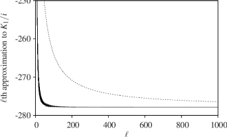
Figure 3: Convergence of the sequence on the right-hand side of (55) (dashed line) and the ‘accelerated’ sequence defined by the right-hand side of (57) (solid line). Shown are the $\ell$th approximations to the Stokes constant $K_{1}$ [the $\ell$th members of the sequences (55) and (57)] divided by $i$ to get a real value. In this plot, $\mu=0$ and $k=0.5$.

Figure 4: The Stokes constant $K_{1}$ for various values of $\mu$. Note the logarithmic scale on the vertical axis. The downward spikes extend all the way to $-\infty$; hence each spike corresponds to a zero crossing. Each panel shows only a portion of the full range $0\leq k\leq\pi/2$; there are no additional zero crossings in the part which is not shown.

Figure 4(a) shows the calculated Stokes constant as a function of $k$ for various values of the saturation parameter $\mu$. First of all, $K_{1}(k)$ does not have any zeros in the case of the cubic nonlinearity ($\mu=0$). This means that solitons of the cubic one-site discrete NLS equation [eq. (2) with $\mu=0$] cannot propagate without losing energy to radiation. For $\mu=3$ the Stokes constant does have a zero, but at a value of $k$ smaller than $k^{(1)}_{\rm max}$ (where $k^{(1)}_{\rm max}\approx 0.22=0.07\pi$). Since higher radiation modes do exist in this range of $k$, there will still be radiation from the soliton – unless the ‘higher’ Stokes constants $K_{2}(k)$, $K_{3}(k)$,…, happen to be zero at the same value of $k$. Finally, for $\mu=4$ the zero is seen to have moved just above $k^{(1)}_{\rm max}$ and for $\mu=6$ it has an even higher value. There are no $\mathcal{Q}_{2},\mathcal{Q}_{3},\ldots$ radiations for these $k$; hence the zeros of $K_{1}(k)$ define the carrier wavenumbers at which the soliton ‘slides’ – i.e. travels without emitting any radiation. Equation (17) then gives the corresponding sliding velocities, for each $\epsilon$.

Figure 4(b) shows the Stokes constant $K_{1}(k)$ for higher values of the parameter $\mu$. For $\mu=12$ a second zero of the Stokes constant has appeared while for $\mu=25$, the function $K_{1}(k)$ has three zeros. As $\mu$ is increased, the existing zeros move to larger values of $k$ while new ones emerge at the origin of the $k$ axis.

III.7 Radiation waves

For not very large $|X|$, the solution $\psi_{s}$ is close to the localised pulse found by means of the perturbation expansion in section II. As $X\to+\infty$, it tends to zero, by definition, while the $X\to-\infty$ asymptotic behaviour is found from $\psi_{s}=\psi_{u}+\Psi$. Here the solution $\psi_{u}$ decays to zero as $X\to-\infty$ and hence $\psi_{s}$ approaches the oscillatory waveform $\Psi$ given by eqs (24), (25), and (36):

$$\psi_{s}(X)\to\sum_{n}K_{n}^{*}e^{-\pi\mathcal{Q}_{n}/2\epsilon}\\ \times\left[1+\epsilon\frac{4i\cos k\tan X}{2\sin(k+\mathcal{Q}_{n})-v}+{\cal O}\left({\epsilon^{2}}\right)\right]e^{i\mathcal{Q}_{n}X/\epsilon}$$ (59)

as $X\to-\infty$. Equation (59) describes a radiation background over which the soliton is superimposed. As we have explained, we can ignore all but the first term in the sum.

To determine whether the radiation is emitted by the soliton or being fed into it from outside sources, we consider a harmonic solution $\psi=e^{i\mathcal{Q}X/\epsilon-i\Omega t}$ of the linearised eq. (21); the corresponding dispersion relation is

$$\Omega(\mathcal{Q})=-2\cos(k+\mathcal{Q})+\omega-\mathcal{Q}v.$$

The radiation background $\Psi$ consists of harmonics with $\Omega=0$ and $\mathcal{Q}=\mathcal{Q}_{n}$ where $\mathcal{Q}_{n}$ are roots of eq. (18). The group velocities of these harmonic waves are given by

$$\Omega^{\prime}(\mathcal{Q}_{n})=2\sin(k+\mathcal{Q}_{n})-v.$$ (60)

The $\mathcal{Q}_{n}$’s are zeros of the function $\Omega(\mathcal{Q})$ and the group velocities are the slopes of this function at its zeros; thus the group velocities $\Omega^{\prime}(\mathcal{Q}_{1})$, $\Omega^{\prime}(\mathcal{Q}_{2})$,…, have alternating signs. The first one, which is the only one that concerns us in this work, must be negative. Indeed, the value

$$\Omega(0)=-2\cos k+\omega=2\cos k(\cosh\epsilon-1)$$

is positive, and hence the slope of the function $\Omega(\mathcal{Q})$ as it crosses the $\mathcal{Q}$ axis at $\mathcal{Q}_{1}>0$ is negative. Therefore, the first radiation mode, extending to $-\infty$, carries energy away from the soliton.

The even-numbered radiation modes (where present) in our asymptotic solution (59) have positive group velocities and hence describe the flux of energy fed into the system at the left infinity. A more interesting situation is obviously the one with no incoming radiation; the corresponding solution is obtained by subtracting off the required multiple of the solution of the linearised equation, e.g. $e^{i\mathcal{Q}_{2}X/\epsilon}$. One would then have a pulse leaving the odd modes in its wake and sending even modes ahead of it.

If the first Stokes constant $K_{1}(k)$ has a zero at some $k=k_{1}$ while $\mathcal{Q}_{1}$ is the only radiation mode available (as happens in our saturable model with $\mu$ greater than approximately $4$), then according to eq. (59), the radiation from the soliton with the carrier-wave wavenumber $k_{1}$ is suppressed completely.

IV Time evolution of a radiating soliton

IV.1 Amplitude-wavenumber dynamical system

To find the radiation-induced evolution of the travelling soliton, we use conserved quantities of the advance-delay equation associated with eq. (2). In the reference frame moving at the soliton velocity $v$ this equation reads

$$i\varphi_{t}+\varphi(x+1,t)+\varphi(x-1,t)-iv\varphi_{x}+\frac{2|\varphi|^{2}\varphi}{1+\mu|\varphi|^{2}}=0.$$ (61)

The discrete variable $\phi_{n}(t)$ in eq. (2) is related to the value of the continuous variable $\varphi(x,t)$ at the point $x=n-vt$: $\phi_{n}(t)=\varphi(n-vt,t)$. For future use, we also mention the relation between $\varphi(x,t)$ and the corresponding solution of eq. (21):

$$\varphi(x,t)=\psi(X,t)e^{ik(x+vt)+i\omega t}.$$ (62)

We first consider the number of particles integral:

$$N=\int_{a}^{b}|\varphi|^{2}dx.$$

Multiplying eq. (61) by ${\varphi}^{\ast}$, subtracting the complex conjugate and integrating yields the rate of change of the integral $N$:

$$i\frac{dN}{dt} =\int_{a-1}^{a}(\varphi^{+}{\varphi}^{\ast}-c.c.)dx$$

$$\quad+\int_{b}^{b+1}(\varphi^{-}{\varphi}^{\ast}-c.c.)dx+iv|\varphi|^{2}\Big{|}_{a}^{b}.$$ (63)

In eq. (IV.1), $\varphi^{\pm}\equiv\varphi(x\pm 1,t)$ and $c.c.$ stands for the complex conjugate of the immediately preceding term. The integration limits $a<0$ and $b>0$ are assumed to be large ($|a|,b\gg\epsilon^{-1}$) but finite; for example one can take $a,b={\cal O}(\epsilon^{-2})$.

Consider the soliton moving with a positive velocity and leaving radiation in its wake. This configuration is described by the solution $\psi_{s}$ of eq. (21); the corresponding solution of eq. (61) has the asymptotic behaviour $\varphi_{s}\to 0$ as $x\to+\infty$. Substituting the leading-order expression (23) for the soliton’s radiation tail into eq. (62) yields the asymptotic behaviour at the other infinity:

$$\varphi_{s}(x,t)\to\sum_{n}A_{n}[1+{\cal O}\left({\epsilon}\right)]e^{i(k+{\cal Q}_{n})x+i(\omega+kv)t}$$ (64)

as $x\to-\infty$. Since, as we have explained above, the $\mathcal{Q}_{1}$ radiation is dominant, it is sufficient to keep only the $n=1$ term in (64).

Substituting (64) into (IV.1) and evaluating the integral over the region $(a-1,a)$ in the soliton’s wake, we obtain

$$\frac{dN}{dt}=|K_{1}|^{2}e^{-\pi\mathcal{Q}_{1}/\epsilon}[2\sin(k+\mathcal{Q}_{1})-v],$$ (65)

where we have used eq. (36). Note that $[2\sin(k+\mathcal{Q}_{1})-v]$ is the group velocity of the first radiation mode, $\Omega^{\prime}(\mathcal{Q}_{1})$, which, as we have established, is negative; hence ${\dot{N}}\leq 0$.

We now turn to the momentum integral,

$$P=\frac{i}{2}\int_{a}^{b}({\varphi}^{\ast}_{x}\varphi-\varphi_{x}{\varphi}^{\ast})dx.$$

Multiplying (61) by ${\varphi}^{\ast}_{x}$, adding its complex conjugate and integrating, gives the rate equation

$$\frac{dP}{dt}=\int_{a-1}^{a}(\varphi^{+}{\varphi}^{\ast}_{x}+c.c.)dx-\int_{b}^{b+1}(\varphi^{-}{\varphi}^{\ast}_{x}+c.c.)dx\\ +\frac{i}{2}(\varphi{\varphi_{t}}^{\ast}-{\varphi}^{\ast}\varphi_{t})\Big{|}_{a}^{b}-(\varphi^{+})^{*}\varphi\Big{|}_{a-1}^{b}-(\varphi^{-})^{*}\varphi\Big{|}_{a}^{b+1}\\ -\left[\frac{2}{\mu}|\varphi|^{2}-\frac{2}{\mu^{2}}\ln\left(1+\mu|\varphi|^{2}\right)\right]_{a}^{b}.$$ (66)

Evaluating the right-hand side of (66) similarly to the way we obtained (65) and substituting eq. (18) for $\omega$, produces

$$\frac{dP}{dt}=|K_{1}|^{2}e^{-\pi\mathcal{Q}_{1}/\epsilon}(k+\mathcal{Q}_{1})[2\sin(k+\mathcal{Q}_{1})-v].$$ (67)

Using the leading-order term of the perturbative solution (II.3) and eq. (62), we can express $N$ and $P$ via $\epsilon$ and $k$:

$$N=2\epsilon\cos k+{\cal O}\left({\epsilon^{2}}\right),$$

$$P=2k\epsilon\cos k+{\cal O}\left({\epsilon^{2}}\right).$$

In calculating $N$ and $P$ we had to integrate from $X=\epsilon a$ to $X=\epsilon b$. Since the integrands decay exponentially, and since $a<0$ and $b>0$ were assumed to be much larger than $\epsilon^{-1}$ in absolute value, it was legitimate to replace these limits with $-\infty$ and $\infty$, respectively. The error introduced in this way is exponentially small in $\epsilon$.

Taking time derivatives of $N$ and $P$ above and discarding $\epsilon^{1}$ corrections to $\epsilon^{0}$ terms, we deduce that

$${\dot{\epsilon}} =\frac{\dot{N}+\tan k(\dot{P}-k\dot{N})}{2\cos k},$$

$${\dot{k}} =\frac{\dot{P}-k\dot{N}}{2\epsilon\cos k}.$$

Finally, substituting for $\dot{N}$ and $\dot{P}$ from eqs (65) and (67), we arrive at the dynamical system

$$\dot{\epsilon} =|K_{1}(k)|^{2}e^{-\pi\mathcal{Q}_{1}/\epsilon}\,\Omega^{\prime}(\mathcal{Q}_{1})\,\frac{1+\mathcal{Q}_{1}\tan k}{2\cos k},$$ (68a)

$$\dot{k} =|K_{1}(k)|^{2}e^{-\pi\mathcal{Q}_{1}/\epsilon}\,\Omega^{\prime}(\mathcal{Q}_{1})\,\frac{\mathcal{Q}_{1}}{2\epsilon\cos k},$$ (68b)

where the group velocity $\Omega^{\prime}(\mathcal{Q}_{1})=2\sin(k+\mathcal{Q}_{1})-v$ with $v=2(\sinh\epsilon/\epsilon)\sin k$, and $\mathcal{Q}_{1}=\mathcal{Q}_{1}(\epsilon,k)$ is the smallest root of eq. (19).

Figure 5: The phase portrait of the system (68) in the case (a) where the Stokes constant $K_{1}(k)$ does not have zeros, and (b) where $K_{1}(k)$ has one zero. In (b), the dashed line is the line of nonisolated fixed points $k=k_{1}$. Note that in (b), the phase portrait has been replotted on the $(\epsilon,v)$ plane; hence the dashed line gives the value of the sliding velocity for each value of $\epsilon$. In (a), $\mu=0$; in (b), $\mu=6$.

IV.2 Soliton’s deceleration and sliding velocities

The vector field (68) is defined for $k\geq k^{(1)}_{\rm min}$, where $k^{(1)}_{\rm min}$ is the value of $k$ for which the roots $\mathcal{Q}_{1}$ and $\mathcal{Q}_{2}$ merge in fig. 1 (i.e. the smallest value of $k$ for which the roots $\mathcal{Q}_{1}$ and $\mathcal{Q}_{2}$ still exist). When $k=k^{(1)}_{\rm min}$, the group velocity $\Omega^{\prime}(\mathcal{Q}_{1})$ becomes equal to zero; therefore, the equation $k=k^{(1)}_{\rm min}(\epsilon)$ defines a line of (nonisolated) fixed points of the system (68). Assume, first, that the saturation parameter $\mu$ is such that $K_{1}(k)$ does not vanish for any $k$. For $k>k^{(1)}_{\rm min}$, the factor $\Omega^{\prime}(\mathcal{Q}_{1})$ in (68b) is negative; since $\mathcal{Q}_{1}$ and $\cos k$ are positive for all $0<k\leq\pi/2$, the derivative $\dot{k}$ satisfies $\dot{k}\leq 0$ for all times. Hence, all trajectories are flowing towards the line $k=k^{(1)}_{\rm min}(\epsilon)$ from above. It is worth noting that the derivative $\dot{\epsilon}$ is also negative, and that the $k$ axis is also a line of nonisolated fixed points. However, no trajectories will end there as follows from the equation

$$\frac{d\epsilon}{dk}=\epsilon\left[\tan k+\frac{1}{\mathcal{Q}_{1}(k,\epsilon)}\right],$$

which is a consequence of (68a) and (68b).

Representative trajectories are plotted in fig. 5(a). Since $k^{(1)}_{\rm min}(\epsilon)\approx\epsilon^{2}/4\pi$ is very small for small $\epsilon$, the line $k=k^{(1)}_{\rm min}(\epsilon)$ is practically indistinguishable from the horizontal axis. Therefore, we can assert that, to a good accuracy, $k\to 0$ as $t\to\infty$. This means that the soliton stops moving – and stops decaying at the same time.

For $k$ smaller than $k^{(1)}_{\rm min}$, the vector field (68) is undefined and we cannot use it to find out what happens to the soliton after $k$ has reached $k^{(1)}_{\rm min}$. The reason for this is that the soliton stops radiating at the wavenumber $\mathcal{Q}_{1}$ as $k$ drops below $k^{(1)}_{\rm min}$. In fact our analysis becomes invalid as soon as $k$ becomes $\mathcal{O}(\epsilon^{2})$—i.e. even before $k$ reaches $k^{(1)}_{\rm min}$—because we can no longer disregard the $n=2$ radiation here. At the qualitative level it is obvious, however, that the parameter $k$ should continue to decay all the way to zero, in a cascade way. First, the $n=2$ radiation will become as intense as the $n=1$ mode when $k$ approaches $\epsilon^{2}/4\pi$. Subsequently—i.e. for $k$ smaller than $\epsilon^{2}/4\pi$—the $n=3$ harmonic will replace the radiation with the wavenumbers $\mathcal{Q}_{1}$ and $\mathcal{Q}_{2}$ as a dominant mode. The $n=4$ mode will become equally intense near $k=k^{(2)}_{\rm min}\approx\epsilon^{2}/8\pi$; as $k$ drops below $\epsilon^{2}/8\pi$, both $\mathcal{Q}_{3}$ and $\mathcal{Q}_{4}$ will cede to $\mathcal{Q}_{5}$, and so on.

If $\mu$ is such that the Stokes constant $K_{1}(k)$ vanishes at one or more values of $k$, the system has one or more lines of nonisolated fixed points, $k=k_{i}$. The corresponding values of $v$, $v=v_{i}(\epsilon)\equiv 2(\sinh\epsilon/\epsilon)\sin k_{i}$, define the sliding velocities of the soliton – i.e. velocities at which the soliton moves without radiative friction. One such velocity is shown by the dashed line in fig. 5(b). The fixed points $(\epsilon,k_{i})$ are semistable; for $k$ above $k_{i}$, the flow is towards the line $k=k_{i}$ but when $k$ is below $k_{i}$, the flow is directed away from this straight line [see fig. 5(b)]. Since both $\dot{\epsilon}$ and $\dot{k}$ are negative, the soliton’s velocity $v=2(\sinh\epsilon/\epsilon)\sin k$ will generally be decreasing – until it hits the nearest underlying sliding velocity $v_{i}$ and locks on to it. The ensuing sliding motion will be unstable; a small perturbation will be sufficient to take the soliton out of the sliding regime after which it will resume its radiative deceleration. However, since $\dot{k}$ is proportional to the square of the Stokes constant and not to $K_{1}(k)$ itself, small perturbations $\delta k$ will be growing linearly, not exponentially, in $t$. As a result, the soliton may spend a fairly long time sliding at the velocity $v_{i}$. It is therefore not unreasonable to classify this sliding motion as metastable.

We conclude that the soliton becomes pinned (i.e. $k\rightarrow 0$ and so $v\to 0$) before it has decayed fully (i.e. before the amplitude $\epsilon$ has decreased to zero). The exponential dependence of $\dot{\epsilon}$ and $\dot{k}$ on $1/\epsilon$ implies that tall, narrow pulses will be pinned very quickly while short, broad ones will travel for a very long time before they have slowed appreciably. Next, if $\mu$ is such that there is one or more sliding velocity available in the system, and if the soliton is initially moving faster than some of these, its deceleration will be interrupted by long periods of undamped motion at the corresponding sliding velocities.

Figure 6: The soliton’s decay rate as a function of its velocity, for fixed $\epsilon=0.1$. (Here $\mu=0$.) In the inset, the same curve is replotted using a logarithmic scale on the vertical axis.

It is worth reemphasising here that if the amplitude $\epsilon$ is small, then even if the soliton is not sliding, its deceleration will be so slow that it will spend an exponentially long time travelling with virtually unchanged amplitude and speed. The deceleration rate $-{\dot{v}}/v$ is shown in fig. 6, as a function of the soliton’s velocity $v$, for fixed amplitude $\epsilon$. Note that the decay rate drops, exponentially, as the velocity is decreased; this drop is due to the exponential factor $e^{-\pi\mathcal{Q}_{1}/\epsilon}$ in eq. (68). As the velocity $v$ (and hence the wavenumber $k$) decreases, the root $\mathcal{Q}_{1}(\epsilon,k)$ grows towards the limit value of approximately $2\pi$ (see fig. 1). This variation in $\mathcal{Q}_{1}$ is amplified by the division by small $\epsilon$ and exponentiation in $e^{-\pi\mathcal{Q}_{1}/\epsilon}$.

V Concluding remarks

V.1 Summary

In this paper, we have constructed the moving discrete soliton of the saturable NLS equation (2) [and hence (1)] as an asymptotic expansion in powers of its amplitude. The saturable nonlinearity includes the cubic NLS as a particular case (for which $\mu=0$). Our perturbation procedure is a variant of the Lindstedt–Poincaré technique where corrections to the parameters of the solution are calculated along with the calculation of the solution itself. Although the resulting asymptotic series (II.3) for the soliton is generally not convergent, the associated expansions for its frequency and velocity sum up to exact explicit expressions (17).

From the divergence of the asymptotic series (II.3) it follows, in particular, that the travelling discrete soliton does not decay to zero at least at one of the two infinities. Instead, the soliton approaches, as $X\to\infty$ or $X\to-\infty$, an oscillatory resonant background (23) where the amplitudes $A_{n}$ of its constituent harmonic waves lie beyond all orders of $\epsilon$. For the soliton moving with a positive velocity and approaching zero as $X\to\infty$, the oscillatory background at the left infinity represents the Cherenkov radiation left in the soliton’s wake. To evaluate the amplitudes of the harmonic waves arising as $X\to-\infty$, we have continued the radiating soliton into the complex plane, where it exhibits singularities. We then matched the asymptotic expansion (34) of the background near the lowest singularity on the imaginary $X$ axis to the far-field asymptotic expansion (31) of the background solution of the ‘inner’ equation – i.e. of the advance-delay equation ‘zoomed in’ on this singularity. The asymptotic expansions here are in inverse powers of the zoomed variable, $y$. The amplitudes of the radiation waves were found to be exponentially small in $\epsilon$, with the pre-exponential factors (the so-called Stokes constants) being dependent only on the soliton’s carrier-wave wavenumber. Representing solutions to the inner equation as Borel sums of their asymptotic expansions, the Stokes constants can be related to the expansion coefficients; we have calculated these coefficients numerically, using algebraic recurrence relations.

The upshot of the calculation of the leading Stokes constant $K_{1}$ is that in the case of the cubic nonlinearity (i.e. for $\mu=0$), $K_{1}(k)$ does not vanish for any $k$. This means that the cubic discrete soliton cannot ‘slide’ – i.e. cannot move without radiative friction. The saturable solitons, on the other hand, can slide provided the saturation parameter $\mu$ is large enough. This is because, for a sufficiently large $\mu$, the Stokes constant $K_{1}(k)$ is found to have one or more zeros $k_{1},k_{2},\ldots$. Since the soliton with wavenumber $k>0.22$ can have no higher-order resonances, those zeros which satisfy $k_{i}>0.22$ do define the wavenumbers at which sliding motion occurs. For each value of the soliton’s amplitude $\epsilon$, the formula (17) then gives the sliding velocities $v(k_{i},\epsilon)$.

The calculation of asymptotics beyond all orders is useful not only for determining the sliding velocities. Knowing the radiation amplitudes has allowed us to derive a two-dimensional dynamical system (68) for the soliton’s parameters. Trajectories of this dynamical system describe the evolution of the soliton travelling at a generic speed. The evolution turns out to be simple: If $\mu$ is such that the Stokes constant $K_{1}(k)$ does not vanish anywhere in the region $k>0.22$, the soliton decelerates, although very slowly. Eventually it becomes pinned to the lattice with a decreased but finite amplitude. However, if $\mu$ is such that there are sliding velocities in the system, and if the soliton starts its motion with the velocity higher than some of these then, although it will finally become pinned to the lattice, its deceleration will be interrupted by long periods of metastable sliding motion at these isolated velocities.

V.2 Concluding remarks

It is interesting to tie up the above results with our previous work on exceptional discretisations of the $\phi^{4}$ model OPB . In that case we discovered that for some exceptional models (in which the stationary soliton possesses an effective translational symmetry), sliding velocities, at which the radiation disappears, do exist. The fact that all these models involve a complicated nonlocal discretisation of the nonlinearity leads one to wonder whether the nonlinearity has to be discretised nonlocally in order for sliding solitons to exist. This question is answered—negatively—by our present work which gives a counterexample of a simple, local and physically motivated nonlinearity supporting sliding solitons.

A remaining open issue is whether exceptionality of the system is a prerequisite for the existence of sliding solitary waves. Indeed, we have yet to encounter a nonexceptional discrete system permitting sliding motion.

We conclude this section by placing our results in the context of earlier studies of discrete solitons.

Moving solitons in the cubic DNLS equation have previously been studied by Ablowitz, Musslimani, and Biondini ablowitz (among others), using a numerical technique based on discrete Fourier transforms as well as perturbation expansions for small velocities. As we have done, these authors suggest that sliding (radiationless) solitons may not exist. They also observe, with the aid of numerical simulations, that strongly localised pulses are pinned quickly to the lattice, while broader ones are more mobile – results which are in agreement with ours.

Duncan, Eilbeck, Feddersen and Wattis Feddersen ; duncan have studied the bifurcation of periodic travelling waves from constant solutions in the cubic DNLS equation, using numerical path-following techniques. They find that the paths terminate when the soliton’s amplitude reaches a certain limit value, and in the light of our results it seems likely that this is the point at which the radiation becomes large enough to have an effect on the numerics.

Solitary waves which decay to constant values at the spatial infinities, despite the fact that the generic asymptotic behaviour in the underlying model is oscillatory, are commonly referred to as embedded solitons. An example is given by the sliding solitons reported in this paper as well as the sliding kinks of OPB ; both types of solitary waves propagate without exciting the resonant background oscillations. Embedded solitons have been studied for some time in continuous systems embedded_review , but their history in lattice equations is younger. Recently, Malomed, González-Pérez-Sandi, Fujioka, Espinosa-Cerón and Rodríguez have considered certain lattice equations with next-to-nearest-neighbour couplings and shown (by means of explicit solutions) that both stationary Malomed_embedded_0 and moving Malomed_embedded embedded solitons exist. Stationary embedded solitons in discrete waveguide arrays have also been analysed by Yagasaki, Champneys and Malomed Malomed_embedded_2 .

Finally, while preparing the revised version of this paper, we learnt that Melvin, Champneys, Kevrekidis, and Cuevas have obtained results very similar to ours. Using a combination of intuitive arguments and numerical computations, they have found sliding solitons for certain values of the parameters of a saturable DNLS model melvin .

Appendix A Convolution theorem for the Laplace transform in the complex plane

This appendix deals with the convolution property of the modified Laplace transform of the form (37), where the integration is along an infinite contour in the complex plane rather than the positive real axis. In the context of asymptotics beyond all orders, this transform was pioneered by Grimshaw and Joshi GrimshawJoshi . Since no proof of the convolution result (39) is available in literature, and since it requires a nontrivial property (concavity) of the integration contour, we produce such a proof here.

We wish to show that

$$\int_{\gamma}e^{-pz}F(p)dp\int_{\gamma}e^{-p^{\prime}z}G(p^{\prime})dp^{\prime}$$

$$= \int_{\gamma}e^{-pz}\left[\int_{0}^{p}F(p_{1})G(p-p_{1})dp_{1}\right]dp,$$ (69)

where $\int_{0}^{p}$ stands for an integral along the curve $\gamma$ from the origin to the point $p$ on that curve. We assume that the curve $\gamma$ extends from the origin to infinity on the complex plane; lies in its first quadrant ($\operatorname{Re}p>0$, $\operatorname{Im}p>0$); is described as a graph of a single-valued function $\operatorname{Im}p=f(\operatorname{Re}p)$ (i.e. never turns back on itself), and is concave-up everywhere:

$$\frac{d^{2}f}{d(\operatorname{Re}p)^{2}}>0\quad\text{for}\ p\ \text{on}\,\gamma.$$

We also assume that the function $G(p)$ is analytic in the region between the contour $\gamma$ and the imaginary axis.

Figure 7: Deformation of the integration contour $\Gamma_{p}$ to $\Gamma_{p}^{\prime}$.

We begin by writing the left-hand side of (A) as

$$\int_{\gamma}\int_{\gamma}e^{-(p+p^{\prime})z}F(p)G(p^{\prime})dp^{\prime}dp$$

$$= \int_{\gamma}F(p)\left[\int_{\Gamma_{p}}e^{-rz}G(r-p)dr\right]dp,$$ (70)

where $r=p^{\prime}+p$. The curve $\Gamma_{p}$ is the path traced out by $r$ as $p^{\prime}$ traces out the curve $\gamma$, for a given $p$ (which also lies on $\gamma$) – this is depicted in fig. 7. The path $\Gamma_{p}$ is the same as the path $\gamma$ but translated from the origin to the point $p$.

For each given $p$ we deform the path $\Gamma_{p}$ so that it now lies on $\gamma$, still starting at the point $p$. We call this deformed path $\Gamma_{p}^{\prime}$. The point $r-p=p^{\prime}$, which lay on the path $\gamma$ before the deformation, will now move inside the region bounded by $\gamma$ (i.e. the region to the left of $\gamma$), since all points on $\Gamma_{p}^{\prime}$ lie inside the region bounded by $\Gamma_{p}$. This follows from the fact that the path $\Gamma_{p}$ is concave-up. The point $r-p$ will, however, stay to the right of the imaginary axis, since after the deformation all points $r$ on $\Gamma_{p}^{\prime}$ lie to the right of the point $p$. This follows from the fact that the curve $\gamma$ never turns back on itself. Since $G(p^{\prime})$ is analytic for all $p^{\prime}$ between the imaginary axis and $\gamma$, the value of the integral (70) will not be affected by the deformation. [In the particular case of the functions $U(p)$ and $W(p)$ considered in section III.5, we have deliberately chosen the contours of integration so that the analyticity condition is satisfied.]

After the deformation, both integrals in (70) follow the path $\gamma$, with the inner one starting at the point $p$. By parameterising the path $\gamma$ it is now straightforward to change the order of integration, and end up with the desired result (A).

The argument holds, with the obvious modifications, for paths in the second quadrant.

Appendix B Proof that singularities do not accumulate to the imaginary axis

The roots of eq. (40) with the top and bottom signs give singularities of $U(p)$ and $W(p)$, respectively. Our aim here is to show that the integration contours $\gamma_{u}$ and $\gamma_{s}$ in section III.5 can be chosen to lie above all the complex singularities – i.e., that singularities of $U(p)$ and $W(p)$ do not accumulate to the imaginary axis.

The roots of eq. (40) are zeros of the functions $F(\pm p)$, where

$$F(p)\equiv\cosh p-1-i\tan k(\sinh p-p).$$ (71)

The imaginary zeros of $F(p)$ are at $p=-iq_{n}$, where $q_{n}$ are the real roots of eq. (30). We let $N$ denote the number of these imaginary zeros; for $k\neq 0$, $N$ is finite. We recall that all $q_{n}$ are positive; hence all $N$ imaginary zeros of $F(p)$ are on the negative imaginary axis, and all $N$ zeros of $F(-p)$ on the positive imaginary axis.

Let $\kappa$ and $q$ be the real and imaginary part of $p$: $p=\kappa+iq$. We let $\mathcal{D}$ denote the rectangular region in the complex-$p$ plane bounded by the vertical lines $\kappa=\pm\varepsilon$ and horizontal lines $q=\varepsilon^{1/2}$ and $q=Q$, where $\varepsilon$ is small and $Q$ is large enough for the region to contain all $N$ zeros of $F(-p)$ on the positive imaginary axis. By the argument principle, the total number of (complex) zeros of the function $F(-p)$ in the region $\mathcal{D}$ is given by $(2\pi)^{-1}$ times the variation of its argument (i.e., its phase) along the boundary of $\mathcal{D}$. In a similar way, one may count the number of zeros of the function $F(p)$ in $\mathcal{D}$.

We have

$$\tan\arg F(\pm p)\!=\!\frac{\sinh\kappa\sin q\mp\tan k(\sinh\kappa\cos q-\kappa)}{\cosh\kappa\cos q-1\pm\tan k(\cosh\kappa\sin q-q)}.$$

Points on the vertical line $\kappa=\varepsilon$ satisfy

$$\tan\arg F(\pm p)\approx{-\varepsilon}\frac{d}{dq}\ln|1-\cos q\pm\tan k(q-\sin q)|.$$ (72)

Consider, first, the case of the bottom sign in eq. (72). The expression between the bars in (72) crosses through zero $N$ times as the line $\kappa=\varepsilon$ is traced out. Each time zero is crossed, the logarithmic derivative in (72) jumps from $-\infty$ to $+\infty$, and the argument of $F(-p)$ increases by $\pi$ as we move from one crossing to the next one. The net increase of the argument as the line $\kappa=\varepsilon$ is traversed from its bottom to the top, is $N\pi$. In the case of the top sign in (72), on the other hand, the expression in $|\ldots|$ never crosses through zero and hence the total increment of the argument of $F(p)$ is zero.

As we move along the vertical line $\kappa=-\varepsilon$ from top to bottom, the argument of $F(-p)$ increases by another $N\pi$ while the argument of $F(p)$ does not acquire any increment. Since there are no zero crossings on the horizontal segments, the net change of the argument of $F(-p)$ along the boundary of $\mathcal{D}$ is $2N\pi$ while the total increment of ${\rm arg\/}\,F(p)$ is zero. Therefore $F(-p)$ has only $N$ zeros in the region $\mathcal{D}$ (and they all lie on the imaginary axis) while the function $F(p)$ has no zeros in $\mathcal{D}$. This implies that complex singularities of $U(p)$ and $W(p)$ cannot accumulate to the positive imaginary axis.

References

- (1) O. Braun and Yu. S. Kivshar, Phys. Rep. 306, 1 (1998).
- (2) D. Hennig and G. P. Tsironis Phys. Rep. 307, 333 (1999).
- (3) A. Scott, Nonlinear Science: emergence and dynamics of coherent structures (Oxford University Press, 1999).
- (4) D. N. Christodoulides, F. Lederer, and Y. Silberberg, Nature 424, 817 (2003).
- (5) D. K. Campbell, S. Flach, and Yu. S. Kivshar, Phys. Today 57(1), 43 (2004).
- (6) A. Trombettoni and A. Smerzi, Phys. Rev. Lett. 86, 2353 (2001).
- (7) H. Feddersen, in Nonlinear Coherent Structures in Physics and Biology. Proceedings of the 7th Interdisciplinary Workshop Held at Dijon, France, 4-6 June 1991. Eds. M. Remoissenet and M. Peyrard, Lecture Notes in Physics vol. 393 (Springer, Berlin, 1991), pp. 159–167.
- (8) D. B. Duncan, J. C. Eilbeck, H. Feddersen, and J. A. D. Wattis, Physica D 68, 1 (1993).
- (9) S. Flach and C. R. Willis, Phys. Rep. 295, 181 (1998).
- (10) S. Flach and K. Kladko, Physica D 127, 61 (1999).
- (11) S. Flach, Y. Zolotaryuk and K. Kladko, Phys. Rev. E 59, 6105 (1999).
- (12) P. G. Kevrekidis, K. Ø. Rasmussen, and A. R. Bishop, Int. J. Mod. Phys. B 15, 2833 (2001).
- (13) M. J. Ablowitz, Z. H. Musslimani, and G. Biondini, Phys. Rev. E 65, 026602 (2002).
- (14) K. Kundu, J. Phys. A: Math. Gen. 35, 8109 (2002).
- (15) J. C. Eilbeck and M. Johansson, in Proceedings of the Third Conference on Localization and Energy Transfer in Nonlinear Systems, San Lorenzo de El Escorial, Madrid, Spain, June 17–21, 2002 (World Scientific, Singapore, 2003), pp. 44–67.
- (16) I. E. Papacharalampous, P. G. Kevrekidis, B. A. Malomed, and D. J. Frantzeskakis, Phys. Rev. E 68, 046604 (2003).
- (17) S. V. Dmitriev, P. G. Kevrekidis, B. A. Malomed, and D. J. Frantzeskakis, Phys. Rev. E 68, 056603 (2003).
- (18) D. E. Pelinovsky and V. M. Rothos, Physica D 202, 16 (2005).
- (19) J. Cuevas, B. A. Malomed, and P. G. Kevrekidis, Phys. Rev. E 71, 066614 (2005).
- (20) J. Gómez-Gardeñez, F. Falo, and L. M. Floría, Phys. Lett. A 332, 213 (2004).
- (21) J. Gómez-Gardeñez, L. M. Floría, M. Peyrard, and A. R. Bishop, Chaos 14, 1130 (2004).
- (22) N. K. Efremidis, S. Sears, D. N. Christodoulides, J. W. Fleischer, and M. Segev, Phys. Rev. E 66, 046602 (2002).
- (23) J. W. Fleischer, T. Carmon, M. Segev, N. K. Efremidis, and D. N. Christodoulides, Phys. Rev. Lett. 90, 023902 (2003).
- (24) F. Chen, C. E. Rüter, D. Runde, D. Kip, V. Shandarov, O. Manela, and M. Segev, Opt. Exp. 13, 4314 (2005).
- (25) J. W. Fleischer, M. Segev, N. K. Efremidis, and D. N. Christodoulides, Nature 422, 147 (2003).
- (26) L. Hadžievski, A. Maluckov, M. Stepić, and D. Kip, Phys. Rev. Lett. 93, 033901 (2004).
- (27) M. Stepić, D. Kip, L. Hadžievski, and A. Maluckov, Phys. Rev. E 69, 066618 (2004).
- (28) J. Cuevas and J. C. Eilbeck, Phys. Lett. A 358, 15 (2006).
- (29) R. A. Vicencio and M. Johansson, Phys. Rev. E 73, 046602 (2006).
- (30) S. Gatz and J. Herrmann, J. Opt. Soc. Am. B 8, 2296 (1991).
- (31) S. Gatz and J. Herrmann, Opt. Lett. 17, 484 (1992).
- (32) V. Tikhonenko, J. Christou, and B. Luther-Davies, Phys. Rev. Lett. 76, 2698 (1996).
- (33) F. Vidal and T. W. Johnston, Phys. Rev. E 55, 3571 (1997).
- (34) A. Khare, K. Ø. Rasmussen, M. R. Samuelsen, and A. Saxena, J. Phys. A: Math. Gen. 38, 807 (2005).
- (35) I. V. Barashenkov, O. F. Oxtoby, and D. E. Pelinovsky, Phys. Rev. E 72 035602(R) (2005).
- (36) O. F. Oxtoby, D. E. Pelinovsky, and I. V. Barashenkov, Nonlinearity 19, 217 (2006).
- (37) V. O. Vinetskii and N. V. Kukhtarev, Sov. Phys. Solid State 16, 2414 (1975).
- (38) See e.g. A. H. Nayfeh and D. T. Mook, Nonlinear Oscillations (J. Wiley, New York, 1979); D. W. Jordan and P. Smith, Nonlinear Ordinary Differential Equations (Oxford University Press, 1999).
- (39) M.J. Ablowitz and J.F. Ladik, Stud. Appl. Math. 55 213 (1976); J. Math. Phys. 17 10011 (1976).
- (40) E. W. Laedke, O. Kluth, and K. H. Spatschek, Phys. Rev. E 54 4299 (1996).
- (41) D. E. Pelinovsky, Nonlinearity 19, 2695 (2006).
- (42) V. M. Eleonksii, N. E. Kulagin, N. S. Novozhilova, and V. P. Silin, Teor. Mat. Fiz. 60, 395 (1984).
- (43) H. Segur and M. D. Kruskal, Phys. Rev. Lett. 58, 747 (1987).
- (44) M. D. Kruskal and H. Segur, Stud. Appl. Math. 85, 129 (1991).
- (45) Y. Pomeau, A. Ramani, and B. Grammaticos, Physica D 31, 127 (1988).
- (46) R. H. J. Grimshaw and N. Joshi, SIAM J. Appl. Math. 55, 124 (1995).
- (47) R. H. J. Grimshaw, Stud. Appl. Math. 94, 257 (1995).
- (48) A. Tovbis, M. Tsuchiya, and C. Jaffé, Chaos 8, 665 (1998).
- (49) A. Tovbis, Contemporary Mathematics 255, 199 (2000).
- (50) A. Tovbis, Stud. Appl. Math. 104, 353 (2000).
- (51) A. Tovbis and D. Pelinovsky, Nonlinearity 19, 2277 (2006).
- (52) J. Fujioka, A. Espinosa-Cerón, and R. F. Rodríguez, Rev. Mex. Fís. 52, 6 (2006).
- (53) S. González-Pérez-Sandi, J. Fujioka, and B. A. Malomed, Physica D 197, 86 (2004).
- (54) B. A. Malomed, J. Fujioka, A. Espinosa-Cerón, R. F. Rodríguez, and S. González, Chaos 16, 013112 (2006).
- (55) K. Yagasaki, A. R. Champneys, and B. A. Malomed, Nonlinearity 18, 2591 (2005).
- (56) T. R. O. Melvin, A. R. Champneys, P. G. Kevrekidis, and J. Cuevas, Phys. Rev. Lett. 97, 124101 (2006).