Single particle Lagrangian dispersion in Bolgiano turbulence

Abstract

Single-particle dispersion in the Bolgiano–Obukhov regime of two-dimensional turbulent convection is investigated. Unlike dispersion in a flow displaying the classical K41 phenomenology, here, the leading contribution to the Lagrangian velocity fluctuations is given by the largest eddies. This implies a linear behavior in time for a typical velocity fluctuation in the time interval $t$. The contribution to the Lagrangian velocity fluctuations of local eddies (i.e. with a characteristic time of order $t$), whose space/time scalings are ruled by the Bolgiano–Obukhov theory, is thus not detectable by standard Lagrangian statistical observables. To disentangle contributions arising from the large eddies from those of local eddies, a strategy based on exit-time statistics has successfully been exploited. Lagrangian velocity increments in Bolgiano convection thus provide a physically relevant example of signal with more than smooth fluctuations.

Understanding the statistical properties of particle tracers advected by turbulent flows is a fundamental problem in turbulent research and a key ingredient for the development of stochastic models of Lagrangian dispersion P94 ; S01 ; Y02 . In the recent years there has been great improvements in theoretical FGV01 , experimental LVCAB01 ; MMMP01 ; OM00 and numerical Y01 ; BBCLT05 understanding of Lagrangian turbulence. Most of the studies have been concentrated on the so-called single particle dispersion in which the statistical objects are the Lagrangian velocity differences following a single trajectory $\delta{\bm{v}}(t)={\bm{v}}(t)-{\bm{v}}(0)$. For this quantity, dimensional analysis in statistical stationary, homogeneous and isotropic turbulence, predicts $\langle\delta v^{2}\rangle\simeq\varepsilon t$ (where $\varepsilon$ is the mean energy dissipation). The remarkable coincidence with diffusive behavior is at the basis of stochastic models of turbulent dispersion.

In this Letter we investigate on the basis of Direct Numerical Simulations (DNS) the statistics of single particle dispersion in two-dimensional Boussinesq convective turbulence. This system is characterized by an inverse cascade with scaling exponent in agreement with the Bolgiano-Obukhov theory of turbulent convection S94 . As a consequence, we expect a non-diffusive behavior for Lagrangian velocity variance. We show that a careful statistical analysis, based on exit time statistics, is necessary in order to observe the expected scaling.

The two-dimensional Boussinesq turbulent convection is described by the following set of partial differential equations CMV01 :

$$\partial_{t}\omega+{\bm{v}}\cdot{\bm{\nabla}}\omega = +\nu\Delta\omega-\beta{\bm{\nabla}}T\times{\bm{g}}$$

$$\partial_{t}T+{\bm{v}}\cdot{\bm{\nabla}}T = \kappa\Delta T$$ (1)

where $T$ is the temperature field and $\omega={\bm{\nabla}}\times{\bm{v}}$ is the scalar vorticity, ${\bm{g}}$ is the gravitational acceleration, $\beta$ is the thermal expansion coefficient and $\kappa$ and $\nu$ are molecular diffusivity and viscosity. Energy in (1) is injected by maintaining a mean temperature profile $\langle T({\bm{r}},t)\rangle={\bm{G}}\cdot{\bm{r}}$, with a constant gradient ${\bm{G}}$ pointing in the direction of gravity.

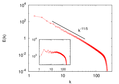
Figure 1: Energy spectrum from a Direct Numerical Simulations of Boussinesq equations at resolution $N=1024^{2}$ in stationary conditions. The line represents the dimensional prediction $E(k)\simeq k^{-11/5}$. The inset shows the spectrum compensated with the prediction.

In equation (1) the temperature field affects the vorticity through the buoyancy force, thus providing an example of active tracers. At large enough values of $\beta$, the buoyancy force can equilibrate the inertial terms in the velocity dynamics, thus providing the mechanism at the basis of the Bolgiano-Obukhov theory of turbulent convection.

Let us briefly recall the phenomenology of two-dimensional turbulent convection. The balance of buoyancy and inertial terms in equation (1) introduces the Bolgiano length scale $l_{\rm B}$ MY . At small scales, $r\ll l_{\rm B}$, the inertial term is larger than buoyancy force and the temperature is basically a passive scalar. At scales $r\gg l_{\rm B}$, buoyancy dominates and thus affects the velocity field in the inverse energy cascade. At variance with Navier-Stokes turbulence, kinetic energy is here injected at all scales in the inverse cascade. The energy flux at scale $r$ is obtained by a dimensional argument as:

$$\varepsilon_{r}=\beta{\bm{g}}\cdot\langle{\bm{v}}({\bm{x}}+{\bm{r}},t)T({\bm{x}},t)\rangle\sim r^{4/5}$$ (2)

which gives the dimensional prediction for the velocity structure functions:

$$S_{p}(r)=\langle\left(\delta_{r}v\right)^{p}\rangle\sim\left(\epsilon_{r}r\right)^{p/3}\sim r^{\zeta_{p}}$$ (3)

with $\zeta_{p}=3p/5$. The exponent of the second-order structure function ($\zeta_{2}=6/5$) gives the scaling exponent for the energy spectrum $E(k)\simeq k^{-11/5}$ which is shown in Fig. 1. It is worth remarking that detailed numerical simulations have shown that velocity fluctuations display self-similar statistics without intermittency corrections CMV01 .

The dimensional prediction for the statistics of Lagrangian velocity increments $\delta_{t}v=v(t)-v(0)$ is the following. Considering the velocity $v$ as the superposition of the contributions from eddies of different sizes, the variation $\delta_{t}v$ over a time $t$ will be given by the superposition of the variations associated to the eddies. The eddies at scale $r$, with a characteristic time $\tau_{r}\ll t$ will be decorrelated and thus give no contribution. The eddies for which $\tau_{r}\simeq t$ are the first ones to be considered. Assuming a scaling exponent $h$ for the velocity the characteristic turnover time time is $\tau_{r}\simeq\tau_{L}(r/L)^{1-h}$ ($\tau_{L}$ being characteristic time of eddies at the large scale $L$) and thus the scale of the eddies which decorrelates in a time $t$ is given by $r\simeq L(t/\tau_{L})^{1/(1-h)}$. Their contribution to the Lagrangian velocity fluctuation is thus estimated as

$$\delta_{t}v\simeq v_{L}(r/L)^{h}\simeq v_{L}(t/\tau_{L})^{q}$$ (4)

where $v_{L}$ represents velocity fluctuations at large scales and $q\equiv h/(1-h)$.

On top of this, the eddies at the large scales of the order of $L$ have to be considered. At these scales $t\ll\tau_{L}$ and the contribution to velocity fluctuations is differentiable, i.e. $\delta_{t}v\simeq(\partial_{t}v_{L})t$. The typical velocity fluctuation on the time interval $t$ is then given by the superposition of two contributions:

$$\delta_{t}v\simeq\tau_{L}(\partial_{t}v_{L})(t/\tau_{L})+v_{L}(t/\tau_{L})^{q}.$$ (5)

At small $t/\tau_{L}$ the dominant term will be the one with minimum exponent: $\delta v\sim\min(1,q)$. In the framework of the classical K41 theory ($h=1/3$, $q=1/2$) the dominant contribution in (5) is the local one which leads to the diffusive behavior $\delta_{t}v\sim t^{1/2}$. In the present case of Bolgiano convection we have $q=3/2$ and thus velocity increments in the inertial range are dominated by the infrared term $\propto t$. Therefore, a standard analysis of velocity fluctuations, i.e. Lagrangian structure functions $S^{L}_{p}(t)=\langle\left(\delta_{t}v\right)^{p}\rangle$, is unable to disentangle the Bolgiano-Obukhov scaling in the Lagrangian statistics (see Fig. 2).

Lagrangian velocity increments in Bolgiano convection provide a physically relevant example of signal with more than smooth fluctuations. The statistical analysis of this kind of signal has been recently addressed on the basis of an exit-time statistics BCLVV01 . In the following we will discuss the application of this approach to the present case and the resulting bifractal distribution of scaling exponents.

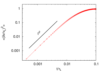
Figure 2: Second order Lagrangian structure function. The dominant ballistic regime ($\delta_{t}v\simeq t$) is evident.

The exit-time statistics is based on the time increments $T(\delta v)$ needed for a tracer to observe a change of $\delta v$ is its velocity abccv97 . Given the set of thresholds $\delta v_{n}=\rho^{n}\delta v(0)$ (with $\rho>1$), one computes the exit-times $T_{n}$ corresponding to each threshold following the tracer trajectories. Now, let us assume to have a signal $\delta v$ composed by two contributions as in (5). In the limit of small $\delta v$, the differentiable part $\propto t$ will dominate except when the derivative $\partial_{t}v_{L}$ vanishes and the local part thus becomes the leading one. For a signal with $1\leq q\leq 2$, its first derivative is a one-dimensional self-affine signal with Hölder exponent $\xi=q-1$, which thus vanishes on a fractal set of dimension $D=1-\xi=2-q$. Therefore, the probability to observe the component $O(t^{q})$ is equal to the probability to pick a point on the fractal set of dimension $D$, i.e.:

$$P(T\sim\delta v^{1/q})\sim T^{1-D}\sim(\delta v)^{1-1/q}\;.$$ (6)

By using this probability for computing the average $p$-order moments of exit-time statistics one obtains the following bi-fractal prediction BCLVV01

$$\langle T^{p}(\delta v)\rangle\sim\delta v^{\chi(p)}\;,\;\;\mbox{with}\;\;\chi(p)=\min(p,\frac{p}{q}+1-\frac{1}{q})\;.$$ (7)

According to prediction (7), low-order moments ($p\leq 1$) of the inverse statistics only see the differentiable part of the signal, while high-order moments ($p\geq 1$) are dominated by the local fluctuations $O(t^{q})$.

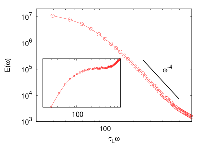
Figure 3: The spectrum $E(\omega)$ of the Lagrangian velocity increments $\delta v$. The line represent the prediction $\omega^{-4}$. The inset shows the compensated plot $E(\omega)/\omega^{-4}$. The $\omega^{-4}$ contribution is due to the superimposed more than smooth fluctuations, while the tail of the spectrum are dominated by the contributions due to the non-periodicity of the signal.

We now turn to the numerical procedure. The turbulent velocity field is obtained by direct integration of convective Navier–Stokes equation (1) with a standard, fully-dealiased pseudospectral method in a doubly periodic square domain of resolution $1024^{2}$. For numerical convenience, the viscous term in (1) has been replaced in our simulations by a hyperviscous term of order eight. Time evolution is implemented by a standard second-order Runge–Kutta scheme. Equations are integrated for about one hundred of large-scale eddy turnover times to reach a stationary state. Lagrangian trajectories are then obtained by integrating ${\bf\dot{x}}(t)={\bm{v}}({\bm{x}}(t),t)$ with the velocity at particle position obtained by linear interpolation from the nearest grid points. A single run follows 64000 particles, homogeneously distributed on the integration domain. Velocity variations $\delta_{t}v$ and exit times $T(\delta v)$ of single particles are recorded for times comparable to the integral scale. Average is performed over about 150 runs.

In Fig. 2 we show the variance of Lagrangian velocity fluctuations as a function of time. The smooth behavior $\langle(\delta_{t}v)^{2}\rangle\sim t^{2}$ is clearly observable making impossible the observation of the Bolgiano-Obukhov scaling. We remark that the same result is expected for any system with large scale domination over the local contribution, i.e. for any $q\leq 1$. Therefore, for these systems (with $h\leq 1/2$) the direct computation of Lagrangian structure functions (3) is unable to disentangle the turbulent components in the velocity field.

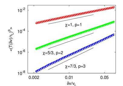
Figure 4: Exit times $\langle T^{p}(\delta v)\rangle$ of of order $p=1,2,3$ vs $\delta v$. Lines represent the predicted power-law behavior (7) with exponents $\chi(p)$.

A first check of Bolgiano scaling in Lagrangian statistics is obtained by computing the temporal energy spectrum $E(\omega)$. We remind that for an infinitely differentiable signal, the smooth contribution gives an exponential spectrum, while the $\delta_{t}v\sim t^{3/2}$ contribution gives a spectrum proportional to $\omega^{-4}$. Figure 3 clearly shows the expected $\omega^{-4}$ behavior for an intermediate range of frequencies. The high frequencies are dominated by the effects of non-periodicity of the signal.

We now turn to the exit-time analysis. Figure 4 shows the first moments of exit times $\langle T^{p}(\delta v)\rangle$ which display a clear power-law scaling in the range $2\times 10^{-3}v_{L}\leq\delta v\leq 5\times 10^{-2}v_{L}$. We were able to compute the moments up to $p=3$ with statistical significance. The set of scaling exponents obtained from a best fit in this range is shown in Fig. 5. The bifractal spectrum predicted by (7) is clearly reproduced. We remark that the fact that for $p>1$ exponents follows the linear behavior $\chi(p)=(2p+1)/3$ indicates the absence of intermittency in Lagrangian statistics. This feature is a consequence of the self-similarity of the inverse cascade in two-dimensional Bolgiano convection.

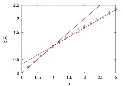
Figure 5: Scaling exponents $\chi(p)$ for the moments of the exit times $\langle T^{p}(\delta v)\rangle$. The lines represent the bifractal prediction (7). The error bars on the exponents have been estimated by evaluating differences in $\chi(p)$ changing the fitting interval.

In conclusions, we have analyzed single-particle dispersion in the two-dimensional Bolgiano turbulent convection. A remarkable property of this turbulent regime is that the single-particle dispersion turns out to be dominated by the large-scale eddies whose contribution to velocity fluctuations behaves linearly with time. A completely different scenario thus emerge with respect to the classical single-particle dispersion in a flow which displays the standard K41 phenomenology. The Bolgiano–Obukhov contribution to the scaling of Lagrangian velocity increments thus results undetectable by standard Lagrangian structure functions. To disentangle its effect from the (trivial) one played by large scales, we have exploited a method of analysis based on exit-time statistics for signals having more than smooth fluctuations. The obtained results clearly permit to identify the contribution of ”local” eddies to the Lagrangian velocity fluctuations.

This work has been supported by COFIN 2005 project n. 2005027808 and by CINFAI consortium (A.M.).

References

- (1) S.B. Pope, Annu. Rev. Fluid Mech. “Lagrangian PDF methods for turbulent flows” 26, 23 (1994).
- (2) B. Sawford, “Turbulent relative dispersion” Annu. Rev. Fluid Mech. 33, 289 (2001).
- (3) P.K. Yeung, “Lagrangian investigations of turbulence” Annu. Rev. Fluid Mech. 34, 115 (2002).
- (4) G. Falkovich, K. Gawedzki and M. Vergassola, “Particles and fields in fluid turbulence” Rev. Mod. Phys. 73, 913 (2001).
- (5) A. La Porta, G. A. Voth, A. M. Crawford, J. Alexander and E. Bodenschatz, “Fluid particle accelerations in fully developed turbulence” Nature 409, 1017 (2001).
- (6) N. Mordan, P. Metz, O. Michel, and J.F. Pinton, “Measurement of Lagrangian velocity in fully developed turbulence” Phys. Rev. Lett. 87, 214501 (2001).
- (7) S. Ott and J. Mann, “An experimental investigation of the relative diffusion of particle pairs in three-dimensional turbulent flow” J. Fluid Mech. 422, 207 (2000).
- (8) P.K. Yeung, “Lagrangian characteristics of turbulence and scalar transport in direct numerical simulations” J. Fluid Mech. 427, 241 (2001).
- (9) L. Biferale, G. Boffetta, A. Celani, A. Lanotte and F. Toschi, “Particle trapping in three-dimensional fully developed turbulence”, Phys. Fluids 17, 021701 (2005).
- (10) E.D. Siggia, “High Rayleigh number convection,” Annu. Rev. Fluid Mech. 26, 137 (1994).
- (11) A. Celani, A. Mazzino and M. Vergassola, “Thermal plume turbulence”, Phys. Fluids, 13 2133 (2001).
- (12) A. Monin and A. Yaglom, “Statistical fluid mechanics” (Cambridge, MA: MIT Press, 1975).
- (13) L. Biferale, M. Cencini, A. Lanotte, D. Vergni and A. Vulpiani, “Inverse statistics of smooth signals: the case of two-dimensional turbulence”, Phys. Rev. Lett. 87, 124501 (2001).
- (14) V. Artale, G. Boffetta, A. Celani, M. Cencini and A. Vulpiani, “Dispersion of passive tracers in closed basins: Beyond the diffusion coefficient”, Phys. Fluids 9, 3162 (1997)