Relations for zeros of special polynomials associated to the Painlevé equations

Abstract

A method for finding relations for the roots of polynomials is presented. Our approach allows us to get a number of relations for the zeros of the classical polynomials and for the roots of special polynomials associated with rational solutions of the Painlevé equations. We apply the method to obtain the relations for the zeros of several polynomials. They are: the Laguerre polynomials, the Yablonskii - Vorob’ev polynomials, the Umemura polynomials, the Ohyama polynomials, the generalized Okamoto polynomials, and the generalized Hermite polynomials. All the relations found can be considered as analogues of generalized Stieltjes relations.

Keywords: Special polynomials, Rational solutions, Stieltjes relations, the Painlevé equation, power expansion

PACS: 02.30.Hq - Ordinary differential equations

1 Introduction

In 1885 Stieltjes [1, 2] suggested the following relations for the roots of the Hermite polynomials [3, 4]

$$\begin{gathered}\sum_{k\neq j}^{n}\left(z_{j}-z_{k}\right)^{-1}-z_{j}=0,\,\,\,\,(j=1,...,n)\end{gathered}$$ (1.1)

These relations can be considered as the equilibrium configurations of $n$ particles on the line interecting pairwise with a repulse logarithmic potential in the harmonic field [4, 5, 6].

In this paper we introduce a new approach for finding relations like (1.1) satisfied by the roots of polynomials, which can be generated by a differential equation. We demonstrate our approach to get relations for the roots of the Laguerre polynomials and for the roots of special polynomials associated with rational solutions of the second, the third, and the fourth Painlevé equations.

The six Painlevé equations $(P_{1}-P_{6})$ were picked out by Painlevé and his student Gambier from a certain class of second - order differential equations as equations whose general solutions on the one hand, do not have movable critical points and on the other hand, cannot be expressed through known elementary or special functions. In other words they define new transcendental functions. However, the equations $P_{2}-P_{6}$ possess hierarchies of rational and algebraic solutions at certain values of the parameters. It turned out that such solutions could be described using families of special polynomials. The history of this question is as follows.

A. I. Yablonskii and A. P. Vorob’ev were the first who expressed the rational solutions of $P_{2}$ via the logarithmic derivative of the polynomials, which now go under the name of the Yablonskii – Vorob’ev polynomials [7, 8]. Later K. Okamoto suggested special polynomials for certain rational solutions of $P_{4}$ [9]. H. Umemura derived analogous polynomials for some rational and algebraic solutions of $P_{3}$ and $P_{5}$ [10]. All these polynomials possess a number of interesting properties. For example, they can be expressed in terms of Schur polynomials. Besides that the polynomials arise as the so – called tau-functions and satisfy recurrence relations of Toda type. Recently these polynomials have been intensively studied [11, 12, 13].

Apart from rational and algebraic solutions $P_{2}-P_{6}$ possess one – parameter families of solutions expressible in terms of the classical special functions. In particular cases these special function solutions are reduced to classical orthogonal polynomials and, consequently give rational solutions of the Painlevé equation in question. For $P_{4}$ these polynomials are Hermite polynomials, for $P_{3}$ and $P_{5}$ Laguerre polynomials and for $P_{6}$ Jacobi polynomials.

Not long ago P. A. Clarkson and E. L. Mansfield suggested special polynomials for the equations of the $P_{2}$ hierarchy [14]. Also they studied the location of their roots in the complex plane and showed that the roots have a very regular structure.

The textbook [15] characterizes the Painlevé equations as ”the most important nonlinear ordinary differential equations” and states that ”many specialists believe that during the twenty-first century the Painlevé equations will become new members of the community of special functions” [16].

In this paper we study the relations for the zeros of the following equations

$$\begin{gathered}yy_{{{zzzz}}}-4\,y_{{z}}y_{{{zzz}}}+3\,{y_{{{zz}}}}^{2}-z\left(yy_{{{zz}}}-{y_{{z}}}^{2}\right)-yy_{{z}}=0,\end{gathered}$$ (1.2)

$$\begin{gathered}z^{2}\,(y\,y_{zzzz}-4\,y_{z}\,y_{zzz}+3\,y_{zz}^{2})+2\,z\,(y\,y_{zzz}-y_{z}\,y_{zz})\\ -4\,z\,(z+\mu)(\,y\,y_{zz}-y_{z}^{2})-2\,y\,y_{zz}+4\,\mu\,y\,y_{z}-2\,n\,(n+1)\,y^{2}=0,\end{gathered}$$ (1.3)

$$\begin{gathered}z^{3}\,(y\,y_{zzzz}-4\,y_{z}\,y_{zzz}+3\,y_{zz}^{2})-6\,z^{2}\,(y\,y_{zzz}-y_{z}\,y_{zz})\\ -12\,z\,(z^{4}-3\,n-1)(\,y\,y_{zz}-y_{z}^{2})-9\,z\,(y\,y_{zz}+y_{z}^{2})\\ +3(12\,z^{4}-16\,n\,z^{2}+12\,n+7)y\,y_{z}\\ -24\,n\,z\,((n+3)\,z^{2}-3\,n-1)\,y^{2}=0,\end{gathered}$$ (1.4)

$$\begin{gathered}y\,y_{zzzz}-4\,y_{z}\,y_{zzz}+3\,y_{zz}^{2}+\frac{4}{3}\,z^{2}\,(y\,y_{zz}-y_{z}^{2})+4\,z\,y\,y_{z}\\ -\frac{8}{3}\,(m^{2}+n^{2}+m\,n-m-n)\,y^{2}=0,\end{gathered}$$ (1.5)

$$\begin{gathered}y\,y_{zzzz}-4\,y_{z}\,y_{zzz}+3\,y_{zz}^{2}-4(z^{2}+2n-2m)\,(y\,y_{zz}-y_{z}^{2})\\ +4\,z\,y\,y_{z}-8\,m\,n\,y^{2}=0.\end{gathered}$$ (1.6)

It is known [11] that particular solutions of equation (1.2) are the Yablonskii - Vorob’ev polynomials. Rational solutions of the second Painlevé equation can be expressed as the logarithmic derivative of these polynomials. In this work using our approach we obtain some new relations for the zeros of these polynomials. These relations explain a very regular location of the zeros in the complex plain.

The equations (1.3) and (1.4) in their turn possess polynomial solutions, i.e. the Umemura polynomials and the Ohyama polynomials [12], accordingly. Rational solutions of the third Painlevé equation can be obtained with the help of these polynomials. The general form of these polynomials is not known at present but using the method of our recent works [18, 17] one can solve this problem and can get the general form for these polynomials. However here we present new additional correlations for the zeros of these polynomials.

The equations (1.5) and (1.6) also admit polynomial solutions, which are the generalized Okamoto polynomials and the generalized Hermite polynomials, respectively [13]. Rational solutions of the fourth Painlevé equation can be expressed via logarithmic derivative of these polynomials. The general form of these polynomials is not known as well. In this work new correlations for the zeros of these polynomials are obtained.

This paper is organized as follows. In section 2 we present the method of finding the relations for the roots of the polynomials. In this section we also apply our approach on the example to have the relations for the roots of the Laguerre polynomials. Sections 2, 3, 4 and 5 are devoted to finding the relations for the zeros of the Yablonskii - Vorob’ev polynomials, of the Umemura polynomials, of the Ohyama polynomials, of the generalized Okamoto polynomials and of the generalized Hermite polynomials. All these polynomials are associated with rational solutions of the second, the third and the fourth Painlevé equations.

2 Method applied

Let us assume that we have an n-linear (linear, bilinear etc) equation of order $M$

$$\begin{gathered}E_{1}\left(y,y_{z},y_{zz},...,z\right)=0.\end{gathered}$$ (2.1)

In addition suppose that this equation admits polynomial solution $y(z)=q(z)$ of degree $p$. The transformation

$$\begin{gathered}w(z)=\frac{y_{z}}{y}\end{gathered}$$ (2.2)

maps solutions of the equation (2.1) into solutions of the nonlinear equation

$$\begin{gathered}E_{2}\left(w,w_{z},w_{zz},...,z\right)=0.\end{gathered}$$ (2.3)

Note that the degree of (2.3) is $M-1$. Under such transformation the polynomial $q(z)$ becomes the rational function

$$\begin{gathered}w(z)=\sum_{k=1}^{\tilde{p}}\frac{e_{k}}{z-z_{k}},\end{gathered}$$ (2.4)

where $z_{j}$ is a root of $q(z)$ of degree $e_{j}$ and

$$\begin{gathered}p=\sum_{j=1}^{\tilde{p}}e_{j},\end{gathered}$$ (2.5)

i.e. $\tilde{p}$ is the number of distinct roots. The rational function (2.4) can be expanded in a neighborhood of a pole $z_{j}$ and this gives

$$\begin{gathered}w(z)=\frac{e_{j}}{z-z_{j}}-\sum_{m=0}^{\infty}\left(\sum_{k\neq i}\frac{e_{k}}{(z_{k}-z_{j})^{m+1}}\right)(z-z_{j})^{m},\\ \\ 0<\mid z-z_{j}\mid<\min_{k\neq j}\mid z_{k}-z_{j}\mid\end{gathered}$$ (2.6)

At the same time we can find expansions of solution $w(z)$ near movable singular point $z_{0}$ using the Painlevé test [19, 20, 21, 22] or methods of power geometry[23, 24, 25, 27, 26]. The result of calculations for the rational function $w(z)$ takes the form

$$\begin{gathered}w(z)=\sum_{m=0}^{\infty}c_{m}(z-z_{0})^{m-1},\end{gathered}$$ (2.7)

Assuming $z_{0}=z_{j}$, $c_{0}=e_{j}$ and comparing this series with (2.6) yields

$$\begin{gathered}\forall j:\quad\sum_{k\neq i}\frac{e_{k}}{(z_{k}-z_{j})^{m+1}}=-c_{m},\quad m>0.\end{gathered}$$ (2.8)

We are going to use correlations (2.8) for finding some relations of the zeros of the above mentioned polynomials, which are associated with the rational solutions of the second, the third, and the fourth Painlevé equations.

Let us demonstrate our approach by the example of the Laguerre polynomials $L_{n}^{(\alpha)}(z)$. They satisfy the following second-order linear differential equation

$$\begin{gathered}z\,y_{zz}+(\alpha+1-z)\,y_{z}+n\,y=0.\end{gathered}$$ (2.9)

Substituting $y_{z}=w(z)\,y(z)$, $y_{zz}=(w_{z}+w^{2})y$ into (2.9) and dividing the result by $y(z)$ we obtain the first-order nonlinear differential of the form

$$\begin{gathered}z\,w_{z}+z\,w^{2}+\left(\alpha+1-z\right)w+n=0.\end{gathered}$$ (2.10)

Taking the Painlevé methods into account we have the power expansions for rational solution of equation (2.10) near singular point $z=z_{0}$ $(z_{0}\neq 0)$ in the form

$$\begin{gathered}w(z)=\frac{1}{z-{z_{0}}}-\frac{1}{2}\,{\frac{\alpha+1-{z_{0}}}{{z_{0}}}}+\frac{1}{{{12\,z_{0}}}^{2}}\,[\,6\,\alpha+5-2\,{z_{0}}-2\,\alpha\,{z_{0}}+\\ \\ +{{z_{0}}}^{2}-4\,n{z_{0}}+{\alpha}^{2}\,]\left(z-{z_{0}}\right)-\frac{1}{8{{z_{0}}}^{3}}\,[\,4\,\alpha+{\alpha}^{2}+3-\alpha\,{z_{0}}-2\,n{z_{0}}-\\ \\ -{z_{0}}\,]\left(z-{z_{0}}\right)^{2}-{\frac{1}{720{{z_{0}}}^{4}}}\,[\,76\,\alpha\,{z_{0}}-360\,\alpha-8\,n{z_{0}}\,{\alpha}^{2}+2\,{{z_{0}}}^{2}+\\ \\ +152\,n{z_{0}}-110\,{\alpha}^{2}-4\,{\alpha}^{2}{z_{0}}+8\,\alpha\,{{z_{0}}}^{2}+16\,n{{z_{0}}}^{2}-4\,{{z_{0}}}^{3}-251+\\ \\ +{{z_{0}}}^{4}+{\alpha}^{4}-8\,{{z_{0}}}^{3}n+6\,{\alpha}^{2}{{z_{0}}}^{2}-4\,\alpha\,{{z_{0}}}^{3}-4\,{\alpha}^{3}{z_{0}}+\\ \\ +16\,{n}^{2}{{z_{0}}}^{2}+16\,\alpha\,{{z_{0}}}^{2}n+76\,{z_{0}}\,]\left(z-{z_{0}}\right)^{3}+...\end{gathered}$$ (2.11)

Comparing the power expansion (2.11) with (2.6) we have the following relations for the zeros of the Laguerre polynomials in the case $z_{j}\neq 0$

$$\begin{gathered}\sum_{k\neq j}^{\tilde{n}}\frac{e_{k}}{(z_{k}-z_{j})}-\frac{\alpha+1}{2\,z_{j}}+\frac{1}{2}=0,\end{gathered}$$ (2.12)

$$\begin{gathered}\sum_{k\neq j}^{\tilde{n}}\frac{e_{k}}{(z_{k}-z_{j})^{2}}+\frac{\alpha^{2}+6\,\alpha+5}{12\,z_{j}^{2}}-\frac{1+\alpha+n}{6\,z_{j}}+\frac{1}{12}=0,\end{gathered}$$ (2.13)

$$\begin{gathered}\sum_{k\neq j}^{\tilde{n}}\frac{e_{k}}{(z_{k}-z_{j})^{3}}-\frac{\alpha^{2}+4\,\alpha+3}{8\,z_{j}^{3}}+\frac{1+\alpha+2\,n}{8\,z_{j}^{2}}=0\end{gathered}$$ (2.14)

In this expressions $\tilde{n}$ makes sense of $\tilde{p}$ and $e_{k}=1$, $z_{k}\neq 0$. It is known that $z=0$ is the root of $L_{n}^{(\alpha)}(z)$ if and only if $\alpha=-l$ $(1\leq l\leq n)$. Then in this case the asymptotic series in a neighborhood of $z=0$ is

$$\begin{gathered}w(z)={\frac{l}{z}}-{\frac{n-l}{l+1}}-{\frac{\left(n-l\right)\left(n+1\right)z}{\left(l+2\right)\left(l+1\right)^{2}}}\left[1+\frac{(2\,n+1-l)z}{\left(l+3\right)\left(l+1\right)}\right.\\ \left.+\frac{(5\,{n}^{2}l+11\,{n}^{2}+11\,n-5\,n{l}^{2}-6\,nl+2-6\,l+{l}^{3}-{l}^{2}){z}^{2}}{(l+3)(l+4)(l+2)(l+1)^{2}}+o(z^{2})\right]\end{gathered}$$ (2.15)

There are no arbitrary constants in this expansion as the critical number $k$ is $k=-l-1<-1$. Without loss of generality let us suppose that $z=0$ is the first in the set of roots. Comparing the series (2.15) with (2.6) we see that the order of the root $z=0$ is $l$ and

$$\begin{gathered}\sum_{k=2}^{\tilde{n}}\frac{1}{z_{k}}-{\frac{n-l}{l+1}}=0,\end{gathered}$$ (2.16)

$$\begin{gathered}\sum_{k=2}^{\tilde{n}}\frac{1}{z_{k}^{2}}-{\frac{\left(n-l\right)\left(n+1\right)}{\left(l+2\right)\left(l+1\right)^{2}}}=0,\end{gathered}$$ (2.17)

$$\begin{gathered}\sum_{k=2}^{\tilde{n}}\frac{1}{z_{k}^{3}}-{\frac{\left(n-l\right)\left(n+1\right)(2\,n+1-l)}{\left(l+2\right)(l+3)\left(l+1\right)^{3}}}=0\end{gathered}$$ (2.18)

We would like to note that in such a way one can find analogous relations for some other polynomials.

3 Relations for the zeros of the Yablonskii - Vorob’ev polynomials

The transformation (2.2) maps solutions of the equation (1.2) into solutions of the third-order nonlinear differential equation

$$\begin{gathered}w_{{{zzz}}}+6\,{w_{{z}}}^{2}-zw_{{z}}-w=0.\end{gathered}$$ (3.1)

The Laurent expansion of its solution $w(z)$ in a neighborhood of a movable pole $z_{0}$ is the following

$$\begin{gathered}w(z)=\frac{1}{(z-z_{0})}+{a_{1}}+\frac{{z_{0}}}{12}\,\left(z-z_{{0}}\right)-\left({\frac{{{z_{0}}}^{2}}{720}}\,+\frac{{a_{1}}}{30}\right)\left(z-z_{{0}}\right)^{3}-\\ \\ -{\frac{{z_{0}}}{144}}\,\,\left(z-z_{{0}}\right)^{4}+{a_{6}}\,\left(z-z_{{0}}\right)^{5}-\left({\frac{{{z_{0}}}^{2}}{8640}}\,+{\frac{{a_{1}}}{360}}\,\right)\left(z-z_{{0}}\right)^{6}+...\end{gathered}$$ (3.2)

The Yablonskii - Vorob’ev polynomials $Q_{n}(z)$ are monic polynomials of degree $n(n+1)/2$ with simple roots. Then from power expansion (3.2) we obtain the following relations for the zeros of $Q_{n}(z)$

$$\begin{gathered}\sum_{k\neq j}^{n(n+1)/2}\frac{1}{(z_{k}-z_{j})}+a_{1}=0,\end{gathered}$$ (3.3)

$$\begin{gathered}\sum_{k\neq j}^{n(n+1)/2}\frac{1}{(z_{k}-z_{j})^{2}}+\frac{z_{j}}{12}\,=0,\end{gathered}$$ (3.4)

$$\begin{gathered}\sum_{k\neq j}^{n(n+1)/2}\frac{1}{(z_{k}-z_{j})^{3}}=0,\end{gathered}$$ (3.5)

$$\begin{gathered}\sum_{k\neq j}^{n(n+1)/2}\frac{1}{(z_{k}-z_{j})^{4}}+\frac{{1}}{30}\,\sum_{k\neq j}^{n(n+1)/2}\frac{1}{(z_{k}-z_{j})}-{\frac{{{z_{j}}}^{2}}{720}}\,=0,\end{gathered}$$ (3.6)

$$\begin{gathered}\sum_{k\neq j}^{n(n+1)/2}\frac{1}{(z_{k}-z_{j})^{5}}-\frac{z_{j}}{144}\,=0,\end{gathered}$$ (3.7)

$$\begin{gathered}\sum_{k\neq j}^{n(n+1)/2}\frac{1}{(z_{k}-z_{j})^{6}}+a_{6}=0,\end{gathered}$$ (3.8)

$$\begin{gathered}\sum_{k\neq j}^{n(n+1)/2}\frac{1}{(z_{k}-z_{j})^{7}}+{\frac{1}{360}}\,\sum_{k\neq j}^{n(n+1)/2}\frac{1}{(z_{k}-z_{j})}-{\frac{{{z_{j}}}^{2}}{8640}}\,=0\end{gathered}$$ (3.9)

In this expressions the coefficients $a_{1}$ and $a_{6}$ depend on $n$ and $z_{j}$. Further the coefficient $a_{6}$ can be calculated if we note that the equation (3.1) possesses the first integral

$$\begin{gathered}w_{zz}^{2}-\frac{1}{2}w_{zz}+4w_{z}^{3}-zw_{z}^{2}-2ww_{z}+\frac{1}{2}zw+C=0.\end{gathered}$$ (3.10)

The latter equation has rational solutions in the form $w(z;n)=d_{z}\ln(Q_{n}(z))$ if $C=-n(n+1)/4$. The Laurent expansion of $w(z;n)=d_{z}\ln(Q_{n}(z))$ coincide with (3.2) accurate to the value of $a_{6}$, which is no longer arbitrary

$$\begin{gathered}a_{{6}}={\frac{1}{30240}}\,{{\it z_{j}}}^{3}-{\frac{1}{280}}-{\frac{1}{420}}\,{\it z_{j}}\,a_{{1}}+{\frac{1}{560}}\,n+{\frac{1}{560}}\,{n}^{2}.\end{gathered}$$ (3.11)

We do not present here the Yablonskii - Vorob’ev polynomials. They were obtained before[7, 8, 11, 17]. Let us give here only the polynomial $Q_{7}(z)$. That is

$$\begin{gathered}Q_{7}\left(z\right)=[{z}^{27}+504\,{z}^{24}+75600\,{z}^{21}+5174400\,{z}^{18}+62092800\,{z}^{15}+\\ +13039488000\,{z}^{12}-828731904000\,{z}^{9}-\\ -49723914240000\,{z}^{6}-3093932441600000]z.\end{gathered}$$ (3.12)

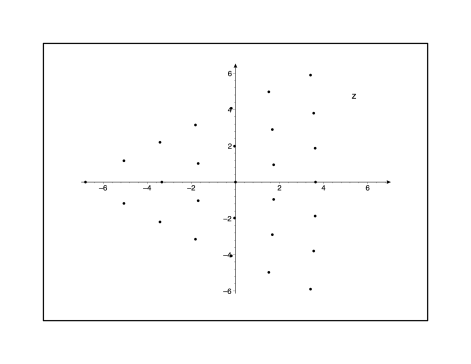
Figure 1: Configuration of zeros for the Yablonskii - Vorob’ev polynomials $Q_{7}(z)$

The configuration of the zeros for the Yablonskii - Vorob’ev polynomial $Q_{7}(z)$ is illustrated in the Figure 1.

4 Relations for the zeros of the Umemura polynomials

Using the formula $y_{z}=w(z)\,y(z)$ we can transform equation (1.3) to the following third-order nonlinear equation

$$\begin{gathered}{z}^{2}w_{{{zzz}}}+6\,{z}^{2}{w_{{z}}}^{2}+2\,z\,w_{{{zz}}}+4\,zww_{{z}}-4\,{z}^{2}w_{{z}}-4\,z\,w_{{z}}\mu-2\,w_{{z}}-\\ \\ -2\,{w}^{2}+4\,\mu\,w-2\,{n}^{2}-2\,n=0.\end{gathered}$$ (4.1)

With the help of the Painlevé methods [19] we find the power expansion of its solutions $w(z)$ near movable singularity $z_{0}\neq 0$

$$\begin{gathered}w(z)=\frac{1}{z-z_{0}}+a_{{1}}-{\frac{\left(a_{{1}}-z_{{0}}-\mu\right)}{3\,z_{{0}}}}\left(z-z_{{0}}\right)-\frac{1}{45{{z_{{0}}}^{3}}}\,[\,4\,{a_{{1}}}^{2}z_{{0}}-\\ \\ -2\,{z_{{0}}}^{2}a_{{1}}-8\,\mu\,a_{{1}}z_{{0}}+3\,{n}^{2}z_{{0}}+3\,z_{{0}}-9\,a_{{1}}+9\,\mu+3\,nz_{{0}}+2\,\mu\,{z_{{0}}}^{2}+\\ \\ +{\mu}^{2}z_{{0}}+{z_{{0}}}^{3}]\left(z-z_{{0}}\right)^{3}+\frac{1}{9{z_{{0}}}^{4}}\,[\,\mu\,{z_{{0}}}^{2}-{z_{{0}}}^{2}a_{{1}}+2\,{a_{{1}}}^{2}z_{{0}}-4\,\mu\,a_{{1}}z_{{0}}+\\ \\ +{\mu}^{2}z_{{0}}+3\,\mu+{n}^{2}z_{{0}}+z_{{0}}-3\,{a_{1}}+nz_{{0}}\,]\left(z-z_{{0}}\right)^{4}+a_{{6}}\left(z-z_{{0}}\right)^{5}+...\end{gathered}$$ (4.2)

Making use of the expansion near infinity for $w(z)$ we easily find the degree $p$ of the Umemura polynomials $p=n(n+1)/2$. Proceeding in the way stated in section 2 we obtain the following relations for the zeros of the Umemura polynomials in the case $z_{j}\neq 0$

$$\begin{gathered}\sum_{k\neq j}^{\tilde{p}}\frac{e_{k}}{(z_{k}-z_{j})}+a_{1}=0,\end{gathered}$$ (4.3)

$$\begin{gathered}\sum_{k\neq j}^{\tilde{p}}\frac{e_{k}}{(z_{k}-z_{j})^{2}}-{\frac{\left(a_{{1}}-\mu\right)}{3\,z_{{j}}}}+\frac{1}{3}=0,\end{gathered}$$ (4.4)

$$\begin{gathered}\sum_{k\neq j}^{\tilde{p}}\frac{e_{k}}{(z_{k}-z_{j})^{3}}=0,\end{gathered}$$ (4.5)

$$\begin{gathered}\sum_{k\neq j}^{\tilde{p}}\frac{e_{k}}{(z_{k}-z_{j})^{4}}-\frac{(\mu-a_{1})}{5\,z_{j}^{3}}-\frac{2\,(\mu-a_{1})}{45\,z_{j}}-\frac{1}{45}-\\ \\ -\frac{(\,4\,{a_{{1}}}^{2}-8\,\mu\,a_{{1}}+\mu^{2}+3+3\,n+3\,n^{2})}{45\,{{z_{{j}}}^{2}}}\,=0.\end{gathered}$$ (4.6)

Here $e_{k}=1$ for all $z_{k}\neq 0$. Substituting $a_{1}$ from (4.3) into (4.4) we obtain

$$\begin{gathered}\sum_{k\neq j}^{n}\frac{1}{(z_{k}-z_{j})^{2}}+\frac{1}{3\,z_{j}}\,\sum_{k\neq j}^{n}\frac{1}{z_{k}-z_{j}}+\frac{\mu}{3\,z_{j}}+\frac{1}{3}=0.\end{gathered}$$ (4.7)

The Umemura polynomials $Q_{5}(z)$ takes the form [13]

$$\begin{gathered}Q_{{5}}(z)={z}^{15}-135\,{z}^{14}+8505\,{z}^{13}-331380\,{z}^{12}+8921745\,{z}^{11}-\\ -175642425\,{z}^{10}+2609560800\,{z}^{9}-29764778400\,{z}^{8}+\\ +262512608400\,{z}^{7}-1788313917600\,{z}^{6}+9322366561200\,{z}^{5}-\\ -36474213006000\,{z}^{4}+103536532638000\,{z}^{3}-200979491328000\,{z}^{2}+\\ +238097325312000\,z-129459762432000\end{gathered}$$ (4.8)

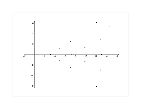
Figure 2: Configuration of zeros for the Umemura polynomial $Q_{5}(z)$ at $\mu=16$

The configuration of the zeros for the Umemura polynomial $Q_{5}(z)$ is demonstrated in the Figure 2.

5 Relations for the zeros of the Ohyama polynomials

Using $y_{z}=w(z)\,y$ we have from (1.4) the following third-order differential equation

$$\begin{gathered}{z}^{3}w_{{{zzz}}}-6\,{z}^{2}w_{{{zz}}}+6\,{z}^{3}{w_{{z}}}^{2}+\left(-12\,{z}^{2}w-12\,{z}^{5}+36\,nz+3\,z\right)w_{{z}}-\\ -18\,z{w}^{2}+\left(21+36\,{z}^{4}-48\,n{z}^{2}+36\,n\right)w+24\,nz-\\ -24\,{n}^{2}{z}^{3}-72\,n{z}^{3}+72\,{n}^{2}z=0.\end{gathered}$$ (5.1)

The power expansion for the solutions of equation (5.1) in a neighborhood of a pole $z=z_{0}$ $(z_{0}\neq 0)$ is

$$\begin{gathered}w(z)=\frac{1}{z-z_{0}}+a_{{1}}+\frac{1}{{4\,z_{{0}}}^{2}}{{\left(4\,a_{{1}}z_{{0}}-7-12\,n+4\,{z_{{0}}}^{4}\right)}{}}\left(z-z_{{0}}\right)+\\ \\ +\frac{1}{{8\,z_{{0}}}^{3}}{{\left(21-16\,a_{{1}}z_{{0}}+36\,n+20\,{z_{{0}}}^{4}-16\,n{z_{{0}}}^{2}\right)}{}}\left(z-{z_{0}}\right)^{2}-\\ \\ -{\frac{1}{80{{z_{{0}}}^{4}}}}\,[\,64\,{n}^{2}{z_{{0}}}^{4}+64\,{z_{{0}}}^{2}{a_{{1}}}^{2}-64\,a_{{1}}{z_{{0}}}^{5}+96\,n{z_{{0}}}^{4}+120\,{z_{{0}}}^{4}+144\,{n}^{2}+\\ \\ +128\,na_{{1}}{z_{{0}}}^{3}+16\,{z_{{0}}}^{8}+301-320\,n{z_{{0}}}^{2}-192\,na_{{1}}z_{{0}}-192\,{n}^{2}{z_{{0}}}^{2}-\\ \\ -320\,a_{{1}}z_{{0}}+600\,n\,]\left(z-z_{{0}}\right)^{3}+\frac{1}{32{{z_{{0}}}^{5}}}\,[161-64\,{z_{{0}}}^{6}n+64\,{n}^{2}{z_{{0}}}^{4}+\\ \\ +64\,{z_{{0}}}^{2}{a_{{1}}}^{2}-64\,a_{{1}}{z_{{0}}}^{5}+96\,n{z_{{0}}}^{4}+104\,{z_{{0}}}^{4}+144\,{n}^{2}+128\,na_{{1}}{z_{{0}}}^{3}+\\ \\ +16\,{z_{{0}}}^{8}-208\,n{z_{{0}}}^{2}-192\,na_{{1}}z_{{0}}-192\,{n}^{2}{z_{{0}}}^{2}-208\,a_{{1}}z_{{0}}+\\ \\ +360\,n]\left(z-z_{{0}}\right)^{4}+a_{{6}}\left(z-z_{{0}}\right)^{5}+...\end{gathered}$$ (5.2)

The degree of the Ohyama polynomial can be obtained with the help of the expansion of $w(z)$ near infinity and equals $n(n+3)/2$. From power expansion (5.3) we obtain the following relations for the roots of the Ohyama polynomials in the case $z_{j}\neq 0$

$$\begin{gathered}\sum_{k\neq j}^{\tilde{p}}\frac{e_{k}}{z_{k}-z_{j}}+a_{1}=0,\end{gathered}$$ (5.3)

$$\begin{gathered}\sum_{k\neq j}^{\tilde{p}}\frac{e_{k}}{(z_{k}-z_{j})^{2}}+z_{j}^{2}+\frac{a_{1}}{z_{j}}-\frac{(7+12\,n)}{4\,z_{j}^{2}}=0,\end{gathered}$$ (5.4)

$$\begin{gathered}\sum_{k\neq j}^{\tilde{p}}\frac{e_{k}}{(z_{k}-z_{j})^{3}}+\frac{5}{2}\,z_{j}-\frac{2\,n}{z_{j}}-\frac{2\,a_{1}}{z_{j}^{2}}+\frac{(21+36\,n)}{8\,z_{j}^{3}}=0,\end{gathered}$$ (5.5)

$$\begin{gathered}\sum_{k\neq j}^{\tilde{p}}\frac{e_{k}}{(z_{k}-z_{j})^{4}}-\frac{z_{j}^{4}}{5}+\frac{4\,a_{1}}{5}\,z_{j}-\frac{(8\,n^{2}+12\,n+15)}{10}-\frac{8\,n\,a_{1}}{5\,z_{j}}-\\ \\ -\frac{(4\,a_{1}^{2}-20\,n-12\,n^{2})}{5\,z_{j}^{2}}+\frac{4\,a_{1}\,(3\,n+4)}{5\,z_{j}^{3}}-{\frac{(144\,{n}^{2}+301+600\,n)}{80{{z_{{j}}}^{4}}}}=0\end{gathered}$$ (5.6)

In this expressions $e_{k}=1$ if $z_{k}\neq 0$. Substituting $a_{1}$ from (5.3) into (5.4) we have

$$\begin{gathered}\sum_{k\neq j}^{\tilde{p}}\frac{e_{k}}{(z_{k}-z_{j})^{2}}-\frac{1}{z_{j}}\,\sum_{k\neq j}^{\tilde{p}}\frac{e_{k}}{(z_{k}-z_{j})}+z_{j}^{2}-\frac{{{\left(7+12\,n\right)}}}{{4\,z_{{j}}}^{2}}=0.\end{gathered}$$ (5.7)

The Ohyama polynomial $P_{7}(z)$ can be written in the form [13]

$$\begin{gathered}P_{7}(z)={z}^{11}[{z}^{24}-56\,{z}^{22}+1470\,{z}^{20}-23800\,{z}^{18}+263375\,{z}^{16}-\\ -2088240\,{z}^{14}+12105940\,{z}^{12}-51466800\,{z}^{10}+158533375\,{z}^{8}-\\ -343343000\,{z}^{6}+493643150\,{z}^{4}-421821400\,{z}^{2}+163788625]\end{gathered}$$ (5.8)

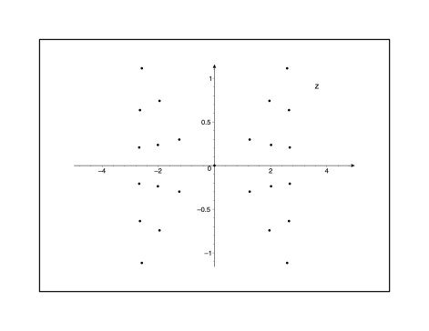
Figure 3: Configuration of zeros for the Ohyama polynomial $P_{7}(z)$

The configuration of the zeros for the Ohyama polynomial $P_{7}(z)$ is presented in the Figure 3.

6 Relations for the zeros of the generalized Okamoto polynomials

Substituting the following expression $y_{z}=w(z)y$ into (1.5) sufficient amount of times we get

$$\begin{gathered}w_{{{zzz}}}+6\,{w_{{z}}}^{2}+\frac{4}{3}\,{z}^{2}w_{{z}}+4\,z\,w+\frac{8}{3}\,\left({m}^{2}+\,{n}^{2}+\,mn-\,m-\,n\right)=0.\end{gathered}$$ (6.1)

The Laurent expansion for solutions of this equation near movable singularity $z=z_{0}$ is

$$\begin{gathered}w(z)=\frac{1}{z-z_{0}}+a_{{1}}-\frac{{z_{{0}}}^{2}}{9}\,\left(z-z_{{0}}\right)+\frac{z_{{0}}}{18}\,\left(z-z_{{0}}\right)^{2}+\\ \\ +\left({\frac{4}{45}}\,n-{\frac{4}{45}}\,{m}^{2}+\frac{2z_{{0}}a_{{1}}}{15}\,-{\frac{4}{45}}\,mn+{\frac{4}{45}}\,m-{\frac{1}{405}}\,{z_{{0}}}^{4}+{\frac{4}{45}}-{\frac{4}{45}}\,{n}^{2}\right)\\ \\ \left(z-z_{{0}}\right)^{3}+\left(\frac{a_{{1}}}{6}-{\frac{5}{162}}\,{z_{{0}}}^{3}\right)\left(z-z_{{0}}\right)^{4}+{a_{6}}\,\left(z-z_{{0}}\right)^{5}+{\frac{z_{{0}}}{9720}}\,[\,8\,{z_{{0}}}^{4}-\\ \\ -432\,z_{{0}}a_{{1}}+288\,mn-288\,n+288\,{m}^{2}-363+288\,{n}^{2}-288\,m]\left(z-z_{{0}}\right)^{6}\end{gathered}$$ (6.2)

Then relations for the zeros of the generalized Okamoto polynomials can be written as

$$\begin{gathered}\sum_{k\neq j}^{p}\frac{1}{(z_{k}-z_{j})}+a_{1}=0,\end{gathered}$$ (6.3)

$$\begin{gathered}\sum_{k\neq j}^{p}\frac{1}{(z_{k}-z_{j})^{2}}-\frac{z_{j}^{2}}{9}=0,\end{gathered}$$ (6.4)

$$\begin{gathered}\sum_{k\neq j}^{p}\frac{1}{(z_{k}-z_{j})^{3}}+\frac{z_{j}}{18}=0,\end{gathered}$$ (6.5)

$$\begin{gathered}\sum_{k\neq j}^{p}\frac{1}{(z_{k}-z_{j})^{4}}-{\frac{{z_{{j}}}^{4}}{405}}\,\,+\,\frac{2\,a_{{1}}\,z_{{j}}}{15}+\\ \\ +\frac{4}{45}\,\left(1+m+n-{m}^{2}-m\,n-{n}^{2}\,\right)=0,\end{gathered}$$ (6.6)

where the degree $p$ of the generalized Okamoto polynomial $P_{n,m}(z)$ is $p=m^{2}+n^{2}+mn-m-n$.

The generalized Okamoto polynomials $P_{4,4}(z)$ takes the form[12]

$$\begin{gathered}P_{4,4}\left(z\right)={z}^{40}-{\frac{1755}{2}}\,{z}^{36}+{\frac{4238325}{16}}\,{z}^{32}-{\frac{310134825}{8}}\,{z}^{28}+\\ +{\frac{359947121625}{128}}\,{z}^{24}-{\frac{40989148261425}{256}}\,{z}^{20}+{\frac{5340997262498625}{2048}}\,{z}^{16}+\\ +{\frac{299607997122354375}{2048}}\,{z}^{12}-{\frac{35054135663315461875}{65536}}\,{z}^{8}+\\ +{\frac{849388671841874653125}{131072}}\,{z}^{4}+{\frac{1528899609315374375625}{1048576}}\end{gathered}$$ (6.7)

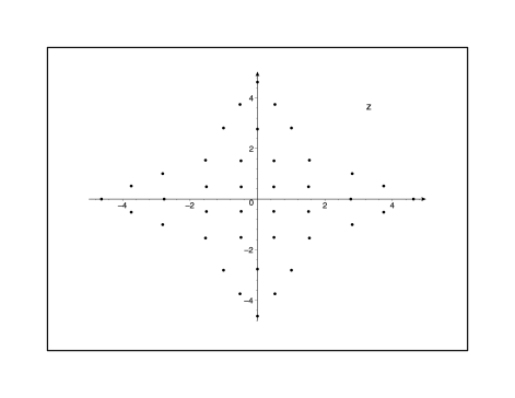
Figure 4: Configuration of zeros for the Okamoto polynomial $P_{4,4}(z)$

The configuration of zeros for the Okamoto polynomial $P_{4,4}(z)$ are demonstrated in the Figure 4.

7 Relations for the zeros of the generalized Hermite polynomials

Applying the transformation $y_{z}=w(z)y$ we get from (1.6) the following third-order differential equation

$$\begin{gathered}w_{{{zzz}}}+6\,{w_{{z}}}^{2}-4\,w_{{z}}{z}^{2}-8\,w_{{z}}\left(n-m\right)+4\,z\,w-8\,m\,n=0.\end{gathered}$$ (7.1)

The power expansion for its solutions near the point $z=z_{0}$ is

$$\begin{gathered}w(z)=\frac{1}{(z-{z_{0}})}+{a_{1}}+\frac{1}{3}\left({{z_{0}}}^{2}+2\,n-2\,m\right)\left(z-{z_{0}}\right)+\frac{1}{2}\,{z_{0}}\,{(z-z_{0})}^{2}+\\ \\ +\frac{4}{45}\left({{3}}-n{{z_{0}}}^{2}-{n}^{2}-mn+m{{z_{0}}}^{2}-{m}^{2}+\frac{3}{2}{z_{0}}{a_{1}}-\frac{1}{4}{{z_{0}}}^{4}\right)\left(z-{z_{0}}\right)^{3}+\\ \\ +\frac{1}{18}\left(2\,m{z_{0}}-{{z_{0}}}^{3}-2\,n{z_{0}}+3\,{a_{1}}\right)\left(z-{z_{0}}\right)^{4}+{a_{6}}\,\left(z-{z_{0}}\right)^{5}+...\end{gathered}$$ (7.2)

Using the series (7.2) we obtain the following relations for the zeros of the generalized Hermite polynomials

$$\begin{gathered}\sum_{k\neq j}^{nm}\frac{1}{(z_{k}-z_{j})}+a_{1}=0,\end{gathered}$$ (7.3)

$$\begin{gathered}\sum_{k\neq j}^{nm}\frac{1}{(z_{k}-z_{j})^{2}}+\frac{z_{j}^{2}}{3}+\frac{2\,(n-m)}{3}=0,\end{gathered}$$ (7.4)

$$\begin{gathered}\sum_{k\neq j}^{nm}\frac{1}{(z_{k}-z_{j})^{3}}+\frac{z_{j}}{2}=0,\end{gathered}$$ (7.5)

$$\begin{gathered}\sum_{k\neq j}^{nm}\frac{1}{(z_{k}-z_{j})^{4}}-\frac{z_{j}^{4}}{45}+\frac{4\,(m-n)z_{j}^{2}}{45}\,+\frac{2\,a_{1}\,z_{j}}{15}\,+\\ \\ +\frac{4}{45}\left({{3}}-{m}^{2}-m\,n-{n}^{2}\right)=0.\end{gathered}$$ (7.6)

The generalized Hermite polynomial $H_{4,4}(z)$ is [14]

$$\begin{gathered}H_{4,4}(z)={z}^{16}+15\,{z}^{12}-{\frac{225}{8}}\,{z}^{8}+{\frac{7875}{16}}\,{z}^{4}+{\frac{23625}{256}}.\end{gathered}$$ (7.7)

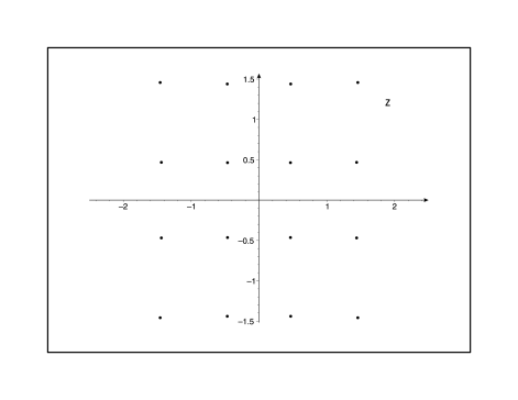
Figure 5: Configuration of zeros of the generalized Hermite polynomial $H_{4,4}(z)$

The configuration of the zeros of the generalized Hermite polynomial $H_{4,4}(z)$ are illustrated in the Figure 5.

8 Conclusion

In this work we have studied special polynomials associated with the rational solutions of the second, the third, and the fourth Painlevé equations. We have shown that if a family of polynomials satisfies an n-linear differential equation, then much information concerning the polynomials can be obtained from the asymptotic study of the solutions of a differential equation related to the original n-linear one. In particular, it can be found the degree of each polynomial, symmetric functions of its roots and some other correlations for the roots called the generalized Stieltjes relations. Also one can obtain possible degrees of the roots. In this work we have derived relations for the roots of the following polynomials: the Laguerre polynomials, the Umemura polynomials, the Ohyama polynomials, the generalized Okamoto polynomials, and the generalized Hermite polynomials. Our approach can be applied to other families of polynomials if there exists a differential equation satisfied by the family in question [28, 29, 30, 31].

9 Acknowledgments

This work was supported by the International Science and Technology Center under Project B 1213.

References

• [1] T. J. Stieltjes, Sur quelques theremes d’algebre, C.R. Acad. Sci.,Raris, 100 (1885) 439 - 440
• [2] T. J. Stieltjes, Sur les polynomials de Yacobi, C.R. Acad. Sci.,Raris, 100 (1885) 620 - 622
• [3] G. Szego, Ortogonal polynomials, vol. 23 (1959) New York, American Mathematical Society
• [4] A.P. Veselov, On Stieltjes relations, Painlevé -IV hierarchy and complex monodromy, J. Phys. A.: Math. Gen., 34 (2001) 3511 - 3519
• [5] F. Calogero, Equilibrium configuration of one - dimensional n - body problem with quadratic and inversely quadratic pair potentials, Lett. Nuovo Cimento, 20 (1977) 251 - 253
• [6] S. Ahmed, M. Bruschi, F. Calogero, M.A. Olshanetsky and FA.M. Perelomov, Properties of the zeros of the classical polynomials and of the bessel functions, Nuovo Cimento B, 49 (1979) 173 - 179
• [7] A.I. Yablonskii, On rational solutions of the second Painlevé equations, Vesti Akad. Nauk BSSR, Ser. Fiz. Tkh. Nauk, 3 (1959), 30 - 35 (in Russian)
• [8] A.P. Vorob’ev, On rational solutions of the second Painlevé equations, Differential equations 1 (1965) 79 - 81 (in Russian)
• [9] K. Okamoto, Studies on the Painlevé equations III, Math. Ann. 275 (1986) 221 - 255
• [10] H. Umemura, H. Watanabe, Solutions of the second and fourth Painlevé equations, I, Nagoya Math. J. Vol. 148 (1997) 151 - 198
• [11] P.A. Clarkson, Remarks on the Yablonskii - Vorob’ev Polynomials, Physics Letters A, 319, (2003) 137 - 144
• [12] P.A. Clarkson, On rational solutions of the fourth Painlevé Equation and its Hamiltonian (2004) CRM Proceedings and Lecture Notes, V. 39, (2004), 103 - 118
• [13] P.A. Clarkson, The third Painlevé equation and associated special polynomials, J. Phys. A: Math. Gen. (2003) 9507 - 9532
• [14] P.A. Clarkson, E.L. Mansfield, The second Painlevé equation, its hierarchy and associated special polynomials, Nonlinearity 16 (2003) R1
• [15] K. Iwasaki, H.Kimara, S. Shimomura, M. Yoshida, From Gauss to Painleve‘: A Modern Theory of Special Functions, 16 Aspects of Mathematics E, Vieweg, Braunschweig, Germany, 1991
• [16] T. Amdeberhan, Discriminants of Umemura polynomials associated to Painlevé III, Physics Letters A, 354 (2006), 410 - 413
• [17] M.V. Demina, N.A. Kudryashov, The Yablonskii - Vorob‘ev polynomials for the second Painlevé hierarchy, Chaos, Solitons and Fractals, v32(2),(2007), 526 - 537,
• [18] N.A. Kudryashov, M.V. Demina , Special polynomials associated with the fourth order analogue to the Painelvé equations, ArXiv SI/0605034, v.1, 16 May 2006
• [19] M.J.Ablowitz, P.A. Clarkson, Solitons, Nonlinear Evolution Equations and Inverse Scattering, Cambridge University press, Lecture Notes Series, 149,1991
• [20] R. Conte, The Painleve approach to Nonlinear Ordinary Differential equations, In ”The Painlevé property. One century later, CRM Series in Mathematical Physics”, Springer, (1999), New York, 177 - 180
• [21] N.A. Kudryashov, Analytical theory of nonlinear differential equations, Institute of Computer Investigations, Moscow-Izhevsk, (2004), 360 p. (in Russian)
• [22] F. Jrad, U. Mugan, Non - polynomial fourth order equations which pass the Painlevé test, Zeitschrift fur Naturforschung A, 60A (2005), 387 - 400
• [23] A.D. Bruno Power geometry in algebraic and differential equations, Moscow, Nauka, Fizmatlit, (1998), 288 p (in Russian)
• [24] A.D. Bruno, Asimptotics and expansions of solutions of ordinary differential equation, Uspehi Math. Nauk, 59 (3),(2004), 31-80 (in Russian)
• [25] A.D. Bruno, N.A. Kudryashov, Power expansions of solutions to analogy to the first Painlevé equation. Preprint of the Keldysh institute of Applied Mathematics of RAS, No. 17, Moscow, 2005 (in Russian)
• [26] M.V. Demina, N.A. Kudryashov, Power and non - power expansions of the solutions for the fourth - order analogue to the second Painlevé equation, Chaos, Solitons and Fractals, v. 32 (1),(2007), 124 - 144
• [27] N.A. Kudryashov, O.Yu. Efimova, Power expansions for solution of the fourth - order analog to the first Painlevé equation, Chaos, Solitons and Fractals, 30(1), (2006), 110-124
• [28] N.A. Kudryashov, The first Painlevé and the second Painlevé equations of higher order and some relations between them, Physics Letters A, v.224, (1997), 353 - 360
• [29] N.A. Kudryashov, Two hierarchies of ordinary differential equations and their properties, Phys. Lett. A 252 (1999) 173 - 179
• [30] Andrew N.W. Hone, Non - autonomous Henon - Heiles systems, Physica D 1998; 118: 1 - 16
• [31] C.M. Cosgrove, Higher - order Painlevé equations in the Polynomial class II: Bureau Symbol P1, Studies in Applied Mathematics, 116, (2006), 321 - 413