Synchronization processes in complex networks

Abstract

We present an extended analysis, based on the dynamics towards synchronization of a system of coupled oscillators, of the hierarchy of communities in complex networks. In the synchronization process, different structures corresponding to well defined communities of nodes appear in a hierarchical way. The analysis also provides a useful connection between synchronization dynamics, complex networks topology and spectral graph analysis.

, and

1 Introduction

In 1998 Watts and Strogatz presented a simple model of network’s structure that was the seed of the modern theory of complex networks [1]. Beginning with a regular lattice, they showed that the addition of a small number of random links reduces the diameter drastically. This effect, know as small-world effect, was detected in natural and artificial networks. The research was in part originally inspired by Watts’ efforts to understand the synchronization of cricket chirps, which show a high degree of coordination over long distances as though the insects where “invisibly” connected. Since then complex networks are being subject of attention of the physicists’ community [2, 3, 4, 5].

Complex networks are found in fields as diverse as the Internet, the World-Wide-Web, food-webs, and many forms of biological and social organizations (see [6] and references therein). The description of these networks, as it occurs in many physical systems, can be performed at different scales. At the lower level of description, the “microscale” is represented by single nodes. From the static point of view the key point is to determine certain properties of individual nodes (degree, centrality, clustering, etc.), while from the dynamics of the network point of view, the important issue is to know about the dynamical process each node is performing. This level of description is unfortunately very precise and does not allow a generic analysis of the global properties of the system. At the other extreme, we have the higher level of description, the “macroscale”, represented by the statistical properties of the network as a whole. This description has been the realm of statistical physics in complex networks and has provided great insight in the universality of certain features of many real world systems.

In the middle of these descriptions still remains a huge space for different scales of descriptions that we like to name as “mesoscales”, or intermediate scales. These scales are understood as substructures (eventually subgraphs) that have topological entity compared to the whole network, e.g. motifs [7, 8], cliques [9], cores [10], loops [11] or, generally speaking, communities [12]. In particular, the community detection problem concerning the determination of mesoscopic structures that have functional, relational or even social entity is still controversial, starting from the “a priori” definition of what a community is [14]. The correct determination of the mesoscale in complex networks is a major challenge. Under the name of the community detection problem, consisting in finding a ’good’ partition of the network in sub-graphs that represent communities according to a given definition, physicists have provided different methods that confront this challenge[13]. However, in many complex networks the organization of nodes is not completely represented by a unique partition but by a set of nested communities that appear at different topological scales. This evidence comes from indirect experimental data revealing functionalities in complex networks that involve different subsets of nodes at different hierarchical levels [15, 16].

In a completely different scenario, physicists have largely studied the dynamics of complex biological systems, and in particular the paradigmatic analysis of large populations of coupled oscillators [18, 19, 20]. The connection between the study of synchronization processes and complex networks is interesting by itself. Indeed, the original inspiration of Watts and Strogatz in the development of the Small-World network structure was, as mentioned before, to understand the synchronization of cricket chirps. This synchronization phenomena as many others e.g. asian fireflies flashing at unison, pacemaker cells in the heart oscillating in harmony, etc. have been mainly described under the mean field hypothesis that assumes that all oscillators behave identically and interact with the rest of the population. Recently, the emergence of synchronization phenomena in complex networks has been shown to be closely related to the underlying topology of interactions [17] beyond the macroscopic description.

In this paper we study of the dynamics towards synchronization in complex networks at the mesoscale description, extending previous results [21]. The paper is structured as follows: in section II we present the synchronization model studied. In section III we describe a method to construct synthetic networks with a well prescribed hierarchical community structure. In section IV, we expose the analysis of the route towards synchronization and their relationship with the topological structure. Finally, we conclude with a discussion about the synchronization processes in complex networks.

2 Synchronization: Kuramoto’s model

One of the most successful attempts to understand synchronization phenomena was due to Kuramoto [20], who analyzed a model of phase oscillators coupled through the sine of their phase differences. The model is rich enough to display a large variety of synchronization patterns and sufficiently flexible to be adapted to many different contexts [22]. The Kuramoto model consists of a population of $N$ coupled phase oscillators where the phase of the $i$-th unit, denoted by $\theta_{i}(t)$, evolves in time according to the following dynamics

$$\frac{d\theta_{i}}{dt}=\omega_{i}+\sum_{j}K_{ij}\sin(\theta_{j}-\theta_{i})\hskip 14.22636pti=1,...,N$$ (1)

where $\omega_{i}$ stands for its natural frequency and $K_{ij}$ describes the coupling between units. The original model studied by Kuramoto assumed mean-field interactions $K_{ij}=K,\forall i,j$. In absence of noise the long time properties of the population are determined by analyzing the only two factors which play a role in the dynamics: the strength of the coupling $K$ whose effect tends to synchronize the oscillators (same phase) versus the width of the distribution of natural frequencies, the source of disorder which drives them to stay away each other by running at different velocities. For unimodal distributions, there is a critical coupling $K_{c}$ above which synchronization emerges spontaneously.

Recently, due to the realization that many networks in nature have complex topologies, these studies have been extended to systems where the pattern of connections is local but not necessarily regular [23, 24, 25, 26, 27, 28, 29, 30, 31, 32]. Usually, due to the complexity of the analysis some further assumptions have been introduced. For instance, it has been a normal practice to assume that the oscillators are identical. Obviously, in absence of disorder, i.e. if $(\omega_{i}=\omega~{}\forall i)$ there is only one attractor of the dynamics: the fully synchronized regime where $\theta_{i}=\theta,~{}\forall i$. In this context the interest concerns not the final locked state in itself but the route to the attractor. In particular, it has been shown [33, 34] that high densely interconnected sets of oscillators (motifs) synchronize more easily that those with sparse connections. This scenario suggests that for a complex network with a non-trivial connectivity pattern, starting from random initial conditions, those highly interconnected units forming local clusters will synchronize first and then, in a sequential process, larger and larger spatial structures also will do it up to the final state where the whole population should have the same phase. We expect this process to occur at different time scales if a clear community structure exists. Thus, the dynamical route towards the global attractor will reveal different topological structures, presumably those which represent communities. Therefore, it is the complete dynamical process what unveils the whole organization at all scales, from the microscale at a very early stages up to the macroscale at the end of the time evolution. On the contrary, those systems endowed with a regular topological structure will usually display a trivial dynamics with a single time scale for synchronization, although some recent studies indicate also other possibilities [35].

It is a normal practice to define, for the Kuramoto model, a global order parameter to characterize the level of entrainment between oscillators. The normal choice is to use the following complex-valued order-parameter

$$re^{i\psi}=\frac{1}{N}\sum_{j=1}^{N}e^{i\theta_{j}}.$$ (2)

where $r(t)$ with $0\leq r(t)\leq 1$ measures the coherence of the oscillator population, and $\psi(t)$ is the average phase. However, this definition, although suitable for mean-field models is not efficient to identify local dynamic effects. In particular it does not give information about the route to the attractor (fully synchronization) in terms of local clusters which is so important to identify functional groups or communities. For this reason, instead of considering a global observable, we define a local order parameter measuring the average of the correlation between pairs of oscillators

$$\rho_{ij}(t)=<cos(\theta_{i}(t)-\theta_{j}(t))>$$ (3)

where the brackets stand for the average over initial random phases. The main advantage of this approach is that it allows to trace the time evolution of pairs of oscillators and therefore to identify compact clusters reminiscent of the existence of communities.

3 Structured complex networks

To give evidence of the aforementioned facts we have analyzed the dynamics towards synchronization –time evolution of $\rho_{ij}(t)$– in computer-generated graphs with community structure.

The paradigmatic model of network with a well defined community structure that has been used as a benchmark for different community detection algorithms [13], was proposed by Girvan and Newman [36]. In that model the authors construct a network of 128 nodes as a set of 4 communities, each one formed by 32 nodes. Fixing the mean number of links per node at a value of 16, the parameter describing the sharpness of the community distribution is $z_{in}$, the average number of links within the community. Here, we propose two generalizations of this model:

• Including communities of different sizes. In [37] it is shown that the algorithms for detecting the community structure are very sensitive to the size of the communities themselves, and a model to construct networks with inhomogeneous distributions of communities is proposed. In this case the networks are parametrized by two quantities, the internal and the external cohesion. As an example of such network see Fig.1a, with a clear distinction between the communities of different sizes.

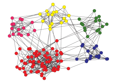
  a)	b)
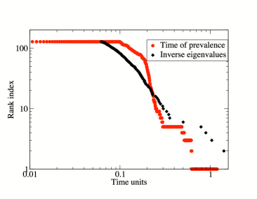
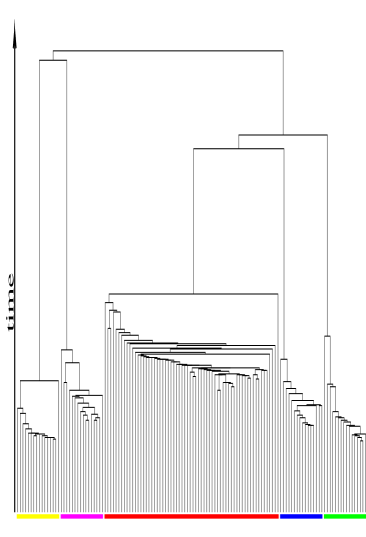
  c)	d)

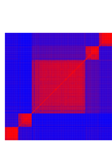
  Figure 1: Network with a inhomogeneous distribution of communities. a) the network structure; b) eigenvalues spectra and number of detected communities as a function of time; c) dendogram of the community merging. d) time needed for each pair of oscillators to synchronize. Red for shorter times, blue for larger times.

• Including several hierarchical levels of communities. We take a set of $N$ nodes and divide it into $n_{1}$ groups of equal size; each of these groups is then divided into $n_{2}$ groups and so on up to a number of steps $k$ which defines the number of hierarchical levels of the network. Then we add links to the networks in such a way that at each node we assign at random a number of $z_{1}$ neighbours within its group at the first level, $z_{2}$ neighbours within the group at the second level and so on. There is a remaining numbers of links that each node has to the rest of the network, that we will call $z_{out}$. In this case it is easy to compute the modularity of the partition [36] at any level $l\leq k$

  $$Q_{n_{1}\cdot n_{2}\cdot\ldots\cdot n_{l}}=\frac{z_{l}+\ldots+z_{k}}{z_{out}+z_{1}+\ldots+z_{k}}-\frac{1}{n_{1}\cdot n_{2}\ldots\cdot n_{l}}$$ (4)

  and its numerical value tells us how good as partition into a given community structure is. In [21] we considered networks with two hierarchical levels with 256 nodes, and $n_{1}=n_{2}=4$; this gives two possible partitions: one with 4 communities and the other one with 16 communities. In that case one can relate the more stable regions with larger values of modularity. Here we consider a network with 3 levels with 64 nodes for which $n_{1}=n_{2}=n_{3}=2$, see Fig.2a.

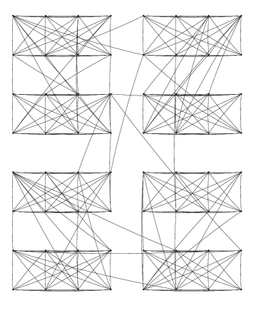
a)	b)
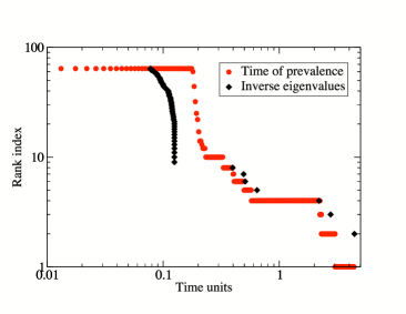
c)	d)

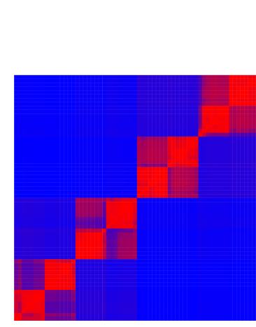
Figure 2: Network with 3 levels of communities. a) the network structure; b)eigenvalues spectra and number of detected communities as a function of time; c) dendogram of the community merging; d) time needed for each pair of oscillators to synchronize. Red for shorter times, blue for larger times.

In a different scenario, there is a set of deterministic networks that has been used as an example of hierarchical scale-free networks, proposed by Ravasz and Barabasi [38]. This type of networks, apart from its hierarchical structure has some nodes with a special role in terms of number of connexions (hubs) in contrast to the networks discussed previously that are essentially homogeneous in degree. In Fig. 3a we present a very simple example of this class of networks for the case of two hierarchical levels.

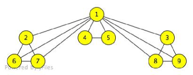
a)	b)
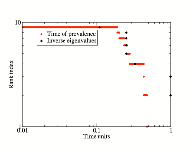
c)	d)

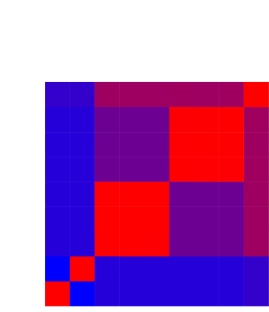
Figure 3: Deterministic network with 2 levels. a) the network structure; b) eigenvalues spectra and number of detected communities as a function of time; c) dendogram of the community merging; d) time needed for each pair of oscillators to synchronize. Red for shorter times, blue for larger times.

In a previous work [21] we represented the correlation matrix of the system $\rho_{ij}(t)$ at the same time instant $t$ for two slightly different two level hierarchical networks with structure 13-4 and 15-2. From that representation, we could identify the two levels of the hierarchical distribution of communities. The network 13-4 is very close to a state in which the four large groups are almost synchronized whereas the network 15-2 still presents some of the smaller groups of synchronized oscillators, and the larger group starting to synchronize, coherently with their topological structure. This picture that relates dynamics and topology, and distinguishes at a given time the two configurations, was our starting point and we follow this formalism in the next section.

4 The connection between synchronization and topology

The visualization of the correlation matrix of the system helps in elucidating the topology of the network. To extract the quantitative information it is useful to introduce some threshold $T$ to convert the correlation matrix into a binary matrix, that will be used to determine the borders between different groups. We define a dynamic connectivity matrix

$${\mathcal{D}}_{t}(T)_{ij}=\left\{\begin{array}[]{ll}1&\mbox{if }\rho_{ij}(t)>T\\ 0&\mbox{if }\rho_{ij}(t)<T\end{array}\right.$$ (5)

that depends on both the underlying topology and the collective dynamics. For a fixed time $t$, by moving the threshold $T$, we obtain different representations of ${\mathcal{D}}_{t}(T)$ that inform about the structure of the dynamic correlations. When the threshold is large enough the representation of ${\mathcal{D}}_{t}(T)$ becomes a set of disconnected clumps or communities. Decreasing $T$ a hierarchical structure of communities is devised. Note that since the function $\rho_{ij}(t)$ is continuous and monotonic (because the existence of a unique attractor of the dynamics), we can redefine ${\mathcal{D}}_{T}(t)$, i.e. fixing the threshold and evolving in time. We obtain the same information about the structure of the dynamic connectivity matrix at different time scales. These time scales unravel the topological structure of the connectivity matrix at different topological scales [21].

For instance, the eigenvalue spectrum of ${\mathcal{D}}_{T}(t)$, $S({\mathcal{D}}_{T}(t))$, can help in tracing the hierarchy of communities. In particular, the number of null eigenvalues corresponds to the number of connected components of the dynamical (synchronized) network. Thus, at short times, all units are uncorrelated and then we have $N$ disconnected sets, being $N$ the number of nodes in the network. As time goes on, nodes become synchronized in groups according to their topological structure. In panel b) of Figs. 1-3 we have plotted the number of non-connected components as a function of time for the three networks introduced in the previous section. At early stages the number of components is equal to the number of nodes whereas at final stages we have a single component. One of the remarkable results is the slope in these curves. Plateau regions indicate the relative stability of the dynamics at a given time scale whereas a vertical drop is related to instability. In [21] we already linked the stabililty of these regions with the eigenvalue spectrum of the Laplacian matrix, that we will investigate in detail later on.

Another interesting link between dynamics and topology, related with the discussion in the previous paragraph, comes from the analysis of the whole spectrum of the Laplacian matrix of the network graph ${\mathcal{L}}$ [40]. The Laplacian matrix is defined as ${\mathcal{L}}_{ij}=k_{i}\delta_{ij}-a_{ij}$, where $k_{i}$ is the degree of node $i$, $\delta_{ij}$ is the Kronecker delta and $a_{ij}$ is the element of the adjacency matrix (1 if nodes $i$ and $j$ are connected and 0 otherwise). The spectral information of the Laplacian matrix has been used to understand the structure of complex networks [41], and in particular to detect the community structure [42, 43] (also the spectral analysis of the modularity matrix [44] can be used to this end). Recent studies have also focused on the spectral information of the Laplacian matrix and the synchronization dynamics [23, 24, 25, 26, 27, 28, 29, 30]. The common approach is to take advantage of the master stability equation [45] to determine the relation between the relative stability of the synchronized state (via the ratio $\lambda_{N}/\lambda_{2}$) and the heterogeneity of the topology, although sometimes some language abuse appears and authors talk about better or worse synchonizability instead of stability of the synchronized state. Our approach differs from these works in the following: we are interested in the transient towards synchronization because it is this whole process which will reveal the topological structure at different scales. For this reason our analysis focus on the whole eigenvalue spectrum of the Laplacian matrix $S({\mathcal{L}})$. To characterize this spectrum, we rank the eigenvalues of ${\mathcal{L}}$ using an index $i$ in ascending order $0=\lambda_{1}\leq\lambda_{2}\leq\ldots\lambda_{i}\ldots\leq\lambda_{N}$. Panel b) of Figs. 1-3 shows the order of the eigenvalues in this ranking versus the inverse of its values, which closely corresponds to the time scales of emergence of nested communities of nodes. The structure of this sequence brings to light many aspects of the topological structure: (i) the number of null eigenvalues gives trivially the number of disconnected components of the static network, (ii) the gaps between consecutive eigenvalues tell us about the relative differences of time scales, and (iii) large eigenvalues in the last part of the series stands for the existence of hubs in the network (we will turn to these points later). In any case case the two curves on each of the panels b) show an intriguing similarity. The time scale related to a given eigenvalue corresponds roughly to the time scale at which a number of groups of oscillators are synchronized (which is shown by the number of connected components of the dynamical matrix).

In panel c) of Figs. 1-3 we have plotted the dendogram of the merging of the groups along the time evolution as it can be deduced from the time evolution of the correlation matrix. Groups merge as they get more correlated above some threshold (synchronized). We can clearly identify here the different topological scales, i.e. communities at different hierarchical levels.

Finally, in panel d) we plot the time that each pair of nodes need to synchronize. This picture complements the previous one, since it did not preserve the transitivity character of the merging. In the current picture transitivity plays no role and we can observe how pairs of nodes synchronize by itself and not by means of third parties.

5 Linear analysis

Finally we would like to shed some light about the intriguing relationship between the eigenvalues of the Laplacian and the dynamic structures that emerge in the route towards synchronization as shown in panel b) of Figs. 1-3. To understand this correspondence let us analyze the linearized dynamics of the Kuramoto model (i.e. the dynamics close to the attractor of synchronization) in terms of the Laplacian matrix,

$$\frac{d\theta_{i}}{dt}=-k\sum_{j}L_{ij}\theta_{j}\hskip 14.22636pti=1,...,N$$ (6)

whose solution in terms of the normal modes $\varphi_{i}(t)$ reads

$$\varphi_{i}(t)=\sum_{j}B_{ij}\theta_{j}=\varphi_{i}(0)e^{-\lambda_{i}t}\hskip 14.22636pti=1,...,N$$ (7)

where $\lambda_{i}$ are the eigenvalues of the Laplacian matrix, and $B$ is the matrix of eigenvectors. This set of equations has to be satisfied at any time $t$. If we rank the system of equations in descending order of the eigenvalues (i.e. starting from $\lambda_{N}$), the right hand side system of Eq.(7) will approach zero in a hierarchical way. This fact is equivalent in the dynamics to group oscillators surpassing the synchronization threshold forming communities. The gaps in the spectrum $S({\mathcal{L}})$ represent clearly different time scales between modes revealing different topological scales. The collective modes, solution of the system represented by Eq.(7), denote two types of behaviors. Some modes provide information about reorganization of the phases in the whole network, while the others inform about synchronization between pairs or groups of oscillators. The presence of hubs in the topology gives rise to large eigenvalues that decay very fast and are related to the first type of modes, those representing ”synchronization” between the hub and the topological average of the phases of rest of oscillators. The rest of modes relate oscillators that have similar projections on the corresponding eigenvectors thus giving rise to communities at a given topological scale. Indeed, this fact supports the success of the identification of communities using spectral analysis [42].

To illustrate these ideas we have explicitly analyzed two different types of networks: the star, which is a simple example of isotropic, homogeneous network without inner structure, and a simplified version of the Ravasz-Barabasi network, where we can easily identify all the time scales of the dynamic process and also to characterize and interpret the information provided by the spectrum of eigenvalues and eigenvectors of the laplacian matrix. The star consists of a network formed by two types of nodes: a hub, located in the middle of the network, connected to the rest of nodes and the peripherical nodes, not connected between them, only to the hub. It has been studied frequently in communication problems as a paradigm of system where all the traffic goes through a single node and therefore it is easy to collapse. The laplacian matrix of a n-node star (one hub and n-1 peripherical nodes) is

$$\left(\begin{array}[]{ccccc}-(n-1)&1&\cdots&1&1\\ 1&-1&\cdots&0&0\\ \vdots&\vdots&\vdots&\vdots&\vdots\\ 1&0&\cdots&-1&0\\ 1&0&\cdots&0&-1\\ \end{array}\right)$$ (8)

whose spectrum of eigenvectors has a very simple and compact structure:

$$(0,-1,\ldots,-1,-n)$$ (9)

two non-degenerate eigenvalues $(0,-n)$ and a $(n-2)$ times degenerate eigenvalue $(-1)$. The largest eigenvalue, in absolute value, gives information about the dynamical properties of the hub, while the smallest characterizes the attractor. To understand how the system of oscillators approaches the synchronized final state it is convenient to analyze the spectrum of eigenvectors in a hierarchical way starting again from the mode decaying first

$$\begin{array}[]{ccccc}\lambda=-n&&v_{1}&=&(-(n-1),1,1,1,\ldots,1,1,1)\\ \lambda=-1&&v_{2}&=&(0,-1,1,0,\ldots,0,0)\\ \lambda=-1&&v_{3}&=&(0,-1,0,1,\ldots,0,0)\\ \vdots&&\ldots\\ \lambda=-1&&v_{(n-1)}&=&(0,-1,0,\ldots,0,0,1)\\ \lambda=0&&v_{n}&=&(1,1,1,1\ldots,1,1,1)\end{array}$$ (10)

The dynamical evolution of the system can be interpreted as follows. The equation related to the largest eigenvalue reads

$$\sum_{j}B_{1j}\theta_{j}=e^{-nt}$$ (11)

It means that in a first stage, almost instantaneously, the phase of the hub goes to

$$\theta_{1}=\frac{1}{n-1}\sum_{i>1}\theta_{i}$$ (12)

that is an arithmetic average over the peripherical units. In a second stage, the rest of phases synchronize in pairs $\theta_{i}=\theta_{j}\hskip 4.30554pt\forall i,j\neq 1$. Therefore, we can identify two different types of collective modes, one tending to reorganize the phases of some units while the rest describe the physical entrainment between oscillators. Notice that the synchronization process takes place in a single time scale which is reflected in the spectral properties of the laplacian matrix as the set of eigenvalues is multiply degenerate.

A more complex situation is presented in the simplified Ravasz-Barabasi network Fig.3a. In contrast to the uniform structure of the star, this network displays an internal topological structure in two levels. Therefore, we expect a rich dynamical evolution which also should be reflected in the spectrum of eigenvalues of the laplacian matrix. Now, the laplacian matrix reads

$$\left(\begin{array}[]{ccccccccc}-8&1&1&1&1&1&1&1&1\\ 1&-3&0&0&0&1&1&0&0\\ 1&0&-3&0&0&0&0&1&1\\ 1&0&0&-2&1&0&0&0&0\\ 1&0&0&1&-2&0&0&0&0\\ 1&1&0&0&0&-3&1&0&0\\ 1&1&0&0&0&1&-3&0&0\\ 1&0&1&0&0&0&0&-3&1\\ 1&0&1&0&0&0&0&1&-3\\ \end{array}\right)$$ (13)

whose spectrum of eigenvalues and eigenvectors is

$$\begin{array}[]{ccccc}\lambda=-9&&v_{1}&=&(-8,1,1,1,1,1,1,1,1)\\ \lambda=-4&&v_{2}&=&(0,0,-1,0,0,0,0,1,0)\\ \lambda=-4&&v_{3}&=&(0,0,-1,0,0,0,0,0,1)\\ \lambda=-4&&v_{4}&=&(0,-1,0,0,0,1,0,0,0)\\ \lambda=-4&&v_{5}&=&(0,-1,0,0,0,0,1,0,0)\\ \lambda=-3&&v_{6}&=&(0,0,0,-1,1,0,0,0,0)\\ \lambda=-1&&v_{7}&=&(0,1,0,\frac{-3}{2},\frac{-3}{2},1,1,0,0)\\ \lambda=-1&&v_{8}&=&(0,0,1,\frac{-3}{2},\frac{-3}{2},0,0,1,1)\\ \lambda=0&&v_{9}&=&(1,1,1,1,1,1,1,1,1)\end{array}$$ (14)

The analysis of the dynamical relaxation of the eigenmodes shows the following aspects. First, a reorganization process takes place involving the phases of the hub with the rest of oscillators. This stage is similar to that observed in the star because the hub is again is a fully connected unit. The four-fold degenerate eigenvalue $\lambda=-4$ describes the entrainment process between 6 nodes. This behavior is quite appealing because although they are not directly connected they are topologically equivalent and belong to the same structural level. These results show that one has to consider other elements more important than physical connectivity when defining the concept of community in complex networks. Later, at a slightly larger time scale units 4 and 5 synchronize. Finally these nodes synchronize with the two equivalent functional groups as can be stated from the two modes associated to the eigenvalue $\lambda=-1$. The results are in perfect agreement with the synchronization times of the full non-linear dynamics as we can see in the dendrogram of Fig. 3.

In general, as a rule of thumb, those networks whose structure is random and where all the nodes play the same statistical role from a topological standpoint are characterized by a continuum spectrum of eigenvalues. In contrast, when the network has a specific internal structure, which for social or biological networks might be the fingerprint of different functional groups, then we expect a Laplacian spectrum with different gaps stressing the existence of different time scales in the dynamic process towards the attractor.

6 Summary

We have analyzed the synchronization dynamics in complex networks and show how this process unravels its different topological scales. We have also reported a connection between the spectral information of the Laplacian matrix and the hierarchical process of emergence of communities at different time scales. We show for a set of structured networks that the gaps in the spectrum are related to the stability of the hierarchical structures (communities) of the networks. We propose additional graphical tools to understand how the synchronization process takes place: a dendogram of the merging of the synchronized groups and a visualtization of the time needed for each pair of oscillators to synchronize.

References

- [1] D. J. Watts, S. H. Strogatz, Nature 393, 440 (1998).
- [2] S. Strogatz, Nature 410, 268 (2001).
- [3] R. Albert and A.-L. Barabasi, Rev. Mod. Phys. 74, 47 (2002).
- [4] M. E. J. Newman, SIAM Review 45, 167 (2003).
- [5] S. Boccaletti, V. Latora, Y. Moreno, M. Chavez, and D.-U. Hwang, Phys. Rep. 424, 175 (2006).
- [6] M. Buchanan, Nexus (W.W. Norton NewYork - London, 2002).
- [7] R Milo, S Shen-Orr, S Itzkovitz, N Kashtan, D. Chklovskii and U. Alon, Science 298, 824 (2002).
- [8] N. Kashtan and U. Alon, PNAS 102, 13773 (2005).
- [9] G. Palla, I. Derenyi, I. Farkas and V. Tamas, Nature 435, 814 (2005)
- [10] S. Wuchty and E. Almaas, BMC Evol. Biol. 5, 24 (2005).
- [11] G. Bianconi and A. Capocci, Phys. Rev. Lett. 90, 078701 (2003)
- [12] M. E. J. Newman, Eur. Phys. J. B 38, 321 (2004).
- [13] L. Danon, A. Diaz-Guilera, J. Duch, and A. Arenas, J. Stat. Mech. P09008 (2005).
- [14] S. Wasserman and K. Faust. Social Network Analysis (Cambridge University Press, New York, 1994).
- [15] E. Ravasz, A. L. Somera, D. A. Mongru, Z. N. Oltvai, A.-L. Barab si, Science 297, 1551 (2002).
- [16] A. W. Rives and T. Galitski, PNAS 100, 1128 (2003).
- [17] F. M. Atay, T. Biyikoglu, and J. Jost. IEEE Trans. Circuits and Systems 53, 92 (2006).
- [18] A. T. Winfree, The geometry of biological time (2nd ed. Springer-Verlag, 2001).
- [19] S. H. Strogatz, Sync: The Emerging Science of Spontaneous Order (New York: Hyperion, 2003).
- [20] Y. Kuramoto, Chemical oscillations, waves, and turbulence (2nd ed. Mineola NY, Dover Publications, 2003).
- [21] A. Arenas, A. Diaz-Guilera and C.J. Perez-Vicente, Phys. Rev. Lett. 96, 114102, (2006).
- [22] J. A. Acebron, L. L. Bonilla, C. J. Perez Vicente, F. Ritort, and R. Spigler, Rev. Mod. Phys. 77,137 (2005).
- [23] M. Barahona and L. M. Pecora, Phys. Rev. Lett. 89, 054101 (2002).
- [24] T. Nishikawa, A.E. Motter, Y.-C. Lai, and F.C. Hoppensteadt, Phys. Rev. Lett. 91, 014101 (2003).
- [25] Y. Moreno and A. F. Pacheco, Europhys. Lett. 68, 603, (2004).
- [26] H. Hong, B. J. Kim, M.Y. Choi, and H. Park, Phys. Rev. E 69, 067105 (2004).
- [27] A.E. Motter, C. Zhou, and J. Kurths, Phys. Rev. E 71, 016116 (2005).
- [28] D.-S. Lee, Phys. Rev. E 72, 026208 (2005).
- [29] L. Donetti, P. I. Hurtado, and M. A. Muñoz, Phys. Rev. Lett. 95, 188701 (2005).
- [30] M. Chavez, D.-U. Hwang, A. Amann, H. G. E. Hentschel, and S. Boccaletti, Phys. Rev. Lett. 94, 218701 (2005).
- [31] J. G. Restrepo, E. Ott, and B. R. Hunt, Phys. Rev. E 71, 036151 (2005).
- [32] J. G. Restrepo, E. Ott, and B. R. Hunt, Chaos 16, 015107 (2006).
- [33] Y. Moreno, M. Vazquez-Prada, and A. F. Pacheco, Physica A, 343, 279 (2004).
- [34] E. Oh, K. Rho, H. Hong, and B. Kahng, Phys. Rev. E 72, 047101 (2005).
- [35] D. A. Wiley, S.H. Strogatz, and M. Girvan, Chaos 16(1), 015103 (2006).
- [36] M. E. J. Newman and M. Girvan, Phys. Rev. E 69, 026113 (2004).
- [37] L. Danon, A. Díaz-Guilera and A. Arenas, preprint physics/0601144 (2006).
- [38] E. Ravasz and A.-L. Barabasi, Phys. Rev. E 67, 026112 (2003).
- [39] We prescribe the value of the threshold to 0.999. Other choices do not alter the results, since it only modifies the relative time scales.
- [40] N.L. Biggs, Algebraic Graph Theory, Cambridge University Press (1974).
- [41] I. J. Farkas, I. Derenyi, A.-L. Barabasi, and T. Vicsek, Phys. Rev. E 64, 026704 (2001).
- [42] L. Donetti and M. A. Muñoz, J. Stat. Mech. P10012 (2004).
- [43] A. Capocci, V. D. P. Servedio, G. Caldarelli, and F. Colaiori, Physica A 352 669 (2005).
- [44] M. E. J. Newman, Proc. Natl. Acad. Sci. USA 103, 8577 (2006).
- [45] L. M. Pecora and T. L. Carroll, Phys. Rev. Lett. 80, 2109 (1998).