Energy Conservation and Second-Order Statistics
in Stably Stratified Turbulent Boundary Layers

Abstract

We address the dynamical and statistical description of stably stratified turbulent boundary layers with the important example of the atmospheric boundary layer with a stable temperature stratification in mind. Traditional approaches to this problem, based on the profiles of mean quantities, velocity second-order correlations, and dimensional estimates of the turbulent thermal flux run into a well known difficulty, predicting the suppression of turbulence at a small critical value of the Richardson number, in contradiction with observations. Phenomenological attempts to overcome this problem suffer from various theoretical inconsistencies. Here we present an approach taking into full account all the second-order statistics, which allows us to respect the conservation of total mechanical energy. The analysis culminates in an analytic solution of the profiles of all mean quantities and all second-order correlations removing the unphysical predictions of previous theories. We propose that the approach taken here is sufficient to describe the lower parts of the atmospheric boundary layer, as long as the Richardson number does not exceed an order of unity. For much higher Richardson numbers the physics may change qualitatively, requiring careful consideration of the potential Kelvin-Helmoholtz waves and their interaction with the vortical turbulence.

Nomenclature 
 
$\bm{\mathcal{A}}$ Thermal flux production vector, (I.1) $\beta$ Buoyancy parameter, ${\bm{g}}\widetilde{\beta}$ $\bm{\mathcal{B}}$ Pressure-temperature-gradient-vector, (12f) $\widetilde{\beta}$ Thermal expansion coefficient, (47d) ${\mathcal{C}}_{ij}$ Energy conversion tensor, (12b) $\gamma_{\scriptscriptstyle\rm{RI}}$ Relaxation frequency of $\tau_{ij}$, $i=j$ ${\mathcal{D}}/{\mathcal{D}}t$ Substantial derivative, $\partial/\partial t+\bm{\mathcal{U}}\!\cdot\!{\bm{\nabla}}$ $\widetilde{\gamma}_{\scriptscriptstyle\rm{RI}}$ Relaxation frequency of $\tau_{ij}$, $i\neq j$ $D/Dt$ Mean substantial derivative, $\partial/\partial t+{\bm{U}}\!\cdot\!{\bm{\nabla}}$ $\gamma_{\scriptscriptstyle\rm{RD}}$ Relaxation frequency of ${\bm{F}}$ $E_{\scriptscriptstyle\rm{K}}$ Turbulent kinetic energy per unit mass, $\frac{1}{2}|{\bm{u}}|^{2}$ $\gamma_{uu}$ Relaxation frequency of $E_{\scriptscriptstyle\rm{K}}$ $E_{\scriptscriptstyle\rm{\Theta}}$ ”Temperature energy” per unit mass, $\frac{1}{2}\theta^{2}$ $\gamma_{\theta\theta}$ Relaxation frequency of $E_{\scriptscriptstyle\rm{\Theta}}$ ${\bm{F}}$ Turbulent thermal flux per unit mass, $\left\langle{\bm{u}}\theta\right\rangle$ $\varepsilon_{ij}$ Dissipation tensor of $\tau_{ij}$, (11) $F_{*}$ Thermal flux at zero elevation $z=0$ ${\bm{\epsilon}}$ Dissipation vector of ${\bm{F}}$, (11) ${\bm{g}}$ Gravity acceleration, ${\bm{g}}=-g\,\widehat{\bf{z}}$ $\varepsilon$ Dissipation of $E_{\scriptscriptstyle\rm{\Theta}}$, (11) $L$ Monin-Obukhov length, $u_{*}^{3}/\beta F_{*}$ $\Theta$ Total potential temperature $\ell$ Outer scale of turbulence, external parameter $\Theta_{d}$ Deviation of $\Theta$ from BRS ${\mathcal{P}}_{ij}$ Rate of Reynolds stress production, (12a) $\overline{\Theta}$ Mean potential temperature, $\left\langle\Theta_{d}\right\rangle$ $p$, $\widetilde{p}$, $p_{*}$ Total, fluctuating and zero level pressures $\theta$ Fluctuating potential temperature Pr_T Turbulent Prandtl number, $\nu_{\scriptscriptstyle\rm{T}}/\chi_{\scriptscriptstyle\rm{T}}$ $\theta_{*}$ Potential temperature Ri_flux Flux Richardson number, $\beta F_{z}/\tau_{xz}S_{\scriptscriptstyle\rm{U}}$ at zero elevation, $F_{*}/u_{*}$ Ri_grad Gradient Richardson number, $\beta S_{\scriptscriptstyle\rm{\Theta}}/S^{2}_{\scriptscriptstyle\rm{U}}$ $\lambda_{*}$ Viscous lengthscale, $\nu/u_{*}$ ${\mathcal{R}}_{ij}$ Pressure-rate-of-strain-tensor, (12c) $\nu$ Kinematic viscosity $S_{\scriptscriptstyle\rm{U}}$ Mean velocity gradient, $dU/dz$ $\nu_{\scriptscriptstyle\rm{T}}$ Turbulent viscosity $S_{\scriptscriptstyle\rm{\Theta}}$ Mean potential temperature gradient, $d\overline{\Theta}/dz$ $\rho$ density of the fluid $T$ Molecular temperature $\tau_{ij}$ Reynolds stress tensor, $\left\langle u_{i}u_{j}\right\rangle$ $\bm{\mathcal{U}}$ Velocity field $\tau_{*}$ Mechanical momentum flux ${\bm{U}}$ Mean velocity, $\left\langle\bm{\mathcal{U}}\right\rangle$ at zero elevation (at the graund) ${\bm{u}}$ Fluctuating velocity, $\bm{\mathcal{U}}-{\bm{U}}$ $\chi$ dynamical thermal conductivity $u_{*}$ (Wall) friction velocity, $\sqrt{\tau_{*}}$ $\chi_{\scriptscriptstyle\rm{T}}$ Turbulent thermal conductivity $\widehat{\bf{x}}$, $\widehat{\bf{z}}$ stream-vise and vertical (wall-normal) directions BRS Basic Reference State
 

Introduction

The lower levels of the atmosphere are usually strongly influenced by the Earth’s surface. Known as the atmospheric boundary layer, this is the part of the atmosphere where the surface influences the temperature, moisture, and velocity of the air above through the turbulent transfer of mass.

The stability of the atmospheric boundary layer depends on the profiles of the density and the temperature as a function of the height above the ground. During normal summer days the land mass warms up and the temperature is higher at lower elevations. If it were not for the decrease in density of the air as a function of the height, such a situation of heating from below would have been always highly unstable. In fact, the boundary layer is considered stable as long as the temperature decreases at the dry adiabatic lapse rate ($T^{\prime}\approx-9.8^{\circ}C$ per kilometer) throughout most of the boundary layer. With such a rate of cooling one balances out the decrease in density. With a higher degree of cooling one refers to the atmospheric boundary layer as unstably stratified, whereas with a lower degree of cooling the situation is stably stratified. Stably stratified boundary layer occurs typically during clear, calm nights. In extreme cases turbulence tends to cease, and radiational cooling from the surface results in a temperature that increases with height above the surface.

The tendency of the atmosphere to be turbulent does not depend only on the rate of cooling but also on the mean shear in the vertical direction. The commonly used parameter to describe the tendency of the atmosphere to be turbulent is the “gradient” Richardson number (Richardson, 1920), defined as

$$\mbox{Ri}_{\rm{grad}}\equiv\frac{\beta\,d\Theta(z)\big{/}dz}{[dU_{x}/dz]^{2}}\,,$$ (1)

where $x$ is the stream-wise direction, $z$ is the height above the ground, $\overline{\Theta}(z)$ is the the “mean potential temperature” profile, (which differs from the mean temperature profile $T(z)$ by accounting for the adiabatic cooling of the air during its expansion: $d\overline{\Theta}(z)\big{/}dz=dT(z)\big{/}dz+|T^{\prime}|$), $\beta=\widetilde{\beta}g$ is the buoyancy parameter in which $\tilde{\beta}$ is the adiabatic thermal expansion coefficient, [defined below in Eq. (47d); for an ideal gas $\widetilde{\beta}=1/T$], and $g$ is the gravitational acceleration. The mean shear $dU_{x}/dz$ is defined in terms of the mean velocity ${\bm{U}}$, which in the simplest case of flat geometry depends only on the vertical coordinate $z$. The parameter $\mbox{Ri}_{\rm{grad}}$ represents the ratio of the generation or suppression of turbulence by buoyant production of energy to the mechanical generation of energy by wind shear.

In this paper we consider the description of stably stratified turbulent boundary layers (TBL), taking as an example the case of stable thermal stratification. Since the 50’s of twentieth century, traditional models of stratified TBL generalize models of unstratified TBL, based on the budget equations for the kinetic energy and mechanical momentum; see reviews of Umlauf and Burchard (2005), Weng and Taylor (2003). The main difficulty is that the budget equations are not closed; they involve turbulent fluxes of mechanical moments $\tau_{ij}$ (known as the “Reynolds stress” tensor) and a thermal flux ${\bm{F}}$ (for the case of thermal stratification):

$$\tau_{ij}\equiv\langle u_{i}u_{j}\rangle\,,\quad{\bm{F}}\equiv\left\langle{\bm{u}}\,\theta\right\rangle\,,$$ (2)

where ${\bm{u}}$ and $\theta$ stand for the turbulent fluctuating velocity and the potential temperature with zero mean. The nature of the averaging procedure behind the symbol $\langle\cdots\rangle$ will be specified below.

Earlier estimates of the fluxes (2) are based on the concept of the down-gradient turbulent transport, in which, similarly to the case of molecular transport, the flux is taken proportional to the gradient of transported property times a corresponding (turbulent) transport coefficient:

$$\tau_{xz} = -\nu_{\scriptscriptstyle\rm{T}}{dU_{x}}\big{/}{dz}\,,\quad\nu_{\scriptscriptstyle\rm{T}}\approx C_{\nu}\,\ell_{z}\sqrt{\tau_{zz}}\,,$$ (3a)

$$F_{z} = -\chi_{\scriptscriptstyle\rm{T}}{d\Theta}\big{/}{dz}\,,\quad~{}\chi_{\scriptscriptstyle\rm{T}}\approx C_{\chi}\,\ell_{z}\sqrt{\tau_{zz}}\,,\quad\mbox{etc.}~{}~{}~{}~{}$$ (3b)

Here the turbulent-eddy viscosity $\nu_{\scriptscriptstyle\rm{T}}$ and turbulent thermal conductivity $\chi_{\scriptscriptstyle\rm{T}}$ are estimated by dimensional reasoning via the vertical turbulent velocity $\sqrt{\tau_{zz}}$ and a scale $\ell_{z}$ (which in the simplest case is determined by the elevation $z$). The dimensionless coefficients $C_{\nu}$ and $C_{\chi}$ are assumed to be of the order of unity.

This approach meets serious difficulties (Zeman, 1981), in particular, it predicts a full suppression of turbulence when the stratification exceeds a critical level, for which $\mbox{Ri}_{\rm{grad}}=$Ri${}_{\rm{cr}}\approx 0.25$. On the other hand, in observations of the atmospheric turbulent boundary layer turbulence exists for much larger values than $\mbox{Ri}_{\rm{grad}}=0.25$: experimentally above $\mbox{Ri}_{\rm{grad}}=10$ and even more (for detailed discussion see Zilitinkevich et al., submitted to Science). In models for weather predictions this problem is “fixed” by introducing fit functions $C_{\nu}(\mbox{Ri}_{\rm{grad}})$ and $C_{\chi}(\mbox{Ri}_{\rm{grad}})$ instead of the constant $C_{\nu}$ and $C_{\chi}$ in the model parametrization (3). This technical “solution” is not based on a physical derivation and just masks the shortcomings of the model. To really solve the problem one has to understand its physical origin, even though from a purely formal viewpoint it is indeed possible that a dimensionless coefficient like $C_{\chi}$ can be any function of $\mbox{Ri}_{\rm{grad}}$.

To expose the physical reason for the failure of the down-gradient approach, recall that in a stratified flow, in the presence of gravity, the turbulent kinetic energy is not an integral of motion. Only the total mechanical energy, the sum of the kinetic and the potential energy, is conserved in the inviscid limit. As it was shown already by Richardson, the difficult point is that an important contribution to the potential energy comes not just from the mean density profile, but from the density fluctuations. Clearly, any reasonable model of the turbulent boundary layer must obey the conservations laws.

The physical requirement of conserving the total mechanical energy calls for an explicit consideration not only of the mean profiles, but also of all the relevant second-order, one-point, simultaneous correlation functions of all the fluctuating fields together with some closure procedure for the appearing third order moments. First of all, in order to account for the important effect of stratification on the anisotropy, we must write explicit equations for the entire Reynolds stress tensor, $\tau_{ij}=\left\langle u_{i}u_{j}\right\rangle$ . Next, in the case of the temperature stratified turbulent boundary layers we follow tradition [see, e.g. see e.g. Zeeman, (1981), Hunt et al. (1988), Schumann and Gerz (1995), Hanazaki and Hunt (2004), Keller and van Atta (2000), Stretch et al. (2001), Elperin et al. (2002), Cheng et al. (2002) Luyten et al. (2002), and Rehmann and Hwang (2005)] and account for the turbulent potential energy which is proportional to the variance of the potential temperature deviation, $\langle\theta^{2}\rangle$. And last but not least, we have to consider explicitly equations for the the vertical fluxes, $\tau_{xz}$ and $F_{z}$, which include the down gradient terms proportional to the velocity and temperature gradients, and counter-gradient terms, proportional to $F_{x}$ (in the equation for $\tau_{xz}$) and to $\left\langle\theta^{2}\right\rangle$ (in the equation for $F_{z}$) .

Unfortunately, the resulting second order closure seems to be inconsistent with the variety of boundary-layer data, and many authors took the liberty to introduce additional fitting parameters and sometimes fitting functions to achieve a better agreement with the data (see reviews of Umlauf and Burchard (2005), Weng and Taylor (2003), Zeeman, (1981), Melor and Yamada (1974), and references therein). Moreover, in the second order closures the problem of critical Richardson number, Ri_cr, seems to persists (Cheng et al., 2002; Canuto, 2002).

An interesting attempt to improve the modeling of stably stratified flows with the aim to remove Ri_cr is reported in a paper by Zilitinkevich, Elperin, Kleeorin and Rogachevskii (2007) in this issue, referred hereafter to as the ZEKR-paper. Following the traditional second-order scheme (see e.g. Zeeman, 1981), they removed the unwarranted approximation (3b), and replace it with an exact equation for the vertical thermal flux $F_{z}$ and for the “temperature energy” $\left\langle\theta^{2}\right\rangle/2$, using dimensional reasoning to estimate required third-order correlations. To account for the important effect of stratification on the anisotropy of turbulence, they, in agreement with Cheng et al. (2002), explicitly considered budget equations for the partial kinetic energies $\tau_{ii}/2$. Nevertheless ZEKR do not close rigorously the momentum budget equation. They combine three terms in this equations into, what they called “effective dissipation rate”, arriving actually again at the down-gradient approximation (3a) for the vertical flux of $x$-component of the mechanical moment, $\tau_{xz}$. In our paper we treat these three terms separately, considered also explicitly the horizontal heat flux $F_{x}$.

Notice that in spite of obvious inconsistency of the first-order schemes, “most of the practically used turbulent models are based on the concept of the down-gradient transport”. One of the reasons is that in the second-order schemes instead of two down-gradient equations (3) one needs to take into account eight nonlinear coupled additional equations i.e. four equations for the Reynolds stresses, three equations for the heat fluxes and equation for the temperature variance. As the result, second-order schemes have seemed to be rather cumbersome for comprehensive analytical treatment and have allowed to find only some relationships between correlation functions (see, e.g., Cheng et al., 2002). Unfortunately, the numerical solutions to the complete set of the second-order schemes equations which involve too many fitting parameters are much less informative in clarification of physical picture of the phenomenon than desired analytical ones.

In this paper we suggest a relatively simple second-order closure model of turbulent boundary layer with stable temperature stratification that, from the one hand, accounts (as we believe) for main relevant physics in the stratified TBL and, from the other hand, is simple enough to allow complete analytical treatment including the problem of critical Ri_grad. To reach this goal we approximate the third order correlations via the first- and second-order ones, accounting only for the most physically important terms. We will try to expose the approximations in a clear and logical way, providing the physical justification as we go along. Resulting second-order model consist of nine coupled equations for the mean velocity and temperature gradients, four components of the Reynolds stresses, two components of the temperature fluxes and the temperature variance. Thanks to the achieved simplicity of the model we found an approximate analytical solution of these equations, expressing all nine correlations as functions of only one governing parameter, $\ell(z)/L$, where $\ell(z)$ is the outer scale of turbulence (depending on the elevation $z$ and also known as the “dissipation scale”) and $L$ – is the Monin-Obuckhov length.

We would like also to stress, that in our approach $\ell(z)/L$ is an external parameter of the problem. For small elevations $z\ll L$, it is well accepted that $\ell(z)$ is proportional to $z$, while the $\ell(z)$ dependence is still under debate for $z$ comparable or exceeding $L$. For $z\gtrsim L$ the assignment and discussion of the actual dependence of the outer scale of turbulence, $\ell(z)$, which is manifested in the nature is out of the scope of this paper, and is remained for future work. At time being, we can analyze consequences of our approach for the following versions of $\ell(z)$ dependence at $z\gg L$:
•  function $\ell(z)$ is saturated at some level of the order of $L$. For concreteness we can take

$$1/\ell(z)=\sqrt{(d_{1}z)^{-2}+(d_{2}L)^{-2}}\,,\quad d_{1}\sim d_{2}\sim 1\ .$$ (4)

•  $\ell(z)$ is again proportional to $z$ for elevations much larger than $L$: $\ell(z)=d_{3}z$ but with the proportionality constant $d_{3}<d_{1}$. If so, we can also study the case $\ell(z)\gg L$ even though such a condition may not be realizable in nature. In that case our analysis of the limit $\ell(z)\gg L$ has only a methodological character: it allows to derive an approximate analytic solution for all the objects of interest as functions of $\ell(z)/L$ that, of course, is also valid for the outer scale of turbulence not exceeding a value of the order of $L$.

It should be noticed that traditional turbulent closures (including ours) cannot be applied for strongly stratified flows with $\mbox{Ri}_{\rm{grad}}\gtrsim 1$ (may be even at $\mbox{Ri}_{\rm{grad}}\sim 1$). The main reason is that these closures are roughly justified for developed vortical turbulence, in which the eddy-turnover time is of the order of its life time; in other words, there are no well defined “quasi-particles” or waves. This is NOT the case for stable stratification with $\mbox{Ri}_{\rm{grad}}\gtrsim 1$, in which the Brunt-Väisälä frequency

$$N\equiv\sqrt{\beta d\Theta(z)/d\,z}\,,$$ (5)

is larger then the eddy-turnover frequency $\gamma$. It means that for $\mbox{Ri}_{\rm{grad}}\gtrsim 1$ there are weakly decaying Kelvin-Helmholts internal gravity waves (with characteristic frequency $N$ and decay time above $1/\gamma$), propagating on large distances, essentially effecting on TBL, as pointed out by Zilitinkevich, (2002). In contrast to ambitious ZEKR attempt to describe entire TBL without limitation in values of $\mbox{Ri}_{\rm{grad}}$, and without explicit accounting for the internal gravity waves, we concentrate in our paper on self-consistent description of the lower part of the atmospheric TBL, in which turbulence has vortical character and consequently, large values of $\mbox{Ri}_{\rm{grad}}$ do not appear. We relate large values of $\mbox{Ri}_{\rm{grad}}$ in the upper part of TBL with contributions of the internal gravity waves to the energy and the energy flux in TBL, to the momentum flux, and to the production of (vortical) turbulent energy. Due to their instability in a shear flow, the waves can break and create turbulent kinetic energy. All these effects are beyond the framework of our paper. Their description in the upper “potential-wave” TBL and intermediate region with the combined “vortical-potential” turbulent velocity field is in our nearest agenda.

To make the paper more transparent for wide audience, not necessarily experts in atmospheric TBL, we attempt to present the material in a self-contained manner, and organized it as follows.

In Sect. IA we used the Oberbeck-Boussinesq approximation and applied the standard Reynolds decomposition (into mean values and turbulent zero-mean fluctuations of the velocity and temperature fields) to derive equations for the mean values and balance equations for all the relevant second-order correlation functions. In Sect. IB we demonstrate that the resulting balance equations exactly preserve (in the non-dissipative limit) the total mechanical energy of the system, that consists of the kinetic energy of the mean flow, kinetic energy and potential energy of the turbulent subsystem.

In Sect. II we describe the proposed closure procedure that results in a model of stably stratified TBL, that accounts explicitly for all the relevant second-order correlations. The third order correlations which appear in the theory are modeled in terms of second-order correlations in Sects. IIA and B. Further simplifications are presented in Sects. IIC and D for stationary turbulent flows in a plane geometry outside the viscous and buffer layers. In Sect. IIE we suggest some generalization of the standard “wall-normalization” to obtain the model equations in dimensionless form with only one governing parameter, $\ell(z)/L$.

Section III.1 contains approximate analytical solution of the model. It is shown that the analytical solution deviates from the numerical counterpart in less than a few percent in the entire interval $0\leq(\ell/L)<\infty$.

The last Sect. III is devoted to a detailed description of our results: profiles of the mean velocity and potential temperature (Sect. IIIA), profiles of the turbulent kinetic and “temperature” energies, profiles of the anisotropy of partial kinetic energies (Sect. IIIB), profiles of the turbulent transport parameters $\nu_{\scriptscriptstyle\rm{T}}$ and $\chi_{\scriptscriptstyle\rm{T}}$, profiles of the gradient- and flux-Richardson numbers $\mbox{Ri}_{\rm{grad}}$ and $\mbox{Ri}_{\rm{flux}}$, and the dependence of the turbulent Prandl number Pr_T vs. $\ell/L$ and $\mbox{Ri}_{\rm{grad}}$, Sect. IIIC. In conclusion Sect. IIID, we consider the validity of the down-gradient transport concept (3) and explain why it is violated in the upper part of TBL. The problem of critical $\mbox{Ri}_{\rm{grad}}$ is also discussed.

In Appendix A we revisit the derivation of the Oberbeck-Boussinesq approximation. The reason for doing so stems from the fact that usual derivations are too specialized either to fluids whose density variation is very small, or to ideal gases. Thus it cannot be directly applied, for example, to humid air.

The detailed procedure of obtaining an approximate analytical solutions for all the objects of interest as functions of $\ell/L$ is presented in Appendix B. Exact solutions are obtained for two cases: neutral stratification, $\ell/L=0$, and (methodological) limit $\ell/L\rightarrow\infty$. Both solutions are corrected up to the first order in corresponding small parameters. The desired approximate analytical solutions interpolate these two limits over all values of $\ell/L$.

Appendix C contains a discussion of the applicability for the stratified flows of applied closure of the triple correlations via second order ones with the help of dimensional reasoning.

Appendixes A-C are available in the online version of this paper or at Los-Alamos archive # nlin.CD/0612018

I Simplified dynamics in a stably temperature-stratified TBL and their conservation laws

The aim of this section is to consider the simplified dynamics of a stably temperature-stratified turbulent boundary layer, aiming finally at an explicit description of the height dependence of important quantities like the mean velocity, mean temperature, turbulent kinetic and potential energies, etc. In general one expects very different profiles from those known in standard (unstratified) wall-bounded turbulence. We want to focus on these differences and propose that they occur already relatively close to the ground allowing us to neglect (to the leading order) the dependence of the density on height and the Coriolis force. We thus begin by simplifying the hydrodynamic equations which are used in this section.

I.1 Simplified hydrodynamic equations and Reynolds decomposition

First we briefly overview the derivation of the governing equations in the Boussinesq approximation. For the extensive details the reader is referred to the Appendix A.

The system (42) of hydrodynamic equations describing a fluid in which the temperature is not uniform consists of the Navier-Stokes equations for the fluid velocity, $\bm{\mathcal{U}}({\bm{r}},t)$, a continuity equation for the space and time dependent (total) density of the fluid, $\rho({\bm{r}},t)$, and of the heat balance equation for the (total) entropy per unit mass, ${\mathcal{S}}({\bm{r}},t)$, Landau and Lifshitz, 1987.

These equations are considered with boundary conditions that maintain the solution far from the equilibrium state, where $\bm{\mathcal{U}}={\mathcal{S}}=0$. These boundary conditions are $\bm{\mathcal{U}}=0$ at zero elevation, $\bm{\mathcal{U}}=const$ at a high elevation of a few kilometers. This reflects the existence of a wind at high elevation, but we do not attempt to model the physical origin of this wind in any detail. The only important condition with regards to this wind is that it maintains a momentum flux towards the ground that is prescribed as a function of the elevation. Similarly, we assume that a stable temperature stratification is maintained such that the heat flux towards the ground is prescribed as well.

We neglect the viscous entropy production term assuming that the temperature gradients are large enough such that the thermal entropy production term dominates. For simplicity of the presentation we restrict ourselves by relatively small elevations and disregard the Coriolis force (for more details, see Wyngaard, 1992). On the other hand we assume that the temperature and density gradients in the entire turbulent boundary layer are sufficiently small to allow employment of local thermodynamic equilibrium. In other words, we assume the validity of the equation of state.

As a “basic reference state” (BRS) denoted hereafter by a subscript “_b” we use the isentropic model of the atmosphere, where the entropy is considered space homogeneous. Now assuming a smallness of deviations of the density and pressure from their BRS values and exploiting the equation of state, one obtains a simplified equation (48) from the complete system (42), which is already very close to the standard Navier-Stoks equation in the Boussinesq approximation. Introducing (generalized, see eq. (50)) potential temperature, one results in the well-known system (53) of hydrodynamic equations in the Boussinesq approximation.

We confine ourselves to regions which are close to the ground hence neglect the dependence of the density on height, thus we replace ${\bm{\nabla}}(p/\rho_{\rm{\,b}})\Rightarrow({\bm{\nabla}}p)/\rho_{\rm{\,b}}$, and ${\bm{\nabla}}(\rho_{\rm{\,b}}\bm{\mathcal{U}})\Rightarrow\rho_{\rm{\,b}}{\bm{\nabla}}\cdot\bm{\mathcal{U}}$. The resulting equations read

$$\frac{{\mathcal{D}}\,\bm{\mathcal{U}}}{{\mathcal{D}}t}=-\frac{{\bm{\nabla}}p}{\rho_{\rm{b}}}-{\bm{\beta}}\,\Theta_{\rm{\,d}}+\nu\,\Delta\,\bm{\mathcal{U}}\,,\ \frac{{\mathcal{D}}\,\Theta_{\rm{\,d}}}{{\mathcal{D}}t}=\chi\,\Delta\,\Theta_{\rm{\,d}}\ .$$ (6)

Here ${{\mathcal{D}}}/{CDt}\equiv{\partial}/{\partial{t}}+\bm{\mathcal{U}}\cdot{\bm{\nabla}}$ is the convection time derivative, $p$ – pressure, $\rho_{\rm{b}}$ is the density in BRS, $\beta=g\widetilde{\beta}$ is the buoyancy parameter ($g$ is the gravity acceleration and $\widetilde{\beta}$ is the thermal expansion coefficient Eq. (47d), which is equal to $1/T$, reciprocal molecular temperature, for an ideal gas), $\Theta_{\rm{\,d}}$ is the deviation of the potential temperature from its BRS value, $\nu$ – dynamical viscosity and $\chi$ is the dynamical thermal conductivity. To develop equations for mean quantities and correlation functions one applies the Reynolds decomposition $\bm{\mathcal{U}}={\bm{U}}+{\bm{u}}\,,\ \langle\bm{\mathcal{U}}\rangle={\bm{U}}\,,\ \left\langle{\bm{u}}\right\rangle=0\,,\Theta_{\rm{\,d}}=\overline{\Theta}+\theta\,,\ \langle\Theta_{\rm{\,d}}\rangle=\overline{\Theta}\,,\ \langle\theta\rangle=0\,,\ p=\langle p\rangle+\widetilde{p}\,,\quad\langle\widetilde{p}\rangle=0$. Here the average $\langle\cdots\rangle$ stands for averaging over a horizontal plane at a constant elevation. This leaves the average quantities with a $z,t$ dependence only. Substituting in Eqs. (6) one gets equations of motion for the mean velocity and mean temperature profiles

$$\frac{D\,U_{i}}{Dt}+\nabla\!_{j}\,\widetilde{\tau}_{ij}=-\frac{\nabla\!_{i}\langle p\rangle}{\rho_{b}}-\beta_{i}\,\overline{\Theta}\,,\ \frac{D\,\overline{\Theta}}{Dt}+{\bm{\nabla}}\cdot\widetilde{{\bm{F}}}=0\ .$$ (7)

Here ${D}/{Dt}\equiv{\partial}/{\partial{t}}+{\bm{U}}\cdot{\bm{\nabla}}$ is the mean convection derivative. The total (molecular and turbulent) momentum and thermal fluxes are

$$\widetilde{\tau}_{ij}\equiv-\nu\nabla\!_{j}\,U_{i}+\tau_{ij}\,,\quad\widetilde{{\bm{F}}}\equiv-\chi\,{\bm{\nabla}}\Theta+{\bm{F}}\,,$$ (8)

where $\tau_{ij}=\langle u_{i}u_{j}\rangle$ is the Reynolds stress tensor describing the turbulent momentum flux, and ${\bm{F}}=\langle{\bm{u}}\theta\rangle$ is the turbulent thermal flux. In order to derive equations for these correlation functions, one considers the equations of motion for the fluctuating velocity and temperature:

$${D\,{\bm{u}}}/{D\,t} \!=\! -{\bm{u}}\cdot{\bm{\nabla}}{\bm{U}}-{\bm{u}}\cdot{\bm{\nabla}}{\bm{u}}+\left\langle{\bm{u}}\cdot{\bm{\nabla}}{\bm{u}}\right\rangle$$

$$-({{\bm{\nabla}}\widetilde{p}}/{\rho_{b}})+\nu\,\Delta{\bm{u}}-{\bm{\beta}}\,\theta\,,$$

$${D\,\theta}/{D\,t} \!=\! -{\bm{u}}\cdot{\bm{\nabla}}\Theta-{\bm{u}}\cdot{\bm{\nabla}}\theta+\chi\,\Delta\theta+\left\langle{\bm{u}}\cdot{\bm{\nabla}}\theta\right\rangle.~{}~{}~{}~{}~{}~{}~{}~{}$$ (9b)

The whole set of the second order correlation functions includes the Reynolds stress, $\tau_{ij}$, the turbulent thermal flux, ${\bm{F}}$, and the “temperature energy” $E_{\theta}\equiv\left\langle\theta^{2}\right\rangle/2$, which is denoted and named by analogy with the turbulent kinetic energy density (per unit mass and unit volume), $E_{\scriptscriptstyle\rm{K}}=\frac{1}{2}\,\langle|{\bm{u}}|^{2}\rangle/2=\mbox{Tr}\{\tau_{ij}\}/2$. Using (9) one gets the following “balance equations”:

$$\frac{D\,\tau_{ij}}{D\,t}+\varepsilon_{ij}+\frac{\partial}{\partial{x_{k}}}T_{ijk} = {\mathcal{P}}_{ij}-{\mathcal{C}}_{ij}+{\mathcal{\mathcal{R}}}_{ij}\,,~{}~{}~{}~{}~{}~{}~{}~{}~{}~{}~{}$$ (10a)

$$\frac{D\,F_{i}}{D\,t}+\epsilon_{i}+\frac{\partial}{\partial{x_{j}}}T_{ij} = {\mathcal{A}}_{i}+{\mathcal{B}}_{i}\,,~{}~{}~{}~{}$$ (10b)

$$\frac{D\,E_{\theta}}{D\,t}+\varepsilon+{\bm{\nabla}}\cdot{\bm{T}} = -{\bm{F}}\cdot{\bm{\nabla}}\Theta\ .$$ (10c)

Here we denoted the dissipations of the Reynolds-stress, heat-flux and the temperature energy by

$$\varepsilon_{ij} \!\!\equiv\!\! 2\,\nu\left\langle\frac{\partial{u_{i}}}{\partial{x_{k}}}\,\frac{\partial{u_{j}}}{\partial{x_{k}}}\right\rangle,\epsilon_{i}\equiv\left(\nu+\chi\right)\left\langle\frac{\partial{\theta}}{\partial{x_{k}}}\,\frac{\partial{u_{i}}}{\partial{x_{k}}}\right\rangle,$$

$$\varepsilon \equiv \chi\,\left\langle|{\bm{\nabla}}\theta|^{2}\right\rangle,$$ (11)

The last term on the LHS of each of Eqs. (10) describes spatial flux of the corresponding quantity. In models of wall bounded unstratified turbulence it is known that these terms are very small almost everywhere. We do not have sufficient experience with the stratified counterpart to be able to assert that the same is true here. Nevertheless, for simplicity we are going to neglect these terms. It is possible to show that the accounting for these terms does not influence much the results. Note that keeping these terms turns the model into a set of differential equations which are very cumbersome to analyze. This is a serious uncontrolled step in our development, so we cross our fingers and proceed with caution. Since these terms are neglected we do not provide here the explicit expressions for $T_{ijk}$, $T_{ij}$, and ${\bm{T}}$.

The first term on the RHS of the balance Eq. (10a) for the Reynolds stresses is the Energy Production tensor ${\mathcal{P}}_{ij}$, describing the production of the turbulent kinetic energy from the kinetic energy of the mean flow, proportional to the gradient of the mean velocity:

$${\mathcal{P}}_{ij}\equiv-\tau_{ik}\,{\partial{U_{j}}}/{\partial{x_{k}}}-\tau_{jk}\,{\partial{U_{i}}}/{\partial{x_{k}}}\ .$$ (12a)

The second term on the RHS of Eq. (10a), $${\mathcal{C}}_{ij} \beta {\bm{F}}$$, will be referred hereafter to as the “Energy conversion tensor”. It describes the conversion of the kinetic turbulent energy into potential energy. This term is proportional to the buoyancy parameter and the turbulent thermal flux :

$${\mathcal{C}}_{ij}\equiv-\beta\big{(}F_{i}\,\delta_{j\,z}+F_{j}\,\delta_{i\,z}\big{)}\ .$$ (12b)

The next term in the RHS of Eq. (10a) is known as the “Pressure-rate-of-strain” tensor:

$${\mathcal{R}}_{ij}\equiv\left\langle{\widetilde{p}}\,s_{ij}/{\rho_{\rm{b}}}\right\rangle,\quad s_{ij}\equiv{\partial{u_{i}}}/{\partial{x_{j}}}+{\partial{u_{j}}}/{\partial{x_{i}}}\ .$$ (12c)

In incompressible turbulence its trace vanishes, therefore $${\mathcal{R}}_{ij}$$ does not contribute to the balance of the kinetic energy. As we will show in Sec. II.1, this tensor can be presented as the sum of three contributions (Zeman, 1981),

$${\mathcal{R}}_{ij}={R_{ij}^{\scriptscriptstyle\rm{\,RI}}}+{R_{ij}^{\scriptscriptstyle\rm{\,IP}}}+{R_{ij}^{\scriptscriptstyle\rm{\,IC}}}\,,$$ (12d)

in which $${R_{ij}^{\scriptscriptstyle\rm{\,RI}}} {R_{ij}^{\scriptscriptstyle\rm{\,IP}}} {R_{ij}^{\scriptscriptstyle\rm{\,IC}}}$$ is responsible for the nonlinear process of isotropization of turbulence and is traditionally called the “Return-to-Isotropy”, is similar to the energy production tensor (12a) and is called “Isotropization of production”. New term, appearing in the stratified flow , is similar to the energy conversion tensor (12b) and will be refereed to as the “Isotropization of conversion”.

Consider the balance of the turbulent thermal flux ${\bm{F}}$, Eq. (10b). The first term in the RHS, $\bm{\mathcal{A}}$ describes the source of ${\bm{F}}$ and, by analogy with the energy-production tensor, ${\mathcal{P}}_{ij}$, is called “Thermal-flux production vector”. Like ${\mathcal{P}}_{ij}$, Eq. (12b), it has the contribution, $A_{i}^{{}^{SU}}$, proportional to the mean velocity gradient:

$${{\mathcal{A}}}_{i} \equiv\ {A_{i}^{{}^{SU}}}+{A_{i}^{{}^{S\Theta}}}+{A_{i}^{{}^{E\theta}}}\,,\quad{A_{i}^{{}^{SU}}}\equiv-{\bm{F}}\cdot{\bm{\nabla}}\,U_{i}\,,$$

$${A_{i}^{{}^{S\Theta}}} \equiv -\tau_{ij}\,{\partial\Theta}/{\partial x_{j}}\,,\quad{A_{i}^{{}^{E\theta}}}\equiv 2\,\beta\,E_{\theta}\,\delta_{i\,z}\,,$$ (12e)

and two additional contributions, related to the temperature gradient and to the “temperature energy”, $E_{\theta}$, and the buoyancy parameter. One sees, that in contrary to the oversimplified assumption (3b) the thermal flux in turbulent media cannot be considered as proportional to the temperature gradient. It has also a contribution, proportional to the velocity gradient and even to the square of the temperature fluctuations. Moreover, the RHS of the flux-balance Eq. (10b) has an additional term, the “Pressure-temperature-gradient vector” which, similarly to the pressure-rate-of-strain tensor (12d), can be divided into three parts (Zeman, 1981):

$$\bm{\mathcal{B}}\equiv\left\langle{\widetilde{p}}\,{\bm{\nabla}}\theta/\rho_{b}\right\rangle={\bm{B}}^{\scriptscriptstyle\rm{RD}}+{\bm{B}}^{\scriptscriptstyle\rm{SU}}+{\bm{B}}^{\scriptscriptstyle\rm{E\theta}}\ .$$ (12f)

As we will show in Sec. II.1 the first contribution, $B_{i}^{\scriptscriptstyle\rm{RD}}\propto\left\langle u\,u\,\nabla\!_{i}\,\theta\right\rangle$ is responsible for the nonlinear flux of ${\bm{F}}$ in the space of scales, toward smaller scales, similarly to the correlation $\left\langle u\,u\,u\right\rangle$, which is responsible for the flux of kinetic energy $\left\langle u^{2}\right\rangle$ toward smaller scales. The correlation $B_{i}^{\scriptscriptstyle\rm{RD}}\propto\left\langle u\,u\,\nabla\!_{i}\,\theta\right\rangle$ may be understood as the nonlinear contribution to the dissipation of the thermal flux. Correspondingly we will call it “Renormalization of the thermal-flux Dissipation” and will supply it with a superscript “ ^RD ”. The next two terms in the decomposition (12f) are ${B_{i}^{{}^{SU}}}\propto S_{\scriptscriptstyle\rm{U}}$ and ${B_{i}^{{}^{E\theta}}}\propto E_{\theta}$. They describe the renormalization of the thermal-flux production terms ${A_{i}^{{}^{SU}}}\propto S_{\scriptscriptstyle\rm{U}}$ and ${A_{i}^{{}^{E\theta}}}\propto E_{\theta}$, accordingly.

I.2 Conservation of total mechanical energy in the exact balance equations

The total mechanical energy of temperature stratified turbulent flows consists of three parts with densities (per unit mass): $E=E_{{\mathcal{K}}}+E_{\scriptscriptstyle\rm{K}}+E_{\scriptscriptstyle\rm{P}}$, where $E_{{\mathcal{K}}}=|{\bm{U}}|^{2}/2$ is the density of kinetic energy of the mean flow, $E_{\scriptscriptstyle\rm{K}}=\tau_{ii}/2$ is the density of turbulent kinetic energy and $E_{\scriptscriptstyle\rm{P}}={\beta}E_{\theta}/{S_{\Theta}}$ is the density of potential energy, associated with turbulent density fluctuation $\widetilde{\rho}=\widetilde{\beta}\,\theta\rho_{b}$, caused by the (potential) temperature fluctuations $\theta$, and $S_{\Theta}=d\,\overline{\Theta}/dz$. Note that the formula for $E_{\scriptscriptstyle\rm{P}}$ appears different from the plane average of the ${\mathcal{E}}_{\scriptscriptstyle\rm{P}}$ in Eq. (55). In Appendix A.4 we show that in fact the difference between the two objects is a time independent total potential energy in the basics reference state, and therefore it can be considered as the zero level of the potential energy.

The balance Eq. for $E_{{\mathcal{K}}}$ follows from Eq. (7):

$${DE_{{\mathcal{K}}}}/{D\,t}+\nu\left(\nabla_{\!\!j}U_{i}\right)^{2}+\nabla_{\!\!j}\,(U_{i}\tau_{ij})=[\mbox{source }E_{{\mathcal{K}}}]+\tau_{ij}\nabla_{\!\!j}\,U_{i}\,,$$ (13a)

with the help of identity: $$U_{i}\nabla_{\!\!j}\,\tau_{ij}\equiv\nabla_{\!\!j}\,(U_{i}\tau_{ij})-\tau_{ij}\nabla_{\!\!j}\,U_{i} \nu \tilde{\tau}_{ij} E_{{\mathcal{K}}} E_{{\mathcal{K}}} \tau_{ij}\nabla_{\!\!j}\,U_{i}$$ and definition (8). The terms on the LHS of this Eq., proportional to and respectively, describe the dissipation and the spatial flux of . The term [source ] on the RHS of Eq. (13a) describes the external source of energy, originating from the boundary conditions described above and , describes the kinetic energy out-flux from the mean flow to turbulent subsystem.

The balance Eq. for the turbulent kinetic energy follows directly from Eq. (10a):

$${D\,E_{\scriptscriptstyle\rm{K}}}/{D\,t}+\big{[}\varepsilon_{ii}+\nabla_{\!\!j}\,T_{iij}\big{]}/2=-\tau_{ij}\nabla_{\!\!j}\,U_{i}-\beta F_{z}\ .$$ (13b)

On the LHS of Eq. (13b) one sees the dissipation and spatial flux terms. The first term on the RHS originates from the energy production, $\frac{1}{2}\,{\mathcal{P}}_{ii}$, defined by Eq. (12a). This term has an opposite sign to the last term on the RHS of Eq. (13a) and describes the production of the turbulent kinetic energy from the kinetic energy of the mean flow. The last term on the RHS of Eq. (13b) originates from the energy conversion tensor $\frac{1}{2}\,{\mathcal{C}}_{ii}$, Eq. (12b), and describes the conversion of the turbulent kinetic energy into potential one.

According to the last of Eqs. (10), one gets the balance equation for the potential energy $E_{\scriptscriptstyle\rm{P}}$; multiplying Eq. (10c) for $E_{\theta}$ by $\beta/S_{\Theta}$:

$${D\,E_{\scriptscriptstyle\rm{P}}}/{D\,t}+\beta\Big{[}\epsilon+\nabla_{\!\!j}T_{j}\Big{]}/S_{\Theta}=\beta F_{z}\ .$$ (13c)

The RHS of this Eq. [coinciding up to a sign with the last term on the RHS of Eq. (13b)] is the source of potential energy (from the kinetic one).

In the sum of the three balance equations the conversion terms (of the kinetic energy from the mean to turbulent flows and of the turbulent kinetic to potential one) cancel and one gets the total mechanical energy balance:

$${D\,E\ }/{D\,t}+[\mbox{diss }E]+{\bm{\nabla}}\,[\mbox{flux}E]=[\mbox{source }E_{{\mathcal{K}}}]\ .$$ (14)

This equation exactly respects the conservation of total mechanical energy in the dissipation-less limit, irrespective of the closure approximations. This is because the energy production and conversion terms are exact and do not require any closures, while the pressure-rate-of-strain tensor, that requires some closure, does not contribute to the total energy balance.

II The Closure Procedure and the resulting model

In this section we describe the proposed closure procedure that results in a model of stably stratified TBL. In developing this model we rely strongly on the analogous well developed modeling of standard (unstratified) TBL. The final justification of this approach can be only done in comparison to data from experiments and simulations. We will do below what we can to use the existing data, but we propose at this point that much more experimental and simulational work is necessary to solidify all the steps taken in this section.

II.1 Pressure-Rate-of-Strain tensor ${\mathcal{R}}_{ij}$ and Pressure-Temperature-Gradient vector $\bm{\mathcal{B}}$

The correlation functions ${\mathcal{R}}_{ij}$ and $\bm{\mathcal{B}}$, defined by Eqs. (12c) and (12f), include fluctuating part of the pressure $\widetilde{p}$. The Poisson’s equation for $\widetilde{p}$ follows from Eq. (9): $\Delta\widetilde{p}=\rho_{\rm{b}}\Big{[}-\nabla_{i}\nabla_{j}\left(u_{i}u_{j}-\left\langle u_{i}u_{j}\right\rangle+U_{i}u_{j}+U_{j}u_{i}\right)+\beta\nabla_{z}\theta\Big{]}$. The solution of this equation includes a harmonic part, $\Delta\widetilde{p}=0$, which is responsible for sound propagation and does not contribute to turbulent dynamics at small Mach numbers. Thus this contribution can be neglected. the inhomogeneous solution includes three parts $\widetilde{p}=\rho_{\rm{b}}[p_{uu}+p_{Uu}+p_{\theta}]$, where

$$p_{uu} = \Delta^{-1}\nabla_{i}\nabla_{j}\left(\left\langle u_{i}u_{j}\right\rangle-u_{i}u_{j}\right)\,,$$ (15)

$$p_{Uu} = \Delta^{-1}\nabla_{i}\nabla_{j}\left(U_{i}u_{j}+U_{j}u_{i}\right)\,,\ p_{\theta}=\beta\Delta^{-1}\nabla_{z}\ \theta\ ,$$

and the inverse Laplace operator $\Delta^{-1}$ is defined as usual in terms of an integral over the Green’s function.

Correspondingly the correlations ${\mathcal{R}}_{ij}$ and $\bm{\mathcal{B}}$ consist of three terms, Eqs. (12d) and (12f), in which

$$R_{ij}^{\scriptscriptstyle\rm{RI}}=\left\langle p_{uu}s_{ij}\right\rangle\,,\ R_{ij}^{\scriptscriptstyle\rm{IP}}\equiv\left\langle p_{Uu}\,s_{ij}\right\rangle,\ R_{ij}^{\scriptscriptstyle\rm{IC}}\equiv\left\langle p_{\theta}s_{ij}\right\rangle,~{}$$ (16)

$${\bm{B}}_{i}^{\scriptscriptstyle\rm{RD}}=\left\langle p_{uu}{\bm{\nabla}}\theta\right\rangle,\ {\bm{B}}^{{}^{SU}}\equiv\left\langle p_{Uu}{\bm{\nabla}}\theta\right\rangle,\ {\bm{B}}_{i}^{{}^{E\theta}}\equiv\left\langle p_{\theta}{\bm{\nabla}}\theta\right\rangle\ .$$

All of those terms originating from $p_{uu}$ are the most problematic because they introduce coupling to triple correlation functions: ${R_{ij}^{\scriptscriptstyle\rm{\,RI}}}\propto\left\langle u_{i}u_{j}u_{k}\right\rangle$ and ${\bm{B}}^{\scriptscriptstyle\rm{RD}}\propto\left\langle u^{2}{\bm{\nabla}}\theta\right\rangle$. Thus they require closure procedures whose justification can be only tested a-posteriori against the data.

Having in mind to simplify the model in most possible manner, we adopt for the diagonal part of the Return-to-Isotropy tensor, the simplest Rota form (Rotta, 1951)

$${R_{ii}^{\scriptscriptstyle\rm{\,RI}}}\simeq-\gamma_{\scriptscriptstyle\rm{RI}}\left(\tau_{ii}-2\,E_{\scriptscriptstyle\rm{K}}/3\right)\,,$$ (17a)

in which $$\gamma_{\scriptscriptstyle\rm{RI}} 2E_{\scriptscriptstyle\rm{K}}/3 \gamma_{\scriptscriptstyle\rm{RI}} {R_{ij}^{\scriptscriptstyle\rm{\,RI}}} \gamma_{\scriptscriptstyle\rm{RI}} {R_{ii}^{\scriptscriptstyle\rm{\,RI}}}$$ is the relaxation frequency of diagonal components of the Reynolds-stress tensor toward its isotropic form, . The parametrization of will be discussed later. The tensor is traceless, therefore the frequency must be the same for all the diagonal components of . On the other hand there are no reasons to assume that off-diagonal terms have the same relaxation frequency. Therefore, following L’vov et al. (2006) we assume that

$${R_{ij}^{\scriptscriptstyle\rm{\,RI}}}\simeq-\widetilde{\gamma}_{\scriptscriptstyle\rm{RI}}\tau_{ij}\,,\quad i\neq j\,,$$ (17b)

with, generally speaking, $$\widetilde{\gamma}_{\scriptscriptstyle\rm{RI}}\neq\gamma_{\scriptscriptstyle\rm{RI}} \widetilde{\gamma}_{\scriptscriptstyle\rm{RI}}>\gamma_{\scriptscriptstyle\rm{RI}} \widetilde{\gamma}_{\scriptscriptstyle\rm{RI}}/\gamma_{\scriptscriptstyle\rm{RI}}\simeq 1.46$$. Moreover, on intuitive level, we can expect, that off-diagonal terms should decay faster then the diagonal ones, i.e. . Indeed, our analysis of DNS results, see Eq. (72) shows that .

The term ${\bm{B}}^{\scriptscriptstyle\rm{RD}}$ also describes return-to-isotropy due to nonlinear turbulence self interactions (Zeman, 1981), and may be modeled as:

$${B_{i}^{\scriptscriptstyle\rm{RD}}}=-\gamma_{\scriptscriptstyle\rm{RD}}F_{i}\ .$$ (17c)

This equation dictates the vectorial structure of ${B_{i}^{\scriptscriptstyle\rm{RD}}}\propto F_{i}$, which will be confirmed below. The rest can be understood as the definition of the $\gamma_{\scriptscriptstyle\rm{RD}}$ as the relaxation frequency of the thermal flux. Its parametrization is the subject of further discussion in Sec. II.4.

The traceless “Isotropization-of-Production” tensor, ${R_{ij}^{\scriptscriptstyle\rm{\,IP}}}$, has a very similar structure to the production tensor, ${\mathcal{P}}_{ij}$, Eq. (12), and thus is traditionally modeled in terms of ${\mathcal{P}}_{ij}$ (Pope, 2001):

$${R_{ij}^{\scriptscriptstyle\rm{\,IP}}}\simeq-C_{\scriptscriptstyle\rm{IP}}\left({\mathcal{\mathcal{P}}}_{ij}-\delta_{ij}\,{{\mathcal{P}}}/3\right)\,,\quad{\mathcal{P}}\equiv\mbox{Tr}\,\{{\mathcal{\mathcal{P}}}_{ij}\}\ .$$ (17d)

The accepted value of the numerical constant $C_{\scriptscriptstyle\rm{IP}}=\frac{3}{5}\$ (Pope, 2001).

The traceless “Isotropization-of-Conversion” tensor, ${R_{ij}^{\scriptscriptstyle\rm{\,IC}}}$ does not exist in unstratified TBL. Its structure is very similar to the conversion tensor, ${\mathcal{C}}_{ij}$, Eq. (12). Therefore it is reasonable to model it in the same way in terms of ${\mathcal{C}}_{ij}$ (Zeman, 1981):

$${R_{ij}^{\scriptscriptstyle\rm{\,IC}}}\simeq-C_{\scriptscriptstyle\rm{IC}}\left({\mathcal{C}}_{ij}-\delta_{ij}\,{{\mathcal{C}}}/3\right)\,,\quad{\mathcal{C}}\equiv\mbox{Tr}\,\{{\mathcal{C}}_{ij}\}\,,$$ (17e)

with some new constant $C_{\scriptscriptstyle\rm{IC}}$ .

The renormalization of production terms ${B_{i}^{{}^{SU}}}$ and ${B_{i}^{{}^{E\theta}}}$ are very similar to the corresponding thermal flux production terms, ${A_{i}^{{}^{SU}}}$ and ${A_{i}^{{}^{E\theta}}}$, defined by Eqs. (12). Therefore, in the spirit of Eqs. (17d) and (17e), they are modelled as follows:

$${B_{i}^{{}^{SU}}} = (C_{{}_{SU}}-1){A_{i}^{{}^{SU}}}=(1-C_{{}_{SU}})({\bm{F}}\cdot{\bm{\nabla}}\,)U_{i}\,,$$ (17f)

$${B_{i}^{{}^{E\theta}}} = -(C_{{}_{E\theta}}+1){A_{i}^{{}^{E\theta}}}=-2\,\beta\,(C_{{}_{E\theta}}+1)E_{\theta}\,\delta_{i\,z}\ .~{}~{}~{}~{}~{}~{}~{}~{}$$ (17g)

Using this and (15) one finds the sign of $C_{{}_{E\theta}}$:

$$-\beta\left(C_{{}_{E\theta}}+1\right)E_{\theta}=\left\langle\widetilde{p}_{\theta}\nabla_{z}\theta\right\rangle=\beta\langle(\nabla_{z}\theta)\Delta^{-1}(\nabla_{z}\theta)\rangle,~{}~{}~{}$$

$$C_{{}_{E\theta}}=-\left(1+{\langle(\nabla_{z}\theta)\Delta^{-1}(\nabla_{z}\theta)\rangle}/{\langle\theta^{2}\rangle}\right)<0\ .$$ (18)

To estimate $C_{{}_{E\theta}}$ we assume that on the gradient scales the temperature fluctuations are roughly isotropic (ZEKR-paper), and therefore we can estimate $\Delta=\nabla_{x}^{2}+\nabla_{y}^{2}+\nabla_{z}^{2}\approx 3\nabla_{z}^{2}$. Introducing this estimate and integrating by parts leads to $C_{{}_{E\theta}}\approx-2/3$.

II.2 Reynolds-stress-, thermal-flux-, and thermal-dissipation

Far away from the wall and for large Reynolds numbers the dissipation tensors are dominated by the viscous scale motions, at which turbulence can be considered as isotropic. Therefore, the vector ${\bm{\epsilon}}$ should vanish, while the tensor $\varepsilon_{ij}$, Eq. (12), should be diagonal:

$$\epsilon_{i}=0\,,\quad\varepsilon_{ij}=2\,\gamma_{uu}\,E_{\scriptscriptstyle\rm{K}}\,\delta_{ij}/3\,,$$ (19a)

where the numerical prefactor $$\frac{2}{3} \gamma_{uu} \left\langle uuu\right\rangle/\ell \ell \gamma_{uu} \gamma_{uu}\sim\left(\left\langle uuu\right\rangle/\ell\left\langle uu\right\rangle\right) \gamma_{\scriptscriptstyle\rm{RI}} \widetilde{\gamma}_{\scriptscriptstyle\rm{RI}}$$ is chosen such that becomes the relaxation frequency of the turbulent kinetic energy. Under stationary conditions the rate of turbulent kinetic energy dissipation is equal to the energy flux through scales, that can be estimated as , where is the outer scale of turbulence. Therefore, the natural estimate of involves the tripple-velocity correlator, , exactly in the same manner, as the Return-to-Isotropy frequencies, and in Eqs. (17a) and (17b). Similarly,

$$\varepsilon=\gamma_{\theta\theta}\,E_{\theta}\,,\quad\gamma_{\theta\theta}\sim\left\langle\theta\theta u\right\rangle\big{/}\ell\left\langle\theta\theta\right\rangle\ .$$ (19b)

II.3 Stationary balance equations in plain geometry

In the plane geometry, the equations simplify further. The mean velocity is oriented in the (streamwise) $\widehat{\bf{x}}$ direction and all mean values depend on the vertical (wall-normal) coordinate $z$ only: ${\bm{U}}=U(z)\,\widehat{\bf{x}}$, $\overline{\Theta}=\overline{\Theta}(z)$, $\tau_{ij}=\tau_{ij}(z)$, $~{}{\bm{F}}={\bm{F}}(z)$, $E_{\theta}=E_{\theta}(z)$. Therefore $\left({\bm{U}}\cdot{\bm{\nabla}}\right)\left\langle\dots\right\rangle=0$, and in the stationary case, when $\partial\ /\partial t=0$, the mean convective derivative vanishes: $D\ /D\,t=0$. Moreover due to the $y\to-y$ symmetry of the problem the following correlations vanish: $\widetilde{\tau}_{xy}=\widetilde{\tau}_{yz}=\widetilde{F}_{y}=0$. The only non-zero components of the mean velocity and temperature gradients are:

$$S_{{}_{U}}\equiv{dU}/{dz}\,,\quad S_{{}_{\Theta}}\equiv{d\Theta}/{dz}\ .$$ (20)

Finally, the acceleration due to gravity ${\bm{g}}$ is directed vertically and thus the buoyancy parameter has just one component: ${\bm{\beta}}=\widehat{\bf{z}}\,\beta$.

II.3.1 Equations for the mean velocity and temperature profiles

Having in mind Eqs. of Sec. II.3 and integrating Eqs. (7) for $U_{x}$ and $\Theta$ over $z$, one gets equations for the total (turbulent and molecular) mechanical-momentum flux, $\widetilde{\tau}(z)$, and thermal flux, $\widetilde{F}$, toward the wall

$$\widetilde{\tau}_{xz}(z)=-\nu\,S_{{}_{U}}+\tau_{xz}\Rightarrow\widetilde{\tau}_{xz}(0)\equiv-\tau_{*}\,,$$ (21a)

$$\widetilde{F}_{z}(z)=-\chi\,S_{{}_{\Theta}}+F_{z}\Rightarrow\widetilde{F}_{z}(0)\equiv-F_{*}\ .$$ (21b)

The total flux of the $x$-component of the mechanical moment in $z$-direction is $\rho_{b}\widetilde{\tau}_{xz}(z)\equiv\int dz({\partial\left\langle p\right\rangle/\partial x})+\mbox{const}$. Generally speaking, $\widetilde{\tau}_{xz}(z)$ depends on $z$. For example, for the pressure driven planar channel flow (of the half-wight $\delta$) $\rho_{b}\widetilde{\tau}_{xz}(z)=(\partial\left\langle p\right\rangle/\partial x)(\delta-z)<0$.

Relatively close to the ground, where $z\ll\delta$, the $z$ dependence of $\widetilde{\tau}_{xz}(z)$ can be neglected. In the absence of the mean horizontal pressure drop and spatial distributed heat sources $\widetilde{\tau}$ and $\widetilde{F}$ are $z$-independent, and thus equal to their values at zero elevation, as indicated in Eqs. (21) after “$\Rightarrow$”-sign. Notice, that in our case of stable stratification both vertical fluxes, the $x$-component of the mechanical momentum, $\widetilde{\tau}_{xz}$, and the thermal flux, $\widetilde{F}_{z}$, are directed toward the ground, i.e. negative. For the sake of convenience, we introduce in Eqs. (21) notations for their (positive) zero level modulus: $\tau_{*}$ and $F_{*}$.

Recall that in the plain geometry $U_{z}=0$. Nevertheless one can write the equation for $U_{z}$:

$$d\left(\tau_{zz}+{\left\langle p\right\rangle/\rho_{b}}\right)/dz=\beta\,\Theta\,,$$ (22)

which describes a turbulent correction ($\propto\tau_{zz}$) to the hydrostatic equilibrium (45b). Actually, this equation determines the profile of $\left\langle p\right\rangle$, that does not appear in the system of balance equations  (21).

II.3.2 Equations for the pair (cross)-correlation functions

Consider first the balance Eqs. (10a) for the diagonal components of the Reynolds-stress tensor in algebraic model (which arises when we neglect the spatial fluxes):

$$\Gamma E_{\scriptscriptstyle\rm{K}}+3\gamma_{\scriptscriptstyle\rm{RI}}\tau_{xx}/2=-\Big{(}3-2\,C_{\scriptscriptstyle\rm{IP}}\Big{)}\tau_{xz}S_{{}_{U}}-C_{\scriptscriptstyle\rm{IC}}\,\beta\,F_{z}\,,~{}~{}~{}~{}$$

$$\Gamma E_{\scriptscriptstyle\rm{K}}+3\gamma_{\scriptscriptstyle\rm{RI}}\tau_{yy}/2=-C_{\scriptscriptstyle\rm{IP}}\tau_{xz}S_{{}_{U}}-\,C_{\scriptscriptstyle\rm{IC}}\,\beta\,F_{z}\,,$$

$$\Gamma E_{\scriptscriptstyle\rm{K}}+3\gamma_{\scriptscriptstyle\rm{RI}}\tau_{zz}/2=-C_{\scriptscriptstyle\rm{IP}}\tau_{xz}S_{{}_{U}}+\Big{(}3+2\,C_{\scriptscriptstyle\rm{IC}}\Big{)}\beta\,F_{z}\ .$$

where $\Gamma\equiv\gamma_{uu}-\gamma_{\scriptscriptstyle\rm{RI}}$. The LHS of these equations include the dissipation and Return-to-isotropy terms. On the RHS we have the kinetic energy production and isotropization of production terms (both proportional to $S_{{}_{U}}$) together with the conversion and isotropization of conversion terms, that are proportional to the vertical thermal flux $F_{z}$. The horizontal component of the thermal flux, $F_{x}$, does not appear in these equations.

Equations (II.3.2) allow to find anisotropy of the turbulent-velocity fluctuations and to get the balance Eqs. for the turbulent kinetic energy with the energy production and conversion terms on the RHS:

$$3\tau_{xx} = 2\big{\{}[2(1-C_{\scriptscriptstyle\rm{IP}})\Gamma_{uu}/\gamma_{\scriptscriptstyle\rm{RI}}+1]E_{\scriptscriptstyle\rm{K}}$$

$$-(3-2C_{\scriptscriptstyle\rm{IP}}+C_{\scriptscriptstyle\rm{IC}})\,\beta F_{z}/\gamma_{\scriptscriptstyle\rm{RI}}\big{\}}\,,$$

$$3\tau_{yy} = 2\big{\{}[(C_{\scriptscriptstyle\rm{IP}}-1)\Gamma_{uu}/\gamma_{\scriptscriptstyle\rm{RI}}+1]E_{\scriptscriptstyle\rm{K}}$$

$$-(C_{\scriptscriptstyle\rm{IP}}+C_{\scriptscriptstyle\rm{IC}})\beta F_{z}/\gamma_{\scriptscriptstyle\rm{RI}}\big{\}}\,,$$

$$3\tau_{zz} = 2\big{\{}[\left(C_{\scriptscriptstyle\rm{IP}}-1\right)\Gamma_{uu}/\gamma_{\scriptscriptstyle\rm{RI}}+1]E_{\scriptscriptstyle\rm{K}}$$

$$-(C_{\scriptscriptstyle\rm{IP}}-2C_{\scriptscriptstyle\rm{IC}}-3)\,\beta F_{z}/\gamma_{\scriptscriptstyle\rm{RI}}\big{\}}\,,$$

$$\Gamma_{uu}E_{\scriptscriptstyle\rm{K}} = -\tau_{xz}S_{{}_{U}}+\beta F_{z}\,,$$ (24d)

Equation (24d) includes the only non-vanishing tangential (off-diagonal) Reynolds stress $$\tau_{xz}$$ and has to be accompanied with an equation for this object:

$$\widetilde{\gamma}_{\scriptscriptstyle\rm{RI}}\tau_{xz}=\big{(}C_{\scriptscriptstyle\rm{IP}}-1\big{)}\tau_{zz}\,S_{{}_{U}}+\big{(}1+C_{\scriptscriptstyle\rm{IC}}\big{)}\beta\,F_{x}\ .$$ (24e)

This equation manifests that the tangential Reynolds stress $$\tau_{xz} F_{x}$$, that determines the energy production [according to Eq. (24d)], influences, in its turn, on the value of the streamwise thermal flux , which therefore effects on the turbulent kinetic energy production.

As we mentioned, in the plain geometry $\widetilde{F}_{y}=0$. Equations (10b) for the $F_{x}$ and $F_{z}$ in this case take the form:

$$\gamma_{\scriptscriptstyle\rm{RD}}F_{x} = -\left(\tau_{xz}S_{{}_{\Theta}}+C_{\scriptscriptstyle\rm{SU}}F_{z}S_{{}_{U}}\right)\,,$$ (25a)

$$\gamma_{\scriptscriptstyle\rm{RD}}F_{z} = -\left(\tau_{zz}S_{{}_{\Theta}}+2\,C_{\scriptscriptstyle\rm{E\Theta}}\,\beta E_{\theta}\right)\,,$$ (25b)

in which the RHS describes the thermal-flux production, corrected by the isotropization of production terms.

The last Eq. (10c) for $E_{\theta}$, represents the balance between the dissipation (LHS) and production (RHS):

$$\gamma_{\theta\theta}\,E_{\theta}=-F_{z}\,S_{{}_{\Theta}}\ .$$ (25c)

II.4 Dimensional closure of time-scales and the balance equations in the turbulent region

At this point we follow tradition in modeling of all the nonlinear inverse time-scales by dimensional estimates (Kolmogorov, 1941):

$$\gamma_{uu} = c_{uu}\sqrt{E_{\scriptscriptstyle\rm{K}}}\big{/}\ell\,,\quad\gamma_{\scriptscriptstyle\rm{RI}}=C_{\scriptscriptstyle\rm{RI}}\gamma_{uu}\,,$$ (26)

$$\widetilde{\gamma}_{\scriptscriptstyle\rm{RI}} = \widetilde{C}_{\scriptscriptstyle\rm{RI}}\gamma_{\scriptscriptstyle\rm{RI}}\,,\gamma_{\theta\theta}=C_{\theta\theta}\gamma_{uu}\,,\quad\gamma_{\scriptscriptstyle\rm{RD}}=C_{u\theta}\gamma_{uu}\ .$$

Remember that $\ell$ is the “outer scale of turbulence”. This scale equals to $z$ for $z<L$, where $L$ is the Monin-Obukhov length (definition is found below).

Detailed analysis of experimental, DNS and LES data (see L’vov et al., 2006, and references therein) shows that for unstratified flows, $\textrm{g}=0$, the anisotropic boundary layers exhibits values of the Reynolds stress tensor that can be well approximated by the values $\tau_{xx}=E_{\scriptscriptstyle\rm{K}}$, $\tau_{yy}=\tau_{zz}=E_{\scriptscriptstyle\rm{K}}/2$. In our approach this dictates the choice $C_{\scriptscriptstyle\rm{RI}}=4(1-C_{\scriptscriptstyle\rm{IP}})$. Also we can expect that $\tau_{yy}$ is almost not affected by buoyancy. This gives simply $C_{\scriptscriptstyle\rm{IC}}=-C_{\scriptscriptstyle\rm{IP}}$. If so, Eqs. (24) with the parametrization (26) can be identically rewritten as follows:

$$\tau_{xx}=E_{\scriptscriptstyle\rm{K}}-\frac{\beta F_{z}}{2\,\gamma_{uu}}\,,\quad\tau_{yy}=\frac{E_{\scriptscriptstyle\rm{K}}}{2}\,,\quad\tau_{zz}=\frac{E_{\scriptscriptstyle\rm{K}}}{2}+\frac{\beta F_{z}}{2\,\gamma_{uu}}\,,$$

$$\gamma_{uu}E_{\scriptscriptstyle\rm{K}}=\beta F_{z}-\tau_{xz}S_{{}_{U}}\,,\quad\gamma_{uu}=c_{uu}\sqrt{E_{\scriptscriptstyle\rm{K}}}\big{/}\ell\,,$$ (27a)

$$~{}~{}~{}~{}~{}~{}~{}~{}~{}~{}~{}4\,\widetilde{C}_{\scriptscriptstyle\rm{RI}}\,\gamma_{uu}\tau_{xz}=\beta\,F_{x}-\tau_{zz}\,S_{{}_{U}}\ .$$

For completeness we also repeated here the parametrization (26) of $$\gamma_{uu}$$. Finally we present the version of the balance Eqs. for the thermal flux (25a), (25b), and for the “temperature energy”, (25c), after all the simplified assumptions:

$$C_{\theta\theta}\,\gamma_{uu}E_{\theta} = -F_{z}\,S_{{}_{\Theta}}\,,$$

$$C_{u\theta}\,\gamma_{uu}F_{x} = -\left(\tau_{xz}S_{{}_{\Theta}}+C_{\scriptscriptstyle\rm{SU}}F_{z}\,S_{{}_{U}}\right)\,,$$ (27b)

$$C_{u\theta}\,\gamma_{uu}F_{z} = -\left(\tau_{zz}S_{{}_{\Theta}}+2\,C_{\scriptscriptstyle\rm{E\Theta}}\,\beta E_{\theta}\right)\ .$$

II.5 Generalized wall normalization

The analysis of the balance Eqs. (27) is drastically simplified if they are presented in dimensionless form. Traditionally, the conventional “wall units” are introduced via the wall friction velocity, $u_{*}$, and the viscous length-scale, $\lambda_{*}$, defined by $u_{*}\equiv\sqrt{\tau_{*}}$, $\lambda_{*}\equiv{\nu}/{u_{*}}$. In addition to $u_{*}$, and $\lambda_{*}$, we introduce a new wall unit for the temperature, $\theta_{*}\equiv{F_{*}}/{u_{*}}$, defined via the thermal flux at the wall and friction velocity. Subsequently, ${\bm{r}}^{+}\equiv{{\bm{r}}}/{\lambda_{*}}$, $t^{+}\equiv{t\,\lambda_{*}}/{u_{*}}$, $\bm{\mathcal{U}}^{+}\equiv{\bm{\mathcal{U}}}/{u_{*}}$, $p^{+}\equiv p/\rho_{b}\,u_{*}^{2}$, $\overline{\Theta}^{+}\equiv{\overline{\Theta}}/{\theta_{*}}$, $\theta^{+}\equiv{\theta}/{\theta_{*}}$, etc. Then the governing Eqs. (6) take the form:

$${{\mathcal{D}}^{+}\,\bm{\mathcal{U}}^{+}}/{{\mathcal{D}}t^{+}}+{\bm{\nabla}}^{+}p^{+} = {\widehat{\bf{z}}}\,\Theta^{+}_{\rm{\,d}}/{L^{+}}\ +\Delta^{+}\,\bm{\mathcal{U}}^{+}\,,$$

$${{\mathcal{D}}^{+}\,\Theta^{+}_{\rm{\,d}}}/{{\mathcal{D}}t^{+}} = \Delta^{+}\,\Theta^{+}_{\rm{\,d}}/{\textrm{Pr}}\ .$$ (28)

These Eqs. include two dimensionless parameters: the conventional Prandtl number Pr$=\nu\big{/}\kappa$, and $L^{+}$ – the Monin-Obukhov length $L$ measured in wall units: $L\equiv u_{*}^{3}\big{/}\beta F_{*}$, $L^{+}\equiv L\big{/}\lambda_{*}$. Following ZEKR-paper, we used here the modern definition of the Monin-Obukhov length, which differs from the old definition by the absence of the von-Kármán constant $\kappa\approx 0.436$ in its denominator (Monin and Obukhov, 1954).

Outside of the viscous sub-layer, where the kinematic viscosity and kinematic thermal conductivity can be ignored, $L^{+}$ is the only dimensionless parameter in the problem, which separates the region of weak stratification, $z^{+}<L^{+}$, and the region of strong stratification, where $z^{+}>L^{+}$.

Given the generalized wall normalization we introduce objects with a superscript “ ⁺” in the usual manner:

$$S_{{}_{U}}^{+} \equiv t_{*}\,S_{{}_{U}}\,,\ S_{{}_{\Theta}}^{+}\equiv{\lambda_{*}\,S_{{}_{\Theta}}}/{\theta_{*}}\,,\ \gamma^{+}\equiv t_{*}\gamma\,,\ \tau_{ij}^{+}\equiv{\tau_{ij}}/{u_{*}^{2}}\,,$$

$${\bm{F}}^{+} \equiv {{\bm{F}}}/{u_{*}\theta_{*}}\,,\ E_{\theta}^{+}\equiv{E_{\theta}}/{\theta_{*}^{2}}\ .$$ (29)

In the turbulent region, governed by $L^{+}$ only, Eqs. (21) simplify to $\tau^{+}_{xz}=-1$, $F^{+}_{z}=-1$. Then, in the wall units Eqs. (27) can be reduced to Eqs. (65) for the six profiles $S^{+}_{{}_{U}}$, $S^{+}_{{}_{\Theta}}$, $E^{+}_{\scriptscriptstyle\rm{K}}$, $E^{+}_{\theta}$ and $F^{+}_{x}$ and $\tau^{+}_{zz}$, presented in the Appendix B.1. This equation can be effectively analyzed, see next Sec. III.1.

II.6 Rescaling symmetry and ${\ddagger}$-representation

Outside of the viscous region, where Eqs. (27) were derived, the problem has only one characteristic length, the Monin-Obukhov scale $L$. Correspondingly, one expects that the only dimensionless parameter that governs the turbulent statistics in this region should be the ratio of the outer scale of turbulence, $\ell$, to the Monin-Obukhov length-scale $L$, which we denote as $\ell^{\ddagger}\equiv{\ell}/{L}=\ell^{+}/L^{+}$. Indeed, introducing “${\ddagger}$-objects”:

$$\ell^{\ddagger}\equiv{\ell}/{L}\,,\quad S_{{}_{U}}^{\ddagger}\equiv S_{{}_{U}}^{+}\ell^{+}\,,\ S_{{}_{\Theta}}^{\ddagger}\equiv S_{{}_{\Theta}}^{+}\ell^{+}\,,$$ (30)

and using Eqs. (29) one rewrites the balance Eqs. (27) as follows: $\displaystyle\hskip-36.98866pt\tau^{+}_{xx}=E^{+}_{\scriptscriptstyle\rm{K}}+{\ell^{\ddagger}}/2c_{uu}\sqrt{E^{+}_{\scriptscriptstyle\rm{K}}}\,,\quad\tau^{+}_{yy}={E^{+}_{\scriptscriptstyle\rm{K}}}/2\,,$ (31a) $\displaystyle\hskip-36.98866pt2\,\tau^{+}_{zz}={E^{+}_{\scriptscriptstyle\rm{K}}}-{\ell^{\ddagger}}/c_{uu}\sqrt{E^{+}_{\scriptscriptstyle\rm{K}}}\,,~{}~{}~{}~{}$ (31c) $\displaystyle\hskip-36.98866ptc_{uu}{E^{+}_{\scriptscriptstyle\rm{K}}}^{3/2}=\ell^{\ddagger}F^{+}_{z}-\tau^{+}_{xz}S^{\ddagger}_{{}_{U}}\,,$ $\displaystyle\hskip-36.98866pt4\,\widetilde{C}_{\scriptscriptstyle\rm{RI}}\,c_{uu}\sqrt{E^{+}_{\scriptscriptstyle\rm{K}}}\tau^{+}_{xz}=\ell^{\ddagger}F^{+}_{x}-\tau^{+}_{zz}\,S^{\ddagger}_{{}_{U}}\,,$ (31d) $\displaystyle\hskip-36.98866ptC_{\theta\theta}\,c_{uu}\sqrt{E^{+}_{\scriptscriptstyle\rm{K}}}E^{+}_{\theta}=-F^{+}_{z}\,S^{\ddagger}_{{}_{\Theta}}\,,$ (31e) $\displaystyle\hskip-36.98866ptC_{u\theta}\,c_{uu}\sqrt{E^{+}_{\scriptscriptstyle\rm{K}}}F^{+}_{x}=-\tau^{+}_{xz}S^{\ddagger}_{{}_{\Theta}}-C_{\scriptscriptstyle\rm{SU}}F^{+}_{z}\,S^{\ddagger}_{{}_{U}}\,,$ (31f) $\displaystyle\hskip-36.98866ptC_{u\theta}\,c_{uu}\sqrt{E^{+}_{\scriptscriptstyle\rm{K}}}F^{+}_{z}=-\tau^{+}_{zz}S^{\ddagger}_{{}_{\Theta}}-2\,C_{\scriptscriptstyle\rm{E\Theta}}\,\ell^{\ddagger}E^{+}_{\theta}\,,$ (31g) These equations are the main result of current Sec. II. It may be considered as “Minimal Model” for stably stratified TBL, that respects the conservation of energy, describes anisotropy of turbulence and all relevant fluxes explicitly and, nevertheless is still simple enough to allow comprehensive analytical analysis, that results in approximate analytical solution (with reasonable accuracy) for the mean velocity and temperature gradients $S_{\scriptscriptstyle\rm{U}}$ and $S_{\scriptscriptstyle\rm{\Theta}}$, and all second-order (cross)-correlation functions.

As expected, the only parameter appearing in the Minimal Model (31) is $\ell^{\ddagger}$. The outer scale of turbulence, $\ell$, does not appear by itself, only via the definition of $\ell^{\ddagger}$  (66). Therefore our goal now is to solve Eqs. (31) in order to find five functions of only one argument $\ell^{\ddagger}$: $S^{\ddagger}_{{}_{U}}$, $S_{{}_{\Theta}}^{\ddagger}$, $E^{+}_{\scriptscriptstyle\rm{K}}$, $E_{\theta}^{+}$ and $F^{+}_{x}$. After that we can specify the dependence $\ell^{+}(z^{+})$ and then reconstruct the $z^{+}$-dependence of these five objects.

III Results and discussion

III.1 Analytical solution of the Minimal-Model balance equations (31)

This Subsec. is devoted to analytical and numerical analysis of the Minimal-Model (31). Example of numerical solution of Eqs. (31) (with some reasonable choice of the phenomenological parameters) is shown in Fig. 1. Nevertheless, it would be much more instructive to have approximate analytical solutions for all correlations that will describe their $\ell^{\ddagger}$-dependence with reasonable accuracy. The detailed procedure of finding these solutions is presented in Appendix B. A brief overview is as follows.

Appendix B.1 presents the balance Eqs. (27) in generalized wall units (29). Analysis of the resulting Eqs. (65) allows us to clarify the rescaling symmetry and to suggest “ ^‡ ” normalization (66), in which the balance Eqs. (27) take final even simple form (31), which is the basis for further analysis.

In Ap. B.2 we show that Eqs. (31) can be reformulated as polynomial Eq. (70) of ninth order for the only unknown $\sqrt{E^{+}}$. Analysis of its structure helps to formulate effective interpolation formula (32), discussed below.

Next, in Ap. B.3 we find the solutions (71) of Eqs. (31) at neutral stratification, $\ell^{\ddagger}=0$, corrected by Eqs. (76) up to linear order in $\ell^{\ddagger}$. Its comparison with the existing DNS data results in an estimate for the constants $\widetilde{C}_{\scriptscriptstyle\rm{RI}}\approx 1.46$, and $c_{uu}\approx 0.36$, see L’vov at el. (2006) and references therein.

Then, in Ap. B.4.2 we considered the region $\ell^{\ddagger}\to\infty$. Even though such a condition may not be realizable in nature, from a methodological point of view, as we will see below, it enables to obtain the desired analytical approximation. The $\ell^{\ddagger}\to\infty$ asymptotic solution (80) with corrections (84), linear in the small parameter $\delta=2(c_{uu}/\ell^{\ddagger})^{4/3}$ is found. Now we are armed to suggest an interpolation formula

$${E^{+}_{\scriptscriptstyle\rm{K}}}(\ell^{\ddagger})^{3/2}\simeq\frac{11\ell^{\ddagger}}{3\,c_{uu}}+\frac{8\,\widetilde{C}_{\scriptscriptstyle\rm{RI}}}{\sqrt{\big{(}11\ell^{\ddagger}/3\,c_{uu}\big{)}^{2/3}+\big{(}8\,\widetilde{C}_{\scriptscriptstyle\rm{RI}}\big{)}^{1/2}}}\,, \ell^{\ddagger}=0 \ell^{\ddagger}\to\infty \ell^{\ddagger} 1/{\ell^{\ddagger}}^{4/3} \ell^{\ddagger}\sim 1 0\leq\ell^{\ddagger}<\infty S_{{}_{U}}^{+} S^{+}_{\scriptscriptstyle\rm{U}}({\ell^{+}})\simeq\left(L_{1}^{+}\right)^{\!-1}+\Big{(}{\kappa\,\ell^{+}\sqrt{1+({\ell^{+}}/L_{2}^{+})^{2/3}}}\,\Big{)}^{\!-1}\,, L_{1}^{+}\equiv 3L^{+}/14\,,\quad L_{2}^{+}\equiv 3L^{+}/{11\,\kappa} \kappa \sim 3\% \ell^{\ddagger} 10\% 0\leq\ell^{\ddagger}<\infty$$ (32a) that coincide with the exact solutions for ,  Eqs. (71), and for ,  Eq. (80), including the leading corrections to both asymptotics, linear in , Eqs. (76) and , Eqs. (84). Moreover, in the region , Eq. (32a) accounts for the structure of exact polynomial Eq. (70). As a result, the interpolation formula (32a) is close to the numerical solution with deviations smaller than 3% in the entire region , see left middle panel on Fig. 1. Together with Eq. (69b) it produces a solution for , that can be written as (32b) where and is the von-Kármán constant. This formula gives the same accuracy , see left upper panel in Fig. 1. We demonstrate below that the proposed interpolation formulae describe the -dependence of the correlations with a very reasonable accuracy, about , for any , see black dashed lines in Figs. 1.

Unfortunately, a direct substitution of the interpolation formula (32) into the exact relation for $S^{\ddagger}_{\scriptscriptstyle\rm{\Theta}}$ obtained from the system (35) (see (69c)) works well only for small $\ell^{\ddagger}$, in spite of the fact that the interpolation formula is rather accurate in the whole region. The reason is a small denominator in Eq. (69c) for large $\ell^{\ddagger}$. We need therefore to derive an independent interpolation formula for $S^{\ddagger}_{\scriptscriptstyle\rm{\Theta}}$. Using the expansions (74) for small $\ell^{\ddagger}\ll 1$ and (84) for large $\ell^{\ddagger}\gg 1$ we suggest $\displaystyle S_{\scriptscriptstyle\rm{\Theta}}^{+}(\ell^{+})\simeq{S_{\scriptscriptstyle\rm{\Theta}}^{+}}^{\infty}\!\!+\frac{S^{+}_{\scriptscriptstyle\rm{\Theta,{\scriptstyle 0}}}\!+\!6(c_{uu}\alpha)^{4/3}S_{\scriptscriptstyle\rm{\Theta,1}}^{+\infty}}{\left(1+\alpha\,\ell^{+}/L^{+}\right)^{4/3}}\,,~{}~{}~{}~{}~{}~{}$ (32c) in which

$$S^{+}_{\scriptscriptstyle\rm{\Theta,\scriptstyle 0}} = 2^{1/4}c_{uu}C_{\scriptscriptstyle\rm{U\Theta}}/\widetilde{C}_{\scriptscriptstyle\rm{RI}}^{1/4}\ell^{+},$$

$$S^{+\infty}_{\scriptscriptstyle\rm{\Theta,1}} = -{C_{u\theta}}(2\widetilde{C}_{\scriptscriptstyle\rm{RI}}-{(11\,C_{u\theta}-3\,C_{\scriptscriptstyle\rm{SU}})}/{{3\,S_{\scriptscriptstyle\rm{\Theta}}^{+\infty}}L^{+}})/{L^{+}},$$

$$S_{\scriptscriptstyle\rm{\Theta}}^{+\infty} = -14(C_{\scriptscriptstyle\rm{SU}}-4C_{\scriptscriptstyle\rm{U\Theta}}/3)/3L^{+},$$

and $\alpha$ satisfies

$$S^{+}_{\scriptscriptstyle\rm{\Theta,{\scriptstyle 1}}}\ell^{+} = {S_{\scriptscriptstyle\rm{\Theta}}^{+}}^{\infty}L^{+}+6S_{\scriptscriptstyle\rm{\Theta,1}}^{+\infty}L^{+}(c_{uu}\alpha)^{4/3}-{4\alpha S_{\scriptscriptstyle\rm{\Theta,{\scriptstyle 0}}}}/3\,,$$

with

$$S^{+}_{\scriptscriptstyle\rm{\Theta,{\scriptstyle{1}}}}\ell^{+} = -{C_{u\theta}}\left(3/{4\widetilde{C}_{\scriptscriptstyle\rm{RI}}}-22+3{C_{\scriptscriptstyle\rm{SU}}}/{C_{u\theta}}\right)/{24\widetilde{C}_{\scriptscriptstyle\rm{RI}}}\ .$$

Equation (32c) is constructed such that the leading and sub-leading asymptotics for small and large $\ell^{\ddagger}$ coincide with first two terms in the exact expansions ”almost” neural stratification, (74), and extremely strong stratification, (84). As a result Eq. (32c) approximates the exact solution with errors smaller then 5% for $\ell^{\ddagger}<1$ and $\ell^{\ddagger}>50$ and with errors smaller than 10% for any $\ell^{\ddagger}$, see left upper panel in Figure 1.

Substituting the approximate Eqs. (32) into the exact relations (69d) and (69e) and one gets approximate solutions $E^{+}_{\theta}$ and $F_{x}^{+}$ with errors smaller than 10%, see lower panels in Figure 1.

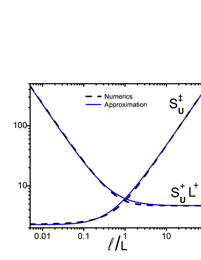
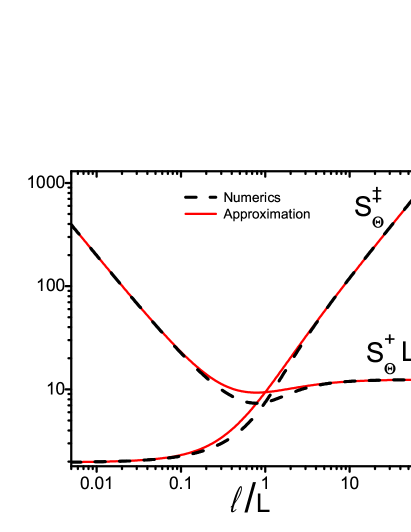
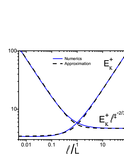
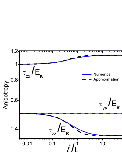
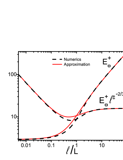
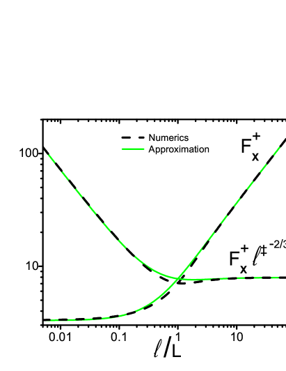
Figure 1: Color online. Log-log plots of the normalized velocity mean shears $S_{\scriptscriptstyle\rm{U}}^{\ddagger}\equiv{\ell^{+}}\,S_{\scriptscriptstyle\rm{U}}^{+}$ and $L^{+}S_{\scriptscriptstyle\rm{U}}^{+}$ (left upper panel), normalized mean-temperature gradients $S_{\scriptscriptstyle\rm{\Theta}}^{\ddagger}\equiv{\ell^{+}}\,S_{\scriptscriptstyle\rm{\Theta}}^{+}$ and $L^{+}S_{\scriptscriptstyle\rm{\Theta}}^{+}$ (right upper panel), the turbulent kinetic energy $E_{\scriptscriptstyle\rm{K}}^{+}$ and $E_{\scriptscriptstyle\rm{K}}^{+}/{\ell^{\ddagger}}^{2/3}$ (left middle panel), partial kinetic energies $\tau_{ii}/E_{\scriptscriptstyle\rm{K}}$ (left middle panel), temperature energy $E_{\theta}^{+}$ and $E_{\theta}^{+}/{\ell^{\ddagger}}^{2/3}$ (left lower panel) and horizontal thermal flux $F_{x}^{+}$ and $F_{x}^{+}/{\ell^{\ddagger}}^{2/3}$ (right lower panel) vs. $\ell^{\ddagger}=\ell/L={\ell^{+}}/L^{+}$. Red and blue solid lines – exact numerical solutions before and after normalization by the large $\ell^{\ddagger}$ asymptotics, black dashed and dot-dashed lines – approximate analytical solutions. The region $\ell\gtrsim L$ may not be realized in the Nature. In this case it has only methodological character.

III.2 Mean velocity and temperature profiles

In principle, integrating the mean shear $S_{\scriptscriptstyle\rm{U}}^{+}$ and the mean temperature gradient $S_{\scriptscriptstyle\rm{\Theta}}^{+}$, one can find the mean velocity and temperature profiles. Unfortunately, to do so we need to know $S_{\scriptscriptstyle\rm{U}}^{+}$ and $S_{\scriptscriptstyle\rm{\Theta}}^{+}$ as functions of the elevation $z$, while in our approach they are found as functions of $\ell/L$. Remember, that the external parameter $\ell$ is the outer scale of turbulence that depends on the elevation $z$: $\ell=\ell(z)$. For $z\ll L$ we can safely take $\ell=z$, however for $z>L$ the function $\ell(z)$ is not found theoretically although it was discussed phenomenologically with support of observational, experimental and numerical data. It is traditionally believed that for $z\gtrsim L$ the scale $\ell$ saturates at some level of the order of $L$ [see, e.g. Eq. (4)].

The resulting plots of $U^{+}$ are shown on Figure 2, upper panel. Even taking $\ell(z)=z$ one gets very similar velocity profile, see Figure 2, lower panel. With $\ell(z)=z$ we find an analytical expression for the mean-velocity profile, using the interpolation Eq. (32b) for $S_{\scriptscriptstyle\rm{U}}^{+}$:

$$U^{+}(z)=\frac{1}{\kappa}\ln\Bigg{[}\frac{z}{z_{u0}\left(1+\sqrt{1+\left(z/L_{2}\right)^{2/3}}\right)^{3}}\Bigg{]}+\frac{z}{L_{1}}\ .$$ (33)

Here $z_{u0}$ is the roughness length. The ratios $L_{j}/L$ are given with our choice of fitting constants.

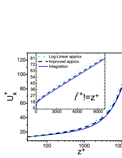
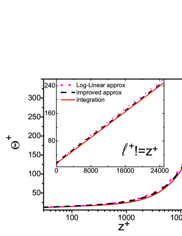
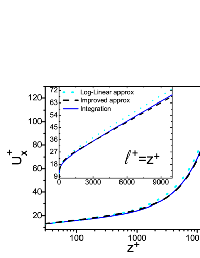
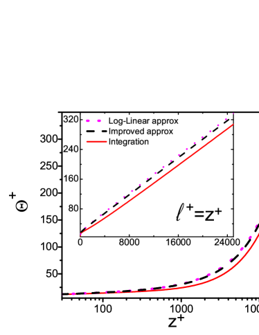
Figure 2: Computed with Eq. (4) (for $d_{1}=d_{2}=1$) plots of $U^{+}$ (blue solid lines on left panels) and $\overline{\Theta}^{\,+}$ (red solid lines on right panels) vs $\ln(z/L)$ and vs. $z/L$ (in inserts) for $L^{+}=1000$. In upper panels $\ell(z)$ is taken from Eq. (4), while in lower panels take $\ell(z)=z$. Log-linear approximation (34a) to all profiles is shown by dotted lines, its improved version (34b) by dashed lines. The region $\ell\gtrsim L$ may not be realized in the Nature. In this case it has only methodological character.

The resulting mean velocity profiles have logarithmic asymptotic for $z<L$ and a linear behavior for $z>L$ in agreement with meteorological observations. Usually the observations are parameterized by a so-called log-linear approximation:

$$U^{+}={\kappa}^{-1}\ln({z}/{z_{u0}})+{z}/{L_{1}}\,,$$ (34a)

which is plotted in Figure 2 by dotted lines. One sees some deviation in the region of intermediate $$z z\gg L L_{2}=L_{1}$$. The reason is that the real profile [see, e.g. Eq. (33)] has a logarithmic term that saturates for , while in the approximation (34a) this term continues to grow. To fix this one can use Eq. (33) (with for simplicity), or even its simplified version

$$U^{+}=\frac{1}{\kappa}\ln\frac{z}{z_{u0}\sqrt{1+(z/L_{1})^{2}}}+\frac{z}{L_{1}}\ .$$ (34b)

This approximation is plotted as a dashed line on Figure 2 for comparison. One sees that our approximation (34b) works much better than the traditional one. Thus we suggest Eq. (34b) for parameterizing meteorological observations.

The temperature profiles in our approach look similar to the velocity ones, see Figure 2, lower panel. They have logarithmic asymptotic for $\ell<L$ and linear behavior for $\ell>L$. Correspondingly, they can be fitted by the log-linear approximation, like (34a), or even better, by improved version of it, like Eq. (34b). Clearly, the values of constant will be different: $\kappa\Rightarrow\kappa_{\scriptscriptstyle\rm{T}}$, $L_{1}\Rightarrow L_{1,\rm T}$, etc.

III.3 Profiles of second-order correlations

The computed profiles of the turbulent kinetic and temperature energies, horizontal thermal flux profile and the anisotropy profiles are shown on Figure 1 in the middle and lower panels. The anisotropy profiles, right middle panel, saturate at $\ell/L\approx 2$, therefore they are not sensitive to the $z$-dependence of $\ell(z)$; even quantitatively one can think of these profiles as if they were plotted as a function of $z/L$.

Another issue is the profiles of $E_{\scriptscriptstyle\rm{K}}^{+}$ (left middle panel) and of $E_{\scriptscriptstyle\rm{\Theta}}$ and $F_{x}^{+}$ (lower panels), that are $\propto(\ell/L)^{2/3}$ for $\ell\gg L$ (if available). With the interpolation formula (4) the profiles of the second order correlations have to saturate at levels corresponding to ${\ell^{\ddagger}}=1$. This sensitivity to the $z$-dependence of $\ell(z)$ makes a comparison of the prediction with available data very desirable.

III.4 Turbulent transport, Richardson and Prandtl numbers

In our notations the turbulent viscosity and thermal conductivity, turbulent Prandtl number, the gradient- and flux-Richardson numbers are

$$\nu_{\scriptscriptstyle\rm{T}} \equiv -\frac{\tau_{xz}}{S_{\scriptscriptstyle\rm{U}}}=\frac{1}{S_{\scriptscriptstyle\rm{U}}^{+}}\equiv C_{\nu}({\ell^{\ddagger}})\frac{\tau_{zz}^{+}}{\gamma_{uu}^{+}}\,,$$ (35a)

$$\chi_{\scriptscriptstyle\rm{T}} \equiv -\frac{F_{z}}{S_{\scriptscriptstyle\rm{\Theta}}}=\frac{1}{S_{\scriptscriptstyle\rm{\Theta}}^{+}}\equiv C_{\chi}({\ell^{\ddagger}})\frac{\tau_{zz}^{+}}{\gamma_{uu}^{+}}\,,$$ (35b)

$$\mbox{Pr}_{\scriptscriptstyle\rm{T}} \equiv \frac{\nu_{\scriptscriptstyle\rm{T}}}{\chi_{\scriptscriptstyle\rm{T}}}=\frac{S_{{}_{\Theta}}^{+}}{S_{{}_{U}}^{+}}=\frac{S_{{}_{\Theta}}^{\ddagger}}{S_{{}_{U}}^{\ddagger}}\,,$$ (35c)

$$\mbox{Ri}_{\rm{grad}} \equiv \frac{\beta S_{{}_{\Theta}}}{S_{{}_{U}}^{2}}=\frac{S_{{}_{\Theta}}^{+}}{L^{+}\,{S_{{}_{U}}^{+}}^{2}}=\frac{{\ell^{\ddagger}}S_{{}_{\Theta}}^{\ddagger}}{{S_{{}_{U}}^{\ddagger}}^{2}}\,,$$ (35d)

$$\mbox{Ri}_{\rm{flux}} \equiv \frac{\beta F_{z}}{\tau_{xy}S_{{}_{U}}}=\frac{1}{L^{+}\,S_{{}_{U}}^{+}}=\frac{{\ell^{\ddagger}}}{S_{{}_{U}}^{\ddagger}}\,,$$ (35e)

$$\mbox{Ri}_{\rm{grad}} = \mbox{Ri}_{\rm{flux}}\,\mbox{Pr}_{\scriptscriptstyle\rm{T}}\ .$$ (35f)

With Eqs. (35a) and (35b) we introduce also two dimensionless functions $C_{\nu}({\ell^{\ddagger}})$ and $C_{\chi}({\ell^{\ddagger}})$ that are taken as ${\ell^{\ddagger}}$-independent constants in the down-gradient transport approximation (3) described in the Introduction. We will show, however, that the functions have a strong dependence on ${\ell^{\ddagger}}$, going to zero in the limit ${\ell^{\ddagger}}\to\infty$ as $1/{\ell^{\ddagger}}^{4/3}$. Therefore this approximation is not valid for large ${\ell^{\ddagger}}$ even qualitatively.

III.4.1 Approximation of down-gradient transport and its violation in stably stratified TBL

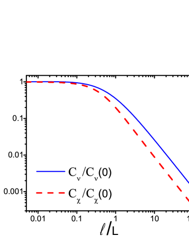
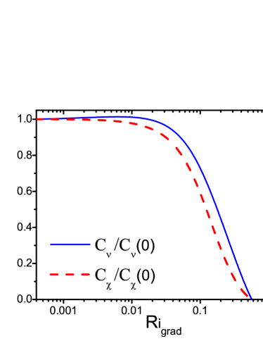
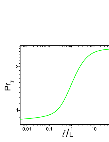
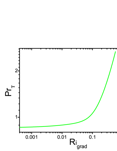
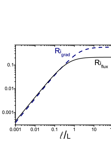
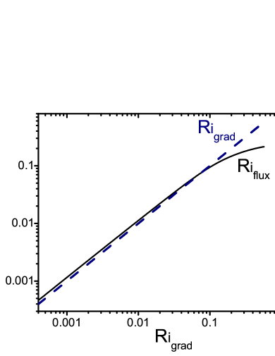
Figure 3: Color online. Log-log plots of “down-gradient coefficient-functions” $C_{\nu}$ (solid blue lines) and $C_{\chi}$ (red dashed lines) – upper panels; turbulent Prandtl number Pr_T (green lines on middle panels) and $\mbox{Ri}_{\rm{flux}}$ (black solid lines), $\mbox{Ri}_{\rm{grad}}$ (black dashed lines) – on lower panels as function of ${\ell^{\ddagger}}=\ell/L$ (left panels) and vs. $\mbox{Ri}_{\rm{grad}}$ (right panels). Notice, that the presented dependencies have qualitative character, and the choice of constants $C_{...}$ depends on the actual functional form $\ell\left(z\right)$. For simplicity, we took $\ell\left(z\right)=z$.The region $\ell\gtrsim L$ may not be realized in the Nature. In this case it has only methodological character.

As we mentioned in the Introduction, the concept of the down-gradient transport assumes that the momentum and thermal fluxes are proportional to the mean velocity and temperature gradients, see Eqs. (3):

$$\tau_{xz}=-\nu_{\scriptscriptstyle\rm{T}}S_{{}_{U}}\,,\quad F_{z}=-\chi_{\scriptscriptstyle\rm{T}}S_{\scriptscriptstyle\rm{\Theta}}\,,$$ (36)

where $\nu_{\scriptscriptstyle\rm{T}}$ and $\chi_{\scriptscriptstyle\rm{T}}$ are effective turbulent viscosity and thermal conductivity, that can be estimated by dimensional reasoning. Equations (3), giving this estimates, include additional physical arguments that vertical transport parameters should be estimated via vertical turbulent velocity, $\sqrt{\tau_{zz}}$, and characteristic vertical scale of turbulence, $\ell_{z}$. The relations between the scales $\ell_{j}$ in different $j$- directions in anisotropic turbulence can be found in the approximation of time-isotropy, according to which

$$\frac{\sqrt{\tau_{xx}}}{\ell_{x}}=\frac{\sqrt{\tau_{yy}}}{\ell_{y}}=\frac{\sqrt{\tau_{zz}}}{\ell_{z}}\equiv\gamma\ \Rightarrow\ \gamma_{uu}\ .$$ (37)

Here $\gamma$ is a characteristic isotropic frequency of turbulence, that for concreteness can be taken as the kinetic energy relaxation frequency $\gamma_{uu}$. The approximation (37) is supported by experimental data, according to which in anisotropic turbulence the ratios $\ell_{i}/\ell_{j}$ ($i\neq j$) are larger then the ratios $\ell_{i}\,\sqrt{\tau_{jj}}\,/\ell_{j}\,\sqrt{\tau_{ii}}$ that are close to unity. With this approximations $\nu_{\scriptscriptstyle\rm{T}}$ and $\chi_{\scriptscriptstyle\rm{T}}$ can be estimated as follows:

$$\nu_{\scriptscriptstyle\rm{T}}=C_{\nu}{\tau_{zz}}/{\gamma_{uu}}\,,\quad\chi_{\scriptscriptstyle\rm{T}}=C_{\chi}{\tau_{zz}}/{\gamma_{uu}}\,,$$ (38)

where, according to the approximation of down-gradient transport, the dimensionless parameters $C_{\nu}$ and $C_{\chi}$ are taken as constants, independent of the level of stratification.

In order to check how the approximation (36), (38) works in the stratified TBL for both fluxes, one can consider Eqs. (36) as the definitions of $\nu_{\scriptscriptstyle\rm{T}}$ and $\chi_{\scriptscriptstyle\rm{T}}$ and Eqs. (38) as the definitions of $C_{\nu}$ and $C_{\nu}$. This gives

$$C_{\nu} \equiv -\frac{\tau_{xz}}{\tau_{zz}}\,\frac{\gamma_{uu}}{S_{{}_{U}}}=\frac{\gamma_{uu}^{+}}{\tau_{zz}^{+}S_{{}_{U}}^{+}}\,,$$ (39a)

$$C_{\chi} \equiv -\frac{F_{x}}{\tau_{zz}}\,\frac{\gamma_{uu}}{S_{\scriptscriptstyle\rm{\Theta}}}=\frac{\gamma_{uu}^{+}}{\tau_{zz}^{+}S_{\scriptscriptstyle\rm{\Theta}}^{+}}\ .$$ (39b)

Recall, that in this paper the down-gradient approximation is not used at all. Instead, we are using exact balance equations for all relevant second order correlation, including $\tau_{xz}$ and $F_{x}$. Substituting our results in the RHS of the definitions (39) we can find, how $C_{\nu}$ and $C_{\chi}$ depend on ${\ell^{\ddagger}}=\ell/L$, that determines the level of stratification in our approach.

The resulting plots of the ratios $C_{\nu}({\ell^{\ddagger}})/C_{\nu}(0)$ and $C_{\chi}({\ell^{\ddagger}})/C_{\chi}(0)$ are shown in the left-upper panel in Figure 3. One sees that the $C_{\nu}({\ell^{\ddagger}})$ and $C_{\chi}({\ell^{\ddagger}})$ can be considered approximately as constants only for $\ell\leq 0.2\,L$. For larger $\ell/L$ both $C_{\nu}({\ell^{\ddagger}})$ and $C_{\chi}({\ell^{\ddagger}})$ rapidly decrease, more or less in the same manner, diminishing by an order of magnitude already for $\ell\approx 2\,L$. For larger $\ell/L$ one can use the asymptotic solution (77), (80) for ${\ell^{\ddagger}}\gg 1$ according to which

$$S_{{}_{U}}^{+}\simeq\frac{1}{L^{+}}\,,\ \gamma_{uu}\simeq\frac{\sqrt{E_{\scriptscriptstyle\rm{K}}^{+}}}{{\ell^{+}}}\simeq\frac{{\ell^{\ddagger}}^{1/3}}{{\ell^{+}}}\,,\ \tau_{zz}\simeq{\ell^{\ddagger}}^{2/3}\ .$$ (40)

This means that both functions vanish as $1/{\ell^{\ddagger}}^{4/3}$:

$$C_{\nu}({\ell^{\ddagger}})\simeq 0.01\left(\frac{L}{\ell}\right)^{4/3}\!\!,\ \ C_{\chi}({\ell^{\ddagger}})\simeq 0.003\left(\frac{L}{\ell}\right)^{4/3}\!\!,$$ (41)

where numerical prefactors account for the accepted values of the dimensionless fit parameters.

The physical reason for the strong dependence of $C_{\nu}$ and $C_{\chi}$ on stratification is as follows: in the RHS of Eq. (24e) for the momentum flux and Eq. (25b) for the vertical heat flux there are two terms. The first ones, proportional to $\tau_{zz}$ and velocity (or temperature) gradients correspond to the approximation (36), giving (in our notations) $C_{\nu}=$const and $C_{\chi}=$const, in agreement with the down-gradient transport concept. However, there are second contributions to the vertical momentum flux $\propto F_{x}$ and to the vertical heat flux, that is proportional to $\beta E_{\theta}$. In our approach both contributions are negative, giving rise the counter-gradient fluxes. What follows from our approach, is that these counter-gradient fluxes cancel (to the leading order) the down-gradient contributions in the limit ${\ell^{\ddagger}}\to\infty$. As a result, in this limit the effective turbulent diffusion and thermal conductivity vanish, making the down-gradient approximation for them (with constant $C_{\nu}$ and $C_{\chi}$) irrelevant even qualitatively for $\ell\gtrsim L$.

In our picture of stable temperature-stratified TBL, the turbulence exists at any elevations, where one can neglect the Coriolis force. Moreover, the turbulent kinetic and temperature energies increase as $(\ell/L)^{2/3}$ for $\ell>L$, see left middle and lower panels in Figure 1. At the same time, the mean velocity and potential temperature change the $(\ell/L)$-dependence from logarithmic lo linear, see Figure 2 and (modified) log-linear interpolation formula (34b). Correspondingly, the shear of the mean velocity and the mean temperature gradient saturate at some elevation (and at some $\ell/L$), and $\mbox{Ri}_{\rm{grad}}$ saturates as well. This predictions agree with large eddy simulation by Zilitinkevich and Esau (2006), see Fig. 5 in ZEKR-paper, where $\mbox{Ri}_{\rm{grad}}$ can be considered as saturating around 0.4 for $z/L\approx 100$.

Nevertheless, our analytical result of saturating $\mbox{Ri}_{\rm{grad}}$ disagree both with the ZEKR model and with various observational, experimental and numerical data, collected in ZEKR-paper, see their Figs. 1, 2, upper panel of Figs. 3 and 4, where various data are plotted as functions of the gradient Richardson number in the interval $(0,100)$. The conditions at which these data were obtained do not correspond to the the situation considered in this paper. Nevertheless, one cannot completely ignore the fact, shown in Fig.1 of ZEKR-paper, that various data concentrate around a linear dependence Pr${}_{\scriptscriptstyle\rm{T}}\sim\mbox{Ri}_{\rm{grad}}$ in the two-decade interval $1<\mbox{Ri}_{\rm{grad}}<100$ (not withstanding the high degree of scatter).

Notice that the turbulent closures of kind used above cannot be applied for strongly stratified flows with $\mbox{Ri}_{\rm{grad}}\gtrsim 1$ (may be even at $\mbox{Ri}_{\rm{grad}}\sim 1$). There are two reasons of that. The first one was mentioned in the Introduction. Namely, for $\mbox{Ri}_{\rm{grad}}\gtrsim 1$ the Brunt-Väisälä frequency $N\equiv\sqrt{\beta S_{\scriptscriptstyle\rm{\Theta}}}$, $N^{+}=\sqrt{\frac{S_{\scriptscriptstyle\rm{\Theta}}^{+}}{L^{+}}}$, is larger then the eddy-turnover frequency and therefore there are weakly decaying Kelvin-Helmholts internal gravity waves which, generally speaking has to be accounted in the momentum and energy balance in TBL.

The second reason, that makes the results very sensitive to the contribution of internal waves follows from the fact that vortical turbulent fluxes vanish (at fixed velocity and temperature gradients). Therefore even relatively small contributions of a different nature to the momentum and thermal fluxes may be important.

The final conclusion is that the TBL modeling at large level of stratification requires accounting for turbulence of the internal waves together with the vortical turbulence, and the analysis of available data calls for serious revision. Definitely, new observations, laboratory and numerical experiments with control of internal wave activity are very likely.

Appendix A Obereck-Boussinesq approximation and conservation laws

A.1 Basic hydrodynamic equations

The system of hydrodynamic equations describing a fluid in which the temperature is not uniform consists of the Navier-Stokes equations for the fluid velocity, $\bm{\mathcal{U}}({\bm{r}},t)$, a continuity equation for the space and time dependent (total) density of the fluid, $\rho({\bm{r}},t)$, and of the heat balance equation for the (total) entropy per unit mass, ${\mathcal{S}}({\bm{r}},t)$, Landau and Lifshitz, 1987 :

$$\rho\frac{{\mathcal{D}}\,\bm{\mathcal{U}}}{{\mathcal{D}}t} = -{\bm{\nabla}}p-{\bm{g}}\,\rho+{\bm{\nabla}}\cdot\mu\,{\bm{\nabla}}\bm{\mathcal{U}}\;,$$ (42a)

$$\frac{\partial{\rho}}{\partial{t}} \!\!+\!\! {\bm{\nabla}}\cdot\left(\rho\,\bm{\mathcal{U}}\right)=0\,,$$ (42b)

$$\rho\frac{{\mathcal{D}}\,{\mathcal{S}}}{{\mathcal{D}}t} = {\bm{\nabla}}\cdot\kappa\,{\bm{\nabla}}{\mathcal{S}}\,,$$ (42c)

$$\frac{{\mathcal{D}}}{{\mathcal{D}}t} \equiv \frac{\partial}{\partial t}+\bm{\mathcal{U}}\cdot{\bm{\nabla}}\ .$$ (42d)

Here ${\mathcal{D}}\,/{\mathcal{D}}t$ is the convective (Lagrangian) derivative, $p$ is the pressure, ${\bm{g}}=-\widehat{\bf{z}}g$ is the vertical acceleration due to gravity, $\mu$ and $\kappa$ are the (molecular) dynamical viscosity and heat conductivity.

These equations are considered with boundary conditions that maintain the solution far from the equilibrium state, where $\bm{\mathcal{U}}={\mathcal{S}}=0$. These boundary conditions are $\bm{\mathcal{U}}=0$ at zero elevation, $\bm{\mathcal{U}}=const$ at a high elevation of a few kilometers. This reflects the existence of a wind at high elevation, but we do not attempt to model the physical origin of this wind in any detail. The only important condition with regards to this wind is that it maintains a momentum flux towards the ground that is prescribed as a function of the elevation. Similarly, we assume that a stable temperature stratification is maintained such that the heat flux towards the ground is prescribed as well. In the entropy balance Eq. (42c) we have already neglected the viscous entropy production term, $\propto\mu{\bm{|}}\nabla\bm{\mathcal{U}}|^{2}$, assuming that the temperature gradients are large enough such that the thermal entropy production term on the RHS of Eq. (42c) dominates. Actually, this assumption is very realistic in our applications. For simplicity of the presentation we restrict ourselves by relatively small elevations and disregard in Eq. (42a) the Coriolis force (for more details, see Wyngaard, 1992).

On the other hand we assume that the temperature and density gradients in the entire turbulent boundary layer are sufficiently small to allow employment of local thermodynamic equilibrium. In other words, we assume the validity of the equation of state, and that the entropy ${\mathcal{S}}$ is a state function of the local values of the density and pressure:

$$\rho=\rho(T,p)\,,\quad{\mathcal{S}}={\mathcal{S}}(\rho,p)\ .$$ (43)

In the same manner we will neglect the temperature dependence of the dissipation parameters $\nu$ and $\kappa$.

Pressure fluctuations caused by turbulent velocity fluctuations ${\bm{u}}$ propagate in a compressible medium with the sound velocity $c_{\rm{s}}$, causing time dependent density fluctuations of the order of $(u/c_{\rm{s}})^{2}\rho_{0}$, where $\rho_{0}$ is the mean density. Assuming that the square of the turbulent Mach number $M_{\scriptscriptstyle\rm{T}}^{2}\equiv(u/c_{\rm{s}})^{2}$ is small compared to unity, we can neglect in Eq. (42b) the partial time derivative: ${\bm{\nabla}}\cdot\left(\rho\,\bm{\mathcal{U}}\right)=0$, see e.g. Landau and Lifshitz, 1987. Even in tropical hurricanes of category five the mean wind velocity $U$ is below 300 Km/h. Usually, the turbulent velocity fluctuations $u$ are less then $U/10$, i.e. even in these extreme conditions $u<30$ Km/h and $M_{\scriptscriptstyle\rm{T}}^{2}<10^{-3}$ (with $c_{\rm{s}}\simeq 1200$ Km/h). Therefore the incompressibility approximation ${\bm{\nabla}}\cdot\left(\rho\,\bm{\mathcal{U}}\right)=0$ is well justified in atmospheric physics. In the ocean where the sound velocity is even larger and water velocities even smaller, this approximation is quite excellent.

A.2 Isentropic basic reference state

In quite air, without turbulence, the pressure and the density depend on the elevation $z$ simply due to gravity. For example, in full thermodynamic equilibrium the temperature is uniform, $z$-independent, and the density decreases exponentially with the elevation. However, this equilibrium model of the atmosphere is not realistic, and cannot be used as a reference state about which the actual dynamics is considered. A much better reference state is a situation in which the entropy is space homogeneous. In this model the thermal conductivity (leading to the temperature homogeneity) is neglected with respect to heat transfer due to the vertical adiabatic mixing of air, leading to a $z$-independent entropy. Following tradition, we refer to the isentropic model as a “basic reference state” and denote this state of the system with a subscript “ _b”:

$${\mathcal{S}}_{\rm{b}}={\mathcal{S}}(\rho_{\rm{\,b}},p_{\rm{\,b}})={\rm const}\,,\quad\rho_{\rm{\,b}}=\rho(T_{\rm{b}},p_{\rm{\,b}})\ .$$ (44)

The first of Eq. (44) relates the gradients of the pressure and density in this state:

$$0={\bm{\nabla}}{\mathcal{S}}_{\rm{b}}=\left(\frac{\partial{\mathcal{S}}_{\rm{b}}}{\partial\rho_{\rm{b}}}\right)_{p}{\bm{\nabla}}\rho_{\rm{b}}+\left(\frac{\partial{\mathcal{S}}_{\rm{b}}}{\partial p_{\rm{b}}}\right)_{\rho}{\bm{\nabla}}p_{\rm{b}}\ .$$ (45a)

Another relation between $$\rho_{\rm{b}} p_{\rm{b}}$$ and follows from the condition of hydrostatic equilibrium:

$${\bm{\nabla}}p_{\rm{b}}={\bm{g}}\rho_{\rm{b}}\ .$$ (45b)

Equations (45) together with the first of Eqs. (44) determine the density, pressure and temperature profiles in the isentropic basic reference state.

A.3 Hydrodynamic equations in generalized Obereck–Boussinesq approximation

A.3.1 Equations of motion

Denote the deviations of the total density, pressure, temperature and entropy from the basic reference state as follows:

$$\hat{\rho}\equiv\rho-\rho_{\rm{\,b}}\,, \hat{p}\equiv p-p_{\rm{\,b}}\,,$$ (46)

$$\hat{T}\equiv T-T_{\rm{\,b}}\,, \hat{{\mathcal{S}}}\equiv{\mathcal{S}}-{\mathcal{S}}_{\rm{\,b}}\,.$$

Following Obereck (1879) and Boussinesq (1903), assume that these deviations are small: $\hat{\rho}\ll\rho_{\rm{\,b}}\,,\quad\hat{p}\ll p_{\rm{\,b}}$. Then one simplifies the full system of hydrodynamic Eqs. (42) and rewrites them in terms of the fluid velocity $\bm{\mathcal{U}}$ and the small deviations $\hat{p}$ and $\hat{{\mathcal{S}}}$ (instead of $\hat{\rho}$). The first step is very simple: because of Eq. (45b)

$${\bm{\nabla}}p-{\bm{g}}\rho={\bm{\nabla}}\hat{p}-{\bm{g}}\,\hat{\rho}\ .$$ (47a)

Next we should relate the deviations $$\hat{p} \hat{\rho} \hat{{\mathcal{S}}}$$, and . In the linear approximation Eq. (43) yields:

$$\hat{{\mathcal{S}}}=\left(\partial{\mathcal{S}}_{\rm{b}}\big{/}\partial p_{\rm{\,b}}\right)_{\rho}\hat{p}+\left(\partial{\mathcal{S}}_{\rm{b}}\big{/}\partial\rho_{\rm{\,b}}\right)_{p}\hat{\rho}\ .$$ (47b)

With the help of Eqs. (45) this gives:

$${\bm{g}}\,\hat{\rho}=\frac{{\bm{\nabla}}\rho_{\rm{b}}}{\rho_{\rm{b}}}\,\hat{p}-{\bm{\beta}}\,\frac{\rho_{\rm{b}}}{c_{\rm{p}}}\,T_{\rm{b}}\,\hat{{\mathcal{S}}}\ .$$ (47c)

Here $${\bm{\beta}}\equiv{\bm{g}}\,\widetilde{\beta} \widetilde{\beta} c_{\rm{p}}$$ is the buoyancy parameter, is the thermal expansion coefficient and is the isobaric specific heat (heat capacity per unit mass at constant pressure) in the basic reference state:

$$\widetilde{\beta}\equiv-\frac{1}{\rho_{\rm{b}}}\left(\frac{\partial\rho_{\rm{b}}}{\partial T_{\rm{b}}}\right)_{p}=-\frac{c_{\rm{p}}}{\rho_{\rm{b}}\,T_{\rm{b}}}\left(\frac{\partial\rho_{\rm{b}}}{\partial{\mathcal{S}}_{\rm{b}}}\right)_{p}\ .$$ (47d)

Now Eq. (47a) in the linear approximation yields:

$${\bm{\nabla}}\hat{p}-{\bm{g}}\rho=\rho_{\rm{b}}\left[{\bm{\nabla}}\left(\frac{p_{\rm{b}}}{\rho_{\rm{b}}}\right)+{\bm{\beta}}\,\frac{T_{\rm{b}}}{c_{p}}\,\hat{{\mathcal{S}}}\right]\ .$$ (47e)

Then Eqs. (42a) can be approximated as:

$$\frac{{\mathcal{D}}\,\bm{\mathcal{U}}}{{\mathcal{D}}t}=-{\bm{\nabla}}\left(\frac{\hat{p}}{\rho_{\rm{b}}}\right)-{\bm{\beta}}\,\frac{T_{\rm{b}}}{c_{p}}\,\hat{{\mathcal{S}}}+\frac{1}{\rho_{b}}{\bm{\nabla}}\cdot\mu\,{\bm{\nabla}}\bm{\mathcal{U}}\ .$$ (48)

A.3.2 Generalized potential temperature

To proceed, we generalize the notion of potential temperature $\Theta$ which is traditionally defined as the temperature that a volume of dry air at a pressure $p(z)$ and temperature $T(z)$ would attain when adiabatically compressed to the pressure $p_{*}$ that exists at zero elevation $z=0$. This potential temperature can be explicitly computed for an ideal gas with the result

$$\Theta(z)\equiv T_{*}\big{(}p_{*}/p(z)\big{)}^{(\gamma-1)/\gamma}\ ,$$ (49)

where $\gamma$ is the ratio of isobaric to isochoric specific heats, $\gamma\equiv c_{\rm{p}}/c_{\rm{v}}$, and $T_{*}$ is the temperature at zero elevation.

We want to generalize the notion of potential temperature for an arbitrary stratified fluid requiring that in the isenotropic basic reference state it would be a constant $\Theta_{*}=T_{*}$. A second requirement is that the definition will agree with Eq. (49) for an ideal gas. Accordingly we define

$$\Theta(z)=T_{*}\exp\left[\left({\mathcal{S}}(z)-{\mathcal{S}}_{\rm b}\right)/c_{\rm{p}}\right]\ .$$ (50)

For more details see also Hauf and Höller (1987). Indeed, if we employ the equation of state and the equation for the entropy of an ideal gas, i.e.

$$p=\rho\,T\,,\quad{\mathcal{S}}=\ln\Bigg{(}\frac{p^{c_{\rm{v}}}}{\rho^{c_{\rm{p}}}}\Bigg{)}+{\rm const}\ ,$$ (51)

one can easily check that Eq. (49) is recaptured.

For small deviations of $\Theta$ from the basic reference state value $T_{*}$, Eq. (50) gives up to linear order:

$$\Theta_{\rm{\,d}}\equiv\Theta-T_{*}=T_{*}\,\hat{{\mathcal{S}}}\big{/}c_{\rm{p}}\ .$$ (52)

Now we can present Eqs. (42a), (42b) (with $\partial\rho_{\rm{\,t}}/\partial t=0$, as explained) and (42c) as follows:

$$\frac{{\mathcal{D}}\,\bm{\mathcal{U}}}{{\mathcal{D}}t} = -{\bm{\nabla}}\left(\frac{p}{\rho_{\rm{b}}}\right)-{\bm{\beta}}\,\Theta_{\rm{\,d}}+\nu\,\Delta\,\bm{\mathcal{U}}\,,$$ (53a)

$$\hskip-28.45274pt{\bm{\nabla}}\cdot\left(\rho_{\rm{b}}\,\bm{\mathcal{U}}\right)=0\,,$$ (53b)

$$\frac{{\mathcal{D}}\,\Theta_{\rm{\,d}}}{{\mathcal{D}}t} = \chi\,\Delta\,\Theta_{\rm{\,d}}\ .$$ (53c)

The dissipative terms are important only in the narrow region of the viscous sublayer, where we can safely neglect the $z$-dependence of $\rho_{\rm{b}}$, $\mu$ and $\kappa$, and consider the dynamical viscosity $\nu=\mu/\rho_{b}$ and dynamical thermal conductivity $\chi=\kappa/\rho_{b}$ as some $z$-independent constants.

Note that for turbulence in liquids (water, etc.) one can simplify these equations further. There one can neglect the effect of adiabatic cooling (together with the compressibility), and simply use another reference state with constant temperature and density:

$$T=T_{*}\,,\quad\rho_{\rm{b}}=\rho_{*}\,,\quad p_{\rm{b}}=p_{*}+g\rho_{*}z\ .$$ (54)

For this reference state standard reasoning (see, e.g. Landau and Lifshitz, 1987) yields the same equations as Eqs. (53) in which again $\widetilde{\beta}$, is given by Eq. (47d) and it is a parameter characterizing a particular fluid. In this case $\rho_{\rm{b}}=\rho_{*}$, independent of $z$, and the potential temperature $\Theta=T$, such that $\Theta_{\rm{\,d}}=T_{\rm{\,d}}$ is a deviation of the total temperature $T$ from its ground (bottom, or whatever) level $T_{*}$.

In our Eq. (53) the situation is more general since we do not assume that reference state has the simple form (54) (with $\rho_{\rm{b}}=\,$const). Importantly, on the RHS of Eq. (53a) the density $\rho_{\rm{b}}(z)$ is operated on by the gradient, and the buoyancy term $-{\bm{\beta}}\Theta_{\rm{\,d}}$ involves $\Theta_{\rm{\,d}}\neq T_{\rm{\,d}}$, the deviation of the potential temperature defined by Eq. (52). This definition for liquids has nothing in common with the standard meteorological definition (49). Notice also that for an ideal gas $\widetilde{\beta}=1/T$, and Eq. (53a) coincide with that suggested in the book Kurbatsky (2000) and used in ZEKR-paper.

It is important to realize that the approximate Eqs. (53) conserve exactly an approximate expression for the total mechanic energy of the system in the dissipation-less limit. Consider the sum of the kinetic, ${\mathcal{E}}_{\scriptscriptstyle\rm{K}}$, and the potential energy ${\mathcal{E}}_{\scriptscriptstyle\rm{P}}$ (calculated in the basic reference state): ${\mathcal{E}}_{\rm{t}}={\mathcal{E}}_{\scriptscriptstyle\rm{K}}+{\mathcal{E}}_{\scriptscriptstyle\rm{P}}$,

$${\mathcal{E}}_{\scriptscriptstyle\rm{K}}\equiv\int d{\bm{r}}\,\rho_{b}\,\frac{|\bm{\mathcal{U}}|^{2}}{2}\,,\quad{\mathcal{E}}_{\scriptscriptstyle\rm{P}}\equiv\int d{\bm{r}}\rho_{b}~{}{\bm{\beta}}\cdot{\bm{r}}~{}\Theta_{d}\ .$$ (55)

One can check by direct substitution that this sum of energies is conserved by of motion Eqs. (53) when $\nu=\chi=0$.

A.4 Potential energy in stratified TBL

In this Appendix we show that the potential energy of a stratified turbulent flow ${\mathcal{E}}_{\scriptscriptstyle\rm{P}}$, Eq. (55), can be presented as the sum of the (time-independent) potential energy of the basic reference state, $\overline{{\mathcal{E}}}_{\scriptscriptstyle\rm{P}}$ and a “turbulent” potential energy, associated with temperature fluctuations, $\widetilde{{\mathcal{E}}}_{\scriptscriptstyle\rm{P}}$ with the density per unit mass $E_{\scriptscriptstyle\rm{P}}={\beta}E_{\theta}/{S_{\Theta}}$:

$$\widetilde{{\mathcal{E}}}_{\scriptscriptstyle\rm{P}}=\int d{\bm{r}}\left(\rho_{\scriptscriptstyle\rm{b}}\beta E_{\theta}/S_{\scriptscriptstyle\rm{\Theta}}\right)\ .$$ (56)

Actually, we want to discuss this issue in a more general case, when the stratification is caused by some “internal” parameter of the fluid, $\xi$, not necessarily the potential temperature. It can be the salinity of water in a sea, the humidity of the air, the concentration of particles co-moving with the fluid as Lagrangian tracers, etc.

In the general case then the equation for the potential energy of a stratified fluid has the form:

$${\mathcal{E}}_{\scriptscriptstyle\rm{P}}=g\int\rho({\bm{r}})z\,dx\,dy\,dz\,,$$ (57a)

In the BRS the potential energy reaches its minimum value referred to as the basic potential energy, $$\overline{{\mathcal{E}}}_{\scriptscriptstyle\rm{P}}$$:

$$\overline{{\mathcal{E}}}_{\scriptscriptstyle\rm{P}}=g\int\rho_{\scriptscriptstyle\rm{b}}(z)z\,dx\,dy\,dz\,,$$ (57b)

where $$\rho_{\scriptscriptstyle\rm{b}}(z) \rho_{\scriptscriptstyle\rm{b}}(z) d\rho_{\scriptscriptstyle\rm{b}}/dz<0$$ is the density profile in BRS. Clearly, in equilibrium the fluid density decreases with the elevation: .

In the turbulent state the density deviates from $\rho_{\scriptscriptstyle\rm{b}}(z)$: $\rho({\bm{r}},t)=\rho_{\scriptscriptstyle\rm{b}}(z)+\widetilde{\rho}({\bm{r}},t)$ and the mean potential energy $\left\langle{\mathcal{E}}_{\scriptscriptstyle\rm{P}}\right\rangle$ exceeds $\overline{{\mathcal{E}}}_{\scriptscriptstyle\rm{P}}$. Now we can write

$$\left\langle{\mathcal{E}}_{\scriptscriptstyle\rm{P}}\right\rangle=\overline{{\mathcal{E}}}_{\scriptscriptstyle\rm{P}}+\widetilde{{\mathcal{E}}}_{\scriptscriptstyle\rm{P}}\ .$$ (57c)

We compute the turbulent potential energy , $\widetilde{{\mathcal{E}}}_{\scriptscriptstyle\rm{P}}$, in the case when the internal parameter $\xi$ (temperature, etc.) is co-moving with the fluid element as a Lagrangian marker. In the Lagrangian approach we can consider $\rho$ as the Lagrangian marker and introduce the variable $z(\rho,t)$, which is understood as an elevation of the fluid element with the density $\rho$. Noticing that $zdz=\frac{1}{2}dz^{2}$, and integrating Eq. (57a) by parts with respect of $z^{2}$, we can present $\left\langle{\mathcal{E}}_{\scriptscriptstyle\rm{P}}\right\rangle$ in the Lagrangian approach as:

$$\left\langle{\mathcal{E}}_{\scriptscriptstyle\rm{P}}\right\rangle=-\frac{g}{2}\int\left\langle[z(\rho,t)]^{2}\right\rangle dx\,dy\,d\rho\ .$$ (58)

As a result of turbulent motion, the elevation $z(\rho,t)$ at given $\rho$ fluctuates and can be decomposed into the mean and fluctuating parts:

$$z(\rho,t)=z_{\scriptscriptstyle\rm{b}}(\rho)+\widetilde{z}(\rho,t)\,,\quad\left\langle\widetilde{z}(\rho,t)\right\rangle=0\ .$$ (59)

Substituting $z^{2}(\rho,t)=z^{2}_{\scriptscriptstyle\rm{b}}+2\,z_{\scriptscriptstyle\rm{b}}\widetilde{z}+\widetilde{z}^{\;2}$ in Eq. (58) we have three contributions to the potential energy. The first one (originating from $z^{2}_{\scriptscriptstyle\rm{b}}$) describes the basic potential energy, Eq. (57b). The second contribution, which is linear in $\widetilde{z}$, disappears because $\left\langle\widetilde{z}\right\rangle=0$. The last one describes the turbulent potential energy:

$$\widetilde{{\mathcal{E}}}_{\scriptscriptstyle\rm{P}}=-\frac{g}{2}\int\left\langle[\widetilde{z}(\rho,t)]^{2}\right\rangle\,dx\,dy\,d\rho\ .$$ (60)

Relating the density fluctuations $\widetilde{\rho}$, around the BRS density profile $\rho_{\scriptscriptstyle\rm{b}}(z)$ (caused by the fluctuations $\widetilde{z}$) with $\widetilde{z}$

$$\delta\rho\equiv\frac{d\rho_{\scriptscriptstyle\rm{b}}(z)}{d\,z}\,\delta z\,,$$ (61)

and returning back to the Eulerian description in Eq. (60) one has:

$$\widetilde{{\mathcal{E}}}_{\scriptscriptstyle\rm{P}}=-\frac{g}{2}\int\left\langle\widetilde{\rho}^{\,2}\right\rangle\Big{[}\frac{d\,\rho_{\scriptscriptstyle\rm{b}}(z)}{dz}\Big{]}^{-1}dx\,dy\,dz\ .$$ (62)

Here we used the transformation formula, similar to Eq. (61): $d\rho=[d\rho_{0}(z)\big{/}d\,z]\,dz$. Equation (62) allows one to introduce a local density of turbulent potential energy per unit mass,

$$E_{\scriptscriptstyle\rm{P}}=-\frac{g}{2}\,\Big{[}\frac{d\,\rho_{\scriptscriptstyle\rm{b}}(z)}{dz}\Big{]}^{-1}\frac{\left\langle{\widetilde{\rho}\,}^{2}\right\rangle}{\rho_{\scriptscriptstyle\rm{b}}}\,,$$ (63a)

such that

$$\widetilde{{\mathcal{E}}}_{\scriptscriptstyle\rm{P}}=\int\rho_{\scriptscriptstyle\rm{b}}E_{\scriptscriptstyle\rm{P}}\,dx\,dy\,dz\ .$$ (63b)

For the particular case of temperature stratification

$$\frac{d\,\rho_{\scriptscriptstyle\rm{b}}(z)}{dz}=\rho_{\scriptscriptstyle\rm{b}}\widetilde{\beta}\,\frac{d\Theta}{dz}\,,\quad\widetilde{\rho}=\rho_{\scriptscriptstyle\rm{b}}\widetilde{\beta}\theta\,,\quad\beta=g\widetilde{\beta}\,,$$ (64)

where $\widetilde{\beta}$ is the thermal expansion coefficient, related, as shown, to the buoyancy parameter $\beta$. With Eqs. (64) and definition of the temperature energy $E_{\theta}=\frac{1}{2}\left\langle\theta^{2}\right\rangle$, Eq. (63a) goes to $E_{\scriptscriptstyle\rm{P}}={\beta}E_{\theta}/{S_{\Theta}}$, as declared.

Appendix B Analysis of the Minimal-Model Balance Equations

B.1 Wall unites and ${\ddagger}$-representation

The Eqs. (27) in the wall units take the form:

$$\tau^{+}_{xx} = E^{+}_{\scriptscriptstyle\rm{K}}-\frac{F^{+}_{z}}{2\,L^{+}\gamma^{+}_{uu}}\,,\quad\tau^{+}_{yy}=\frac{E^{+}_{\scriptscriptstyle\rm{K}}}{2}\,,\quad$$

$$\tau^{+}_{zz} = \frac{E^{+}_{\scriptscriptstyle\rm{K}}}{2}+\frac{F^{+}_{z}}{2\,L^{+}\gamma^{+}_{uu}}\,,$$ (65a)

$$\gamma^{+}_{uu}E^{+}_{\scriptscriptstyle\rm{K}} = \frac{F^{+}_{z}}{L^{+}}-\tau^{+}_{xz}S^{+}_{{}_{U}}\,,$$ (65b)

$$4\,\widetilde{C}_{\scriptscriptstyle\rm{RI}}\,\gamma^{+}_{uu}\tau^{+}_{xz} = \frac{F^{+}_{x}}{L^{+}}-\tau^{+}_{zz}\,S^{+}_{{}_{U}}\,,$$ (65c)

$$C_{\theta\theta}\,\gamma^{+}_{uu}E^{+}_{\theta} = -F^{+}_{z}\,S^{+}_{{}_{\Theta}}\,,$$ (65d)

$$C_{u\theta}\,\gamma^{+}_{uu}F^{+}_{x} = -\tau^{+}_{xz}S^{+}_{{}_{\Theta}}-C_{\scriptscriptstyle\rm{SU}}F^{+}_{z}\,S^{+}_{{}_{U}}\,,$$ (65e)

$$C_{u\theta}\,\gamma^{+}_{uu}F^{+}_{z} = -\tau^{+}_{zz}S^{+}_{{}_{\Theta}}-2\,\frac{C_{\scriptscriptstyle\rm{E\Theta\,}}E^{+}_{\theta}}{L^{+}}\,,$$ (65f)

with

$$\gamma^{+}_{uu}=c_{uu}{\sqrt{E^{+}_{\scriptscriptstyle\rm{K}}}\over\ell^{+}}\,,\quad\tau^{+}_{xz}=F^{+}_{z}=-1\ .$$ (65g)

Outside of the viscous region, the problem has only one characteristic length, the Monin-Obukhov scale $L$. Correspondingly, one expects that the only dimensionless parameter that governs the turbulent statistics in this region should be the ratio of the outer scale of turbulence, $\ell$, to the Monin-Obukhov length-scale $L$, which we denote as $\ell^{\ddagger}\equiv{\ell}/{L}=\ell^{+}/L^{+}$. Indeed, introducing “${\ddagger}$-objects”:

$$\ell^{\ddagger}\equiv{\ell}/{L}\,,\quad S_{{}_{U}}^{\ddagger}\equiv S_{{}_{U}}^{+}\ell^{+}\,,\ S_{{}_{\Theta}}^{\ddagger}\equiv S_{{}_{\Theta}}^{+}\ell^{+}\,,$$ (66)

one rewrites the balance Eqs. (65) as follows:

$$\hskip-36.98866pt\tau^{+}_{xx}=E^{+}_{\scriptscriptstyle\rm{K}}+{\ell^{\ddagger}}/2c_{uu}\sqrt{E^{+}_{\scriptscriptstyle\rm{K}}}\,,\quad\tau^{+}_{yy}={E^{+}_{\scriptscriptstyle\rm{K}}}/2\,,$$ (67a)

$$\hskip-36.98866pt2\,\tau^{+}_{zz}={E^{+}_{\scriptscriptstyle\rm{K}}}-{\ell^{\ddagger}}/c_{uu}\sqrt{E^{+}_{\scriptscriptstyle\rm{K}}}\,,~{}~{}~{}~{}$$ (67c)

$$\hskip-36.98866ptc_{uu}{E^{+}_{\scriptscriptstyle\rm{K}}}^{3/2}=\ell^{\ddagger}F^{+}_{z}-\tau^{+}_{xz}S^{\ddagger}_{{}_{U}}\,,$$

$$\hskip-36.98866pt4\,\widetilde{C}_{\scriptscriptstyle\rm{RI}}\,c_{uu}\sqrt{E^{+}_{\scriptscriptstyle\rm{K}}}\tau^{+}_{xz}=\ell^{\ddagger}F^{+}_{x}-\tau^{+}_{zz}\,S^{\ddagger}_{{}_{U}}\,,$$ (67d)

$$\hskip-36.98866ptC_{\theta\theta}\,c_{uu}\sqrt{E^{+}_{\scriptscriptstyle\rm{K}}}E^{+}_{\theta}=-F^{+}_{z}\,S^{\ddagger}_{{}_{\Theta}}\,,$$ (67e)

$$\hskip-36.98866ptC_{u\theta}\,c_{uu}\sqrt{E^{+}_{\scriptscriptstyle\rm{K}}}F^{+}_{x}=-\tau^{+}_{xz}S^{\ddagger}_{{}_{\Theta}}-C_{\scriptscriptstyle\rm{SU}}F^{+}_{z}\,S^{\ddagger}_{{}_{U}}\,,$$ (67f)

$$\hskip-36.98866ptC_{u\theta}\,c_{uu}\sqrt{E^{+}_{\scriptscriptstyle\rm{K}}}F^{+}_{z}=-\tau^{+}_{zz}S^{\ddagger}_{{}_{\Theta}}-2\,C_{\scriptscriptstyle\rm{E\Theta}}\,\ell^{\ddagger}E^{+}_{\theta}\,,$$ (67g)

B.2 Polynomial formulation of balance Eqs. (67)

In Sect. B.4.2 we justify the simple choice

$$C_{\scriptscriptstyle\rm{E\Theta}}\approx-2\,C_{\theta\theta}\big{/}3\,,$$ (68)

which is used presently. With it the equations  (31) [except of (31d)] yield expressions for $S_{{}_{U}}^{\ddagger}$, $S_{\scriptscriptstyle\rm{\Theta}}^{\ddagger}$, $E_{\theta}^{+}$ and $F_{x}^{+}$ as functions of $\ell^{\ddagger}$ and $X$:

$$X \equiv \sqrt{E_{\scriptscriptstyle\rm{K}}^{+}(\ell^{\ddagger})}\,,$$ (69a)

$$S^{\ddagger}_{{}_{U}}(\ell^{\ddagger}) = {\ell^{\ddagger}F^{+}_{z}-c_{uu}X^{3}}\over{\tau^{+}_{xz}}\,,$$ (69b)

$$S^{\ddagger}_{\scriptscriptstyle\rm{\Theta}}(\ell^{\ddagger}) = -\frac{6\,c_{uu}^{2}C_{u\theta}\,X^{2}F^{+}_{z}}{3\,c_{uu}X^{3}+11\,\ell^{\ddagger}F^{+}_{z}}\,,$$ (69c)

$$E^{+}_{\theta}(\ell^{\ddagger}) = -\frac{S^{\ddagger}_{\scriptscriptstyle\rm{\Theta}}}{c_{uu}C_{\theta\theta}X}F^{+}_{z},$$ (69d)

$$F^{+}_{x}(\ell^{\ddagger}) = -\frac{\tau^{+}_{xz}S^{\ddagger}_{\scriptscriptstyle\rm{\Theta}}+C_{\scriptscriptstyle\rm{SU}}S^{\ddagger}_{{}_{U}}F^{+}_{z}}{c_{uu}\,C_{u\theta}X}\ .$$ (69e)

Substituting Eqs. (69) into the remaining Eq. (31d) one gets an equation for $E_{\scriptscriptstyle\rm{K}}$ which can be represented as the $9^{\textrm{th}}$ order polynomial for $X\equiv\sqrt{E_{\scriptscriptstyle\rm{K}}^{+}(\ell^{\ddagger})}$:

$$-12\,c_{uu}^{2}C_{u\theta}\,{\tau^{+}_{xz}}^{2}\ell^{\ddagger}F^{+}_{z}X^{2}+\left(3\,c_{uu}X^{3}+11\,{\ell^{\ddagger}}F^{+}_{z}\right)~{}~{}~{}~{}~{}~{}~{}$$

$$\times\Big{\{}8\,c_{uu}^{2}\widetilde{C}_{\scriptscriptstyle\rm{RI}}C_{u\theta}\,{\tau^{+}_{xz}}^{2}X^{2}-\left(c_{uu}X^{3}-{\ell^{\ddagger}}F^{+}_{z}\right)$$ (70)

$$\times\big{[}\left(2\,C_{\scriptscriptstyle\rm{SU}}+C_{u\theta}\right)\ell^{\ddagger}F^{+}_{z}+c_{uu}C_{u\theta}X^{3}\big{]}\Big{\}}=0\ .$$

This equation can be solved numerically to find the function $X(\ell^{\ddagger})$. After that Eqs. (69) allow to find all the required correlations as functions of $\ell^{\ddagger}$, see red solid lines in Figure 1.

The following subsections are dedicated to finding of an approximate analytical solutions for all correlations that will describe their $\ell^{\ddagger}$-dependence with reasonable accuracy. First we will find in the next Sec. B.3 the solution of Eqs. (69) and (70) for $\ell^{\ddagger}=0$ , corrected up to linear order in $\ell^{\ddagger}$. Then, in Sec. B.4.2 we will find the asymptotic solution for $\ell^{\ddagger}\to\infty$ with corrections, linear in the small parameter $\delta=2(c_{uu}/\ell^{\ddagger})^{4/3}$.

B.3 Solution for neutral and weak stratification

For neutral stratification, when $\ell^{\ddagger}=0$, Eq. (70) trivially yields:

$$X=X_{0}=(8\,\widetilde{C}_{\scriptscriptstyle\rm{RI}})^{1/4}\,,\quad E_{\scriptscriptstyle\rm{K}}^{+}={E_{\scriptscriptstyle\rm{K,\scriptstyle{0}}}^{+}}\equiv 2\sqrt{2\,\widetilde{C}_{\scriptscriptstyle\rm{RI}}}\ .$$ (71a)

With Eqs. (69) this gives:

$$S^{\ddagger}_{\scriptscriptstyle\rm{U,{\scriptstyle{0}}}} = -{{c_{uu}X^{3}_{0}}\over{\tau^{+}_{xz}}}\,,$$ (71b)

$$S^{\ddagger}_{\scriptscriptstyle\rm{\Theta,{\scriptstyle{0}}}} = -\frac{2\,c_{uu}C_{u\theta}\,F^{+}_{z}}{X_{0}}\,,$$ (71c)

$$E^{+}_{\theta,{\scriptstyle{0}}} = -\frac{S^{\ddagger}_{\scriptscriptstyle\rm{\Theta,{\scriptstyle{0}}}}F^{+}_{z}}{c_{uu}C_{\theta\theta}X_{0}}\,,$$ (71d)

$$F^{+}_{x,0} = -\frac{\tau^{+}_{xz}S^{\ddagger}_{\scriptscriptstyle\rm{\Theta,{\scriptstyle{0}}}}+C_{\scriptscriptstyle\rm{SU}}S^{\ddagger}_{\scriptscriptstyle\rm{U,{\scriptstyle{0}}}}F^{+}_{z}}{c_{uu}\,C_{u\theta}X_{0}}\ .$$ (71e)

Remembering that $S_{\scriptscriptstyle\rm{U,\scriptstyle{0}}}^{\ddagger}=1/\kappa$ and using experimental values in the lag-law region $E^{+}_{\scriptscriptstyle\rm{K,{\scriptstyle{0}}}}\approx 3.42$ and $\kappa\approx 0.436$ one finds:

$$\widetilde{C}_{\scriptscriptstyle\rm{RI}}\approx 1.46\,,\quad c_{uu}\approx 0.36\ .$$ (72)

Using the relationship between $E_{\scriptscriptstyle\rm{K,{\scriptstyle{0}}}}^{+}$ and $\kappa$ as suggested in L’vov et al. (2006), $E_{\scriptscriptstyle\rm{K,{\scriptstyle{0}}}}^{+}=18\kappa^{2}$, one finds a relationship between these two constants,

$$4\sqrt{2}\,c_{uu}\widetilde{C}_{\scriptscriptstyle\rm{RI}}=3\,,$$ (73)

which agrees with the known values (72) with an accuracy that is better then 1%.

In the case of weak stratification one can develop a perturbative approach to Eq. (70), using $\ell^{\ddagger}\ll 1$ as a small parameter, to develop a solution in the form of a Taylor series in powers of $\ell^{\ddagger}$:

$$X=X_{0}+X_{1}{\ell^{\ddagger}}+X_{2}{\ell^{\ddagger}}^{2}+\dots$$ (74a)

For our purpose only the linear term in $$\ell^{\ddagger}$$ is required:

$$X_{1}=-F_{z}^{+}\frac{2\,{\tau^{+}_{xz}}^{2}C_{u\theta}+C_{\scriptscriptstyle\rm{SU}}X^{4}_{0}}{2\,c_{uu}C_{u\theta}X^{6}_{0}}\,,$$ (74b)

where $X_{0}$ is given by Eq. (71a). Using now the exact relations (69) with $E_{\scriptscriptstyle\rm{K}}^{+}=X^{2}$ one can immediately find the linear terms in $\ell^{\ddagger}$ in the expansions for $E_{\scriptscriptstyle\rm{K}}^{+}(\ell^{\ddagger})$, $S_{{}_{U}}^{\ddagger}$, $S_{\scriptscriptstyle\rm{\Theta}}^{\ddagger}$, $E_{\theta}^{+}$ and $F_{x}^{+}$:

$$E_{\scriptscriptstyle\rm{K}}^{+} = E^{+}_{\scriptscriptstyle\rm{K,{\scriptstyle{0}}}}+E^{+}_{\scriptscriptstyle\rm{K,{\scriptstyle{1}}}}\ell^{\ddagger}+\dots\ ,$$ (75a)

$$S_{{}_{\Theta}}^{\ddagger} = S^{\ddagger}_{{}_{\Theta,{\scriptstyle{0}}}}+S^{\ddagger}_{{}_{\Theta,{\scriptstyle{1}}}}\ell^{\ddagger}+\dots\ ,\quad\mbox{etc.}$$ (75b)

where

$$E_{\scriptscriptstyle\rm{K,{\scriptstyle{1}}}}^{+} = -\frac{F^{+}_{z}}{c_{uu}E^{+\,1/2}_{\scriptscriptstyle\rm{K,{\scriptstyle{0}}}}}\left(2\frac{{\tau^{+}_{xz}}^{2}}{E^{+\,2}_{\scriptscriptstyle\rm{K,{\scriptstyle{0}}}}}+\frac{C_{\scriptscriptstyle\rm{SU}}}{C_{u\theta}}\right),$$ (76a)

$$E_{\theta,{\scriptstyle{1}}}^{+} = \frac{2\,{F^{+}_{z}}^{2}}{3\,c_{uu}E^{+\,5/2}_{\scriptscriptstyle\rm{K,{\scriptstyle{0}}}}}\left(6\frac{{\tau^{+}_{xz}}^{2}}{E^{+\,2}_{\scriptscriptstyle\rm{K,{\scriptstyle{0}}}}}-11+3\frac{C_{\scriptscriptstyle\rm{SU}}}{C_{u\theta}}\right),$$ (76b)

$$S^{+}_{\scriptscriptstyle\rm{U,{\scriptstyle{1}}}} = \frac{F^{+}_{z}}{\tau^{+}_{xz}}\left(1+3\frac{{\tau^{+}_{xz}}^{2}}{E^{+\,2}_{\scriptscriptstyle\rm{K,{\scriptstyle{0}}}}}+\frac{3}{2}\frac{C_{\scriptscriptstyle\rm{SU}}}{C_{u\theta}}\right)\,,$$ (76c)

$$S^{\ddagger}_{\scriptscriptstyle\rm{\Theta,{\scriptstyle{1}}}} = -\frac{{2\,C_{u\theta}F^{+}_{z}}^{2}}{3\,E^{+\,2}_{\scriptscriptstyle\rm{K,{\scriptstyle{0}}}}}\left(3\,\frac{{\tau^{+}_{xz}}^{2}}{E^{+\,2}_{\scriptscriptstyle\rm{K,{\scriptstyle{0}}}}}-11+\frac{3}{2}\frac{C_{\scriptscriptstyle\rm{SU}}}{C_{u\theta}}\right),~{}~{}~{}~{}~{}~{}~{}$$ (76d)

$$F_{x,{\scriptstyle{1}}}^{+} = -\frac{\tau^{+}_{xz}S^{\ddagger}_{\scriptscriptstyle\rm{\Theta,{\scriptstyle{1}}}}+C_{\scriptscriptstyle\rm{SU}}F^{+}_{z}S^{\ddagger}_{\scriptscriptstyle\rm{U,{\scriptstyle{1}}}}}{c_{uu}C_{u\theta}\sqrt{E^{+}_{\scriptscriptstyle\rm{K,{\scriptstyle{0}}}}}}$$

$$+\frac{\tau^{+}_{xz}S^{\ddagger}_{\scriptscriptstyle\rm{\Theta,{\scriptstyle{0}}}}+C_{\scriptscriptstyle\rm{SU}}F^{+}_{z}S^{\ddagger}_{\scriptscriptstyle\rm{U,{\scriptstyle{0}}}}}{2\,c_{uu}C_{u\theta}\sqrt{E^{+}_{\scriptscriptstyle\rm{K,{\scriptstyle{0}}}}}}\frac{E^{+}_{\scriptscriptstyle\rm{K,{\scriptstyle{1}}}}}{E^{+}_{\scriptscriptstyle\rm{K,{\scriptstyle{0}}}}}\ .$$

B.4 Solution for strong sratification

To analyze Eqs. (65) for large $\ell^{\ddagger}$, introduce new variables for the second order correlations $e_{\scriptscriptstyle\rm{K}}$, $e_{\theta}$, and $f_{x}$, according to

$$E^{+}_{\scriptscriptstyle\rm{K}} = {\left(e_{\scriptscriptstyle\rm{K}}{\ell}^{\ddagger}\right)}^{2/3},\quad E^{+}_{\theta}=\frac{e_{\theta}}{\sqrt[3]{e}_{\scriptscriptstyle\rm{K}}}\,{{\ell}^{\ddagger}}^{2/3}=\frac{e_{\theta}\ell^{\ddagger}}{\sqrt{E_{\scriptscriptstyle\rm{K}}^{+}}}\,,$$

$$F^{+}_{x} = \frac{f_{x}}{\sqrt[3]{e}_{\scriptscriptstyle\rm{K}}}\,{{\ell}^{\ddagger}}^{2/3}=\frac{f_{x}\ell^{\ddagger}}{\sqrt{E_{\scriptscriptstyle\rm{K}}^{+}}}\ .$$ (77)

In these variables Eqs. (65) take the form:

$$c_{uu}e_{\scriptscriptstyle\rm{K}} = {L^{+}S_{\scriptscriptstyle\rm{U}}^{+}}-1\,,$$ (78a)

$$4\,\delta\,\widetilde{C}_{\scriptscriptstyle\rm{RI}}\,(c_{uu}\,e_{\scriptscriptstyle\rm{K}})^{2/3} = \left(c_{uu}e_{\scriptscriptstyle\rm{K}}-1\right){L^{+}S_{\scriptscriptstyle\rm{U}}^{+}}-2\,c_{uu}\,f_{x},~{}~{}~{}~{}~{}~{}~{}~{}~{}~{}$$ (78b)

$$C_{\theta\theta}\,c_{uu}e_{\theta} = {L^{+}S_{\scriptscriptstyle\rm{\Theta}}^{+}}\,,$$ (78c)

$$C_{u\theta}\,c_{uu}f_{x} = L^{+}(S_{\scriptscriptstyle\rm{\Theta}}^{+}+C_{\scriptscriptstyle\rm{SU}}\,S_{\scriptscriptstyle\rm{U}}^{+})\,,$$ (78d)

$$\delta\,C_{u\theta}\,(c_{uu}\,e_{\scriptscriptstyle\rm{K}})^{2/3} = L^{+}S_{\scriptscriptstyle\rm{\Theta}}^{+}\left(c_{uu}e_{\scriptscriptstyle\rm{K}}-1\right)$$ (78e)

$$+4\,C_{\scriptscriptstyle\rm{E\Theta}}\,c_{uu}e_{\theta}\,,$$

with a small parameter $\delta$

$$\delta\equiv 2\,\Big{(}\frac{c_{uu}}{\ell^{\ddagger}}\Big{)}^{4/3}\ ,$$ (79)

appearing in the LHS of the equations for the vertical momentum and thermal fluxes.

B.4.1 Asymptotic solution for $\ell^{\ddagger}\to\infty$

In the limit $\ell^{\ddagger}\to\infty$, one takes $\delta=0$ in Eqs. (78) and gets an asymptotic solution (denoted by “^∞”)

$$e^{\infty}_{\scriptscriptstyle\rm{K}} = \frac{1}{c_{uu}}\!\left(1-4\frac{C_{\scriptscriptstyle\rm{E\Theta}}}{C_{\theta\theta}}\right),$$ (80a)

$$S_{\scriptscriptstyle\rm{U}}^{+\infty} = \frac{2}{L^{+}}\left(1-2\frac{C_{\scriptscriptstyle\rm{E\Theta}}}{C_{\theta\theta}}\right),$$ (80b)

$$S_{\scriptscriptstyle\rm{\Theta}}^{+\infty} = -S_{\scriptscriptstyle\rm{U}}^{+\infty}\Big{(}C_{\scriptscriptstyle\rm{SU}}+2C_{u\theta}\frac{C_{\scriptscriptstyle\rm{E\Theta}}}{C_{\theta\theta}}\Big{)},$$ (80c)

$$e_{\theta}^{\infty} = \frac{L^{+}S_{\scriptscriptstyle\rm{\Theta}}^{+\infty}}{c_{uu}C_{\theta\theta}}\,,$$ (80d)

$$f_{x}^{\infty} = -2\frac{C_{\scriptscriptstyle\rm{E\Theta}}}{C_{\theta\theta}}\frac{L^{+}S_{\scriptscriptstyle\rm{U}}^{+\infty}}{c_{uu}}\ .$$ (80e)

The physics of the problem requires that ${S_{\scriptscriptstyle\rm{U}}^{+}}$ $S_{{}_{\Theta}}^{+}$, $e_{\scriptscriptstyle\rm{K}}$ and $e_{\theta}$ be positively definite. This constraints the possible values of the fitting constants. With $C_{\scriptscriptstyle\rm{E\Theta}}<0$, Eq. (68), we have:

$$c_{uu}>0\,,\quad C_{\theta\theta}>0\,,\quad C_{u\theta}>C_{\scriptscriptstyle\rm{SU}}\,C_{\theta\theta}/2|C_{{}_{E\theta}}|\ .$$ (81)

Notice, that the maximal value of Ri_flux, [defined in Eq. (35e)], which we denote as Ri${}_{\rm{f,\,max}}$, corresponds to $\ell^{\ddagger}\to\infty$ and equals to $1/L^{+}S_{\scriptscriptstyle\rm{U}}^{+\infty}$. Taking for $C_{E\theta}=-2/3$ according to the estimate $C_{{}_{E\theta}}\approx-2/3$, and, following ZEKR-paper, accept $C_{\theta\theta}=1$, one gets Ri${}_{\rm{f,\,max}}=3/14\approx 0.21$ in agreement with the experimental value (which is between 0.20 and 0.25). With the choice

$$C_{E\theta}=-2/3\,,\quad C_{\theta\theta}=1\ .$$ (82)

Equations (80b) give the following predictions:

$$e_{\scriptscriptstyle\rm{K}}^{\infty}\!\! = \!\!\frac{11}{3\,c_{uu}}\approx 10.1\,,\ \Rightarrow\ E_{\scriptscriptstyle\rm{K}}^{+}\approx 4.7\,{{\ell^{\ddagger}}}^{2/3}\,,$$ (83a)

$$S_{\scriptscriptstyle\rm{U}}^{+\infty}\!\! = \!\!\frac{14}{3\,L^{+}}\,,\ \ \Rightarrow\ \ \max\mbox{Ri}_{\rm{flux}}=\frac{3}{14}\approx 0.21\,,~{}~{}~{}~{}~{}~{}~{}$$ (83b)

$$S_{\scriptscriptstyle\rm{\Theta}}^{+\infty}\!\! = \!\!-S_{\scriptscriptstyle\rm{U}}^{+\infty}\left(C_{\scriptscriptstyle\rm{SU}}-\frac{4}{3}C_{u\theta}\right),$$ (83c)

$$e_{\theta}^{\infty}\!\! = \!\!L^{+}\!S_{\scriptscriptstyle\rm{\Theta}}^{+\infty}/{c_{uu}}\,,$$ (83d)

$$f_{x}^{\infty}\!\! = \!\!\frac{4}{3}\frac{L^{+}S_{\scriptscriptstyle\rm{U}}^{+\infty}}{c_{uu}}\approx 17.2\,,\ \Rightarrow\ F_{x}^{+}\approx 6.7\,{\ell^{\ddagger}}^{2/3}.~{}~{}~{}~{}$$ (83e)

B.4.2 Expansion around $\ell^{\ddagger}\to\infty$

The small parameter in Eqs. (78) allows one to find the solution as Taylor series in $\delta\ll 1$:

$${S_{\scriptscriptstyle\rm{\Theta}}^{+}}={S_{\scriptscriptstyle\rm{\Theta}}^{+}}^{\infty}+S_{\scriptscriptstyle\rm{\Theta,1}}^{+\infty}\delta+S_{\scriptscriptstyle\rm{\Theta,2}}^{+\infty}\delta^{2}+\dots\,,\ \mbox{etc.}$$ (84a)

For our purposes we need to know only the linear terms in $$\delta$$:

$$e_{\scriptscriptstyle\rm{K,1}}^{\infty} = \frac{3}{11}C_{u\theta}\frac{e_{\scriptscriptstyle\rm{K}}^{\infty}}{S^{+\infty}_{\scriptscriptstyle\rm{\Theta}}L^{+}}\,,$$ (84b)

$$S^{+\infty}_{{}_{U},_{1}} = \frac{C_{u\theta}}{S^{+\infty}_{\scriptscriptstyle\rm{\Theta}}{L^{+}}^{2}}\,,$$ (84c)

$$S^{+\infty}_{\scriptscriptstyle\rm{\Theta,1}} = \frac{C_{u\theta}}{L^{+}}\left(\frac{11\,C_{u\theta}-3\,C_{\scriptscriptstyle\rm{SU}}}{{3\,S_{\scriptscriptstyle\rm{\Theta}}^{+\infty}}L^{+}}-2\widetilde{C}_{\scriptscriptstyle\rm{RI}}\right),$$ (84d)

$$e_{\theta,_{1}}^{\infty} = \frac{S^{+\infty}_{\scriptscriptstyle\rm{\Theta,1}}L^{+}}{c_{uu}}\,,$$ (84e)

$$f_{x,_{1}}^{\infty} = C_{u\theta}\frac{e_{\scriptscriptstyle\rm{K}}^{\infty}}{S_{\scriptscriptstyle\rm{\Theta}}^{+\infty}L^{+}}-2\frac{\widetilde{C}_{\scriptscriptstyle\rm{RI}}}{c_{uu}}.$$ (84f)

Appendix C On the closure problem of triple correlations via second order correlations

Let us look more carefully at the approximation (26), which is

$$\gamma_{uu} = c_{uu}\sqrt{E_{\scriptscriptstyle\rm{K}}}\big{/}\ell\,,\quad\gamma_{\scriptscriptstyle\rm{RI}}=C_{\scriptscriptstyle\rm{RI}}\gamma_{uu}\,,$$ (85)

$$\widetilde{\gamma}_{\scriptscriptstyle\rm{RI}} = \widetilde{C}_{\scriptscriptstyle\rm{RI}}\gamma_{\scriptscriptstyle\rm{RI}}\,,\gamma_{\theta\theta}=C_{\theta\theta}\gamma_{uu}\,,\quad\gamma_{\scriptscriptstyle\rm{RD}}=C_{u\theta}\gamma_{uu}\ .$$

The dimensional reasoning that leads to this approximation is questionable for problems having a dimensionless parameter ${\ell^{\ddagger}}$. Generally speaking, all “constants” $c_{...}$ and $C_{...}$ in Eq. (85) can be any functions of ${\ell^{\ddagger}}$. Presently we just hope that a possible ${\ell^{\ddagger}}$ dependence of these functions is relatively weak and does not affect the qualitative picture of the phenomenon.

Moreover, even the assumption (19a) that the dissipation of the thermal flux $\epsilon_{i}$ is proportional to the thermal flux and the assumption (19b) that the dissipation of $E_{\theta}$, $\varepsilon\propto E_{\theta}$ are also questionable. Formally speaking, one cannot guarantee that the tripple cross-correlator $\left\langle\theta uu\right\rangle^{+}$ that estimates $\epsilon^{+}$, can be (roughly speaking) decomposed like $\left\langle u\theta\right\rangle\sqrt{\left\langle uu\right\rangle}$, i.e really proportional to $F=\left\langle u\theta\right\rangle$ as it stated in Eq. (19a). Theoretically, one cannot exclude the decomposition $\left\langle\theta uu\right\rangle\sim\left\langle uu\right\rangle\sqrt{\left\langle\theta\theta\right\rangle}$, i.e. a contribution to $\epsilon\propto E_{\scriptscriptstyle\rm{K}}$. Similarly, the dissipation $\varepsilon$ in the balance (10c) of $E_{\theta}$, that is determined by the correlator (19b), is $\propto\left\langle\theta\theta u\right\rangle$, as it follows from the decomposition $\left\langle\theta\theta u\right\rangle\sim\left\langle\theta\theta\right\rangle\sqrt{\left\langle uu\right\rangle}$ and is stated in Eq. (19b). This correlator allows, for example, the decomposition $\left\langle\theta\theta u\right\rangle\sim\left\langle\theta u\right\rangle\sqrt{\left\langle\theta\theta\right\rangle}$, i.e. contribution to $\varepsilon\propto F$. This discussion demonstrates, that the situation with the dissipation rates is not so simple, as one may think and thus requires careful theoretical analysis that is in our agenda for future work. Our preliminary analysis of this problem shows that all fitting constants are indeed functions of ${\ell^{\ddagger}}$. Fortunately, they vary within finite limits in the entire interval $0\leq{\ell^{\ddagger}}<\infty$. Therefore we propose that the approximations used in this paper preserve the qualitative picture of the phenomenon. Once again, the traditional down-gradient approximation does not work even qualitatively because corresponding “constants” $C_{\nu}$ and $C_{\chi}$ vanish in the limit ${\ell^{\ddagger}}\to\infty$.

References

• (1) Boussinesq, J.: 1903, The’orique Analytique de la Chaleur, Vol. 2. Gauthier-Villars, Paris.
• (2) Cheng, Y., Canuto, V. M., and Howard, A. M., 2002: An improved model for the turbulent PBL, J. Atm. Sci., 59, 1550-1565.
• (3) Canuto, V. M., 2002: Critical Richardson numbers and gravity waves, Astronomy & Astrophysics, 384, 1119-1123.
• (4) Elperin, T., Kleeorin, N., Rogachevskii, I., and Zilitinkevich, S., 2002: Formation of large-scale semi-organized structures in turbulent convection. Phys. Rev. E, 66, 066305.
• (5) Hanazaki, H., and Hunt, J. C. R., 2004: Structure of unsteady stably stratified turbulence with mean shear. J. Fluid Mech., 507, 1-42.
• (6) Hauf, T., and Höller, H.: 1987, Entropy and Potential Temperature, J. of Atm. Sci., 44, 2887-2901.
• (7) Hunt, J. C. R., Stretch, D. D., and Britter, R. E., 1988: Length scales in stably stratified turbulent flows and their use in turbulence models. In: Proc. I.M.A. Conference on ”Stably Stratified Flow and Dense Gas Dispersion” (J. S. Puttock, Ed.), Clarendon Press, 285-322.
• (8) Keller, K., and Van Atta, C. W., 2000: An experimental investigation of the vertical temperature structure of homogeneous stratified shear turbulence, J. Fluid Mech., 425, 1-29.
• (9) Kolmogorov, A. N., 1941: Energy dissipation in locally isotropic turbulence. Doklady AN SSSR, 32, No.1, 19-21.
• (10) Kurbatsky, A. F.: 2000, Lectures on Turbulence, Novosibirsk State University Press, Novosibirsk.
• (11) Landau, L.D., and Lifshitz, E.M.: 1987, Course of Theoretical Physics: Fluid Mechanics, Pergamon, New York, 552 pp.
• (12) Luyten, P. J., Carniel, S., and Umgiesser, G., 2002: Validation of turbulence closure parameterisations for stably stratified flows using the PROVESS turbulence measurements in the North Sea, J. Sea Research, 47, 239-267.
• (13) L’vov, V.S., Pomyalov, A., Procaccia, I., and Zilitinkevich, S.S., 2006: Phenomenology of wall bounded Newtonian turbulence, Phys. Rev. E., 73, 016303.
• (14) Mellor, G. L., and Yamada, T., 1974: A hierarchy of turbulence closure models for planetary boundary layer, J. Atmos. Sci., 31, 1791-1806.
• (15) Monin, A. S., and Obukhov, A. M., 1954: Main characteristics of the turbulent mixing in the atmospheric surface layer, Trudy Geophys. Inst. AN. SSSR, 24(151), 153-187.
• (16) Oberbeck, A.: 1879, Über die Wärmeleitung der Flüssigkeiten bei Berücksichtigung der Strömung infolge Temperaturdifferenzen, Ann. Phys. Chem. (Leipzig) 7, 271-292.
• (17) Pope, S.B.: 2001, Turbulent Flows, Cambridge University Press, 771 pp.
• (18) Rehmann, C. R., and Hwang, J. H., 2005: Small-scale structure of strongly stratified turbulence, J. Phys. Oceanogr., 32, 154-164.
• (19) Richardson, L. F., 1920: The supply of energy from and to atmospheric eddies. Pros. Roy. Soc. London, A 97, 354-373.
• (20) Rotta, J. C., 1951: Statistische theorie nichthomogener turbulenz , Z. Physik, 129, 547-572.
• (21) Schumann, U., and Gerz, T., 1995: Turbulent mixing in stably stratified sheared flows. J. Applied Meteorol., 34, 33-48.
• (22) Stretch, D. D., Rottman, J. W., Nomura, K. K., and Venayagamoorthy, S. K., 2001: Transient mixing events in stably stratified turbulence, In: 14th Australasian Fluid Mechanics Conference, Adelaide, Australia, 10-14 December 2001.
• (23) Umlauf, L., and Burchard, H., 2005: Second-order turbulence closure models for geophysical boundary layers. A review of recent work. Continental Shelf Research, 25, 725-827.
• (24) Weng, W., and Taylor, P., 2003: On modelling the one-dimensional Atmospheric Boundary Layer, Boundary-layer Meteorology, 107, 371-400.
• (25) Wyngaard, J.: 1992, Atmosferic turbulence, Ann. Rev. Fluid Mech. 24, 205-233.
• (26) Zeman, O.: 1981, Progress in the modeling of planetary boundary layers, Ann. Rev. Fluid Mech. 13, 253-272.
• (27) Zilitinkevich S.S., 2002: Third-order transport due to internal waves and non-local turbulence in the stably stratified surface layer, Quarterly Journal of the Royal Meteorological Society, 128, 913-925.
• (28) Zilitinkevich, S.S., Elperin, T., Kleeorin, N., and Rogachevskii, I.: Energy- and flux-budget (EFB) turbulence closure model for stably stratified flows, submitted to Boundary-layer Meteorology.
• (29) Zilitinkevich, S. S., Elperin, T., Kleeorin, N., Rogachevskii, I., Esau, I., Mauritsen, T., and Miles, M.: Critical Richardson number: does it exist? Submitted to Science.
• (30) Zilitinkevich, S.S., and Essau, I.: Similarity theory and calculation of turbulent fluxes at the surface for the stably stratified turbulent boundary layers, submitted to Boundary-Layer Meteorology.