Response of a Magneto-Rheological Fluid Damper Subjected to Periodic Forcing in a High Frequency Limit

Abstract

We explored vibrations of a single-degree of freedom oscillator with a magneto-rheological damper subjected to kinematic excitations. Using fast and slow scales decoupling procedure we derived an effective damping coefficient in the limit of high frequency excitation. Damping characteristics, as functions of velocity, change considerably especially by terminating the singular non-smoothness points. This effect was more transparent for a larger control parameter which was defined as the product of the excitation amplitude and its frequency.

PACS: 75.80.+q, 83.80.Gv, 05.45.-a, 46.40.-f

1 Introduction

Magneto-rheological (MR) semi-active dampers with multiple ratio characteristics are able to be controlled efficiently by applied magnetic field vibrations of various dynamical systems [1, 2, 3, 4]. Having relatively small switching time (between different damping ratio) they have replaced traditional electro-hydraulic dampers [5]. In this paper we will focus on an effective damping term in the presence of fast kinematic oscillations. To describe the damping phenomenon of the suspension quarter-car model, we use the Bingham viscoplastic model [1, 2], which assumes a mixture of viscous and dry friction terms (composed of piece linear regions). To obtain the effective damping term we will use the two time scales splitting which is relevant in large frequency kinematic excitation due to the motion of car on the rough road surface.

The present paper in divided into four sections. Following the Introduction (Sec. 1) we will present the Model (Sec. 2). The calculation schema and the results obtained will be offered in Sec. 3, Calculations and Results. We will finish with Sec. 4, Summary and Conclusions.

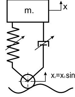
Figure 1: A single degree of freedom of quarter–car model.

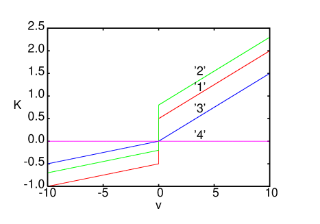
Figure 2: Damping term $K$ against velocity for $\alpha=0.5$ and $k_{1}=0.1$, $k_{2}=0.5$, $\Delta k=0.0$ for ’1’; $k_{1}=0.1$, $k_{2}=0.5$, $\Delta k=0.3$ for ’2’; $k_{1}=0.1$, $k_{2}=0.0$, $\Delta k=0.0$ for ’3’; $k_{1}=0.0$, $k_{2}=0.0$, $\Delta k=0.0$ for ’4’.

2 The model

The dimensionless equation of motion for a single degree of freedom oscillator frequently used in description of a quarter-car model [6]

$$\ddot{x}+K(\dot{x})+x=\omega^{2}x_{0}\sin\omega t,$$ (1)

where $-K(\dot{x})$ is a damping force and $\omega^{2}x_{0}\sin\omega t$ is a kinematic excitation term dependent on the vehicle speed and the roughness of the road surface. For simplicity we assumed that this surface can be described by a harmonic function (Eq. 1).

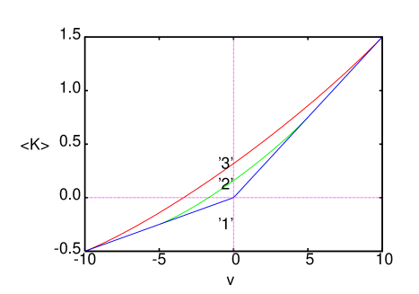
Figure 3: Averaged damping term $<K>$ against velocity $v$ where $k_{1}=0.1$, $k_{2}=0.5$, $\Delta k=0.0$ for ’1’; $k_{1}=0.1$, $k_{2}=0.5$, $\Delta k=0.3$ for ’2’; $k_{1}=0.1$, $k_{2}=0.0$, $\Delta k=0.0$ for ’3’(as in Fig. 1), and $\omega x_{0}=10$.

Here we assumed that the nonlinear damping force $-K(\dot{x})$ is of Bingham type [1, 2]

$$K(\dot{x})=k_{1}(1+\alpha{\rm sgn}\dot{x})\dot{x}+k_{2}{\rm sgn}\dot{x}+\Delta k.$$ (2)

Some examples of possible damping characteristics are presented in Fig. 2. Note, the above force term possesses singular points where the damping is non-continuous (lines ’1’,’2’) or non-smooth (line ’3’). Usually, the mirror symmetry ($v$ $\rightarrow$ $-v$) is broken by the change in slopes (line ’3’) [6]. Additionally, it can be also associated with constant term (’2’ and ’3’) related to the direction dependent dry friction phenomenon [7]. Using the above model we will investigate the effect of oscillations with high frequency. For a quarter-car model (Fig. 1) this effect could appear during its motion with high speed.

3 Calculations and Results

The large value of excitation frequency $\omega>>1$ introduces naturally to second ’fast’ time scale in our system (Fig. 1).

In fact the multiple time-scale method is an efficient and widely used treatment for nonlinear mechanical systems [8, 9, 10] to get an approximate analytic solution. In these cases the time-scales are introduced to account for nonlinear terms in the examined systems. On the other hand, the fast time scale can be introduced through excitation terms in the limit of very high excitation frequency [7, 11, 12, 13]. In various nonlinear systems [7], subjected to additional excitation fast and slow time-scales, such splitting is realized physically. It enables to estimate a behaviour in terms of the averaged system equations of motion after averaging over fast oscillations.

Note, comparing to our system (Eqs. 1,2) in the original treatment by Thomsen, $k_{1}=0$ $k_{2}\neq 0$ and $\Delta k\neq 0$ [7, 11] to describe the effect of dry friction. On the other hand, in Ref. [6] $k_{2}=0$ and $\Delta k=0$, $k_{1}\neq 0$ for a quarter-car model. Below we will consider the most general case with damping (Eq. 2) described by all nonzero terms.

Assuming that $\omega>>1$ we define second (fast) time scale by introducing a small parameter:

$$\epsilon=\omega^{-1}$$ (3)

Following Thomsen (2005) [11] we define two time scales fast given by $T_{0}$ and slow by $T_{1}$, respectively

$$T_{0}=\epsilon^{-1}t,~{}~{}~{}~{}T_{1}=t.$$ (4)

Then two corresponding time derivatives $D_{0}$ and $D_{1}$ are

$$D_{0}=\partial/\partial T_{0},~{}~{}~{}~{}~{}D_{1}=\partial/\partial T_{1}.$$ (5)

The original time derivatives can be written as follows

$$\frac{\rm d}{{\rm d}t}=\epsilon^{-1}D_{0}+D_{1},$$ (6)

$$\frac{{\rm d}^{2}}{{\rm d}t^{2}}=\epsilon^{-2}D_{0}^{2}+2\epsilon^{-1}D_{0}D_{1}+D_{1}^{2},$$

while a two component solution reads

$$x(T_{0},T_{1})=z(T_{1})+\epsilon\xi(T_{0},T_{1}).$$ (7)

By introducing the above quantities (Eqs. 4,7) into the initial equation of motion (Eq. 1) and collecting terms by $\epsilon^{-1}$ we obtain equation for a fast motion part

$$D_{0}^{2}\xi=\omega x_{0}\sin(T_{0}).$$ (8)

On the other hand for a slow motion one gets (collecting terms by $\epsilon^{0}$)

$$D_{1}^{2}z+K(D_{1}z+D_{0}\xi)+z=0.$$ (9)

To find a solution for $z$ in the last equation (Eq. 9) we have to examine fast oscillations in $\xi$ and perform averaging of the whole equation in the excitation period $2\pi$ (in the fast $T_{0}$ time scale).

At first, we get a solution for $\xi$ from Eq. 8

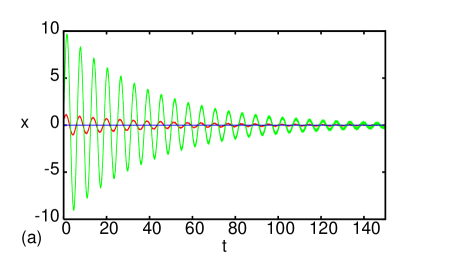
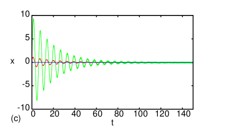
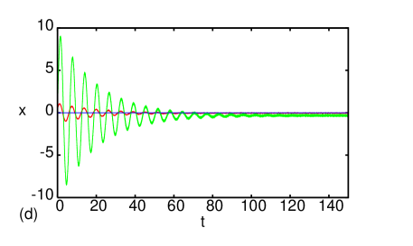
Figure 4: Time histories of damping term for system parameters: $k_{1}=0.05$, $k_{2}=0$, $\Delta k=0$, $\omega=100$ and (a) $\alpha=0.1$, (b) $\alpha=0.5$, (c) $\alpha=0.1$, (d) $\alpha=0.5$, and $x_{0}=0.01$ (red line), $x_{0}=0.1$ (green line) respectively.

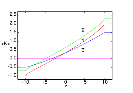
Figure 5: Averaged values of a damping term $<K>$ against velocity $v$ ($\alpha=0.5$, $k_{1}=0.1$) without excitation ’1’ and with an excitation term ’2’–’3’ for $\omega x_{0}=5$ and 10, respectively. Note the curve ’3’ may correspond to case $x_{0}=0.1$ and $\omega=100$.

$$\xi(T_{0})=-\omega x_{0}\sin(T_{0}).$$ (10)

Then averaging procedure for a damping term can be written as

$$<K(D_{1}z+D_{0}\xi)> = \frac{1}{2\pi}\int_{0}^{2\pi}\left(k_{1}(1+\alpha{\rm sgn}(D_{1}z+D_{0}\xi))(D_{1}z+D_{0}\xi)\right.$$ (11)

$$+ \left.k_{2}{\rm sgn}(D_{1}z+D_{0}\xi))+\Delta k\right){\rm d}\tau$$

By using Eq. 10 and evaluating the above integral we get

$$<K> = k_{1}\alpha\frac{1}{2\pi}\int_{0}^{2\pi}(D_{1}z-x_{0}\omega\cos\tau){\rm sgn}(D_{1}z-x_{0}\omega\cos\tau){\rm d}\tau$$ (12)

$$+ k_{2}\frac{1}{2\pi}\int_{0}^{2\pi}{\rm sgn}(D_{1}z-x_{0}\omega\cos\tau){\rm d}\tau+\Delta k,$$

where $\tau=T_{0}\in[0,2\pi]$.

After integration we get an analytical formula for the averaged damping term

$$<K> = \left[1-\frac{2}{\pi}\arccos{\left(\frac{D_{1}z}{x_{0}\omega}\right)}\right](k_{2}+k_{1}\alpha D_{1}z)$$ (13)

$$+ \frac{2}{\pi}\sin\left[\arccos{\left(\frac{D_{1}z}{x_{0}\omega}\right)}\right]k_{1}\alpha x_{0}\omega+k_{1}D_{1}z+\Delta k.$$

It is obvious that $x_{0}\omega$ is a control parameter which scaling influences averaged damping in a nontrivial way.

Following Thomsen [7, 11] discussion on dry friction, we decided to plot the results (Eq. 13) for three values of $x_{0}\omega$ and $k_{2}=0$ and $\Delta k=0$ in Fig. 3. For comparison we have also performed the simulations of the system, using Eq. 1, for large $\omega$ ($\omega=100$). Figures 4a–d show the results for different choice of system parameters. The simulation results show that the product $x_{0}\omega$ and $\alpha$ determine the effective damping. It is visible directly in envelops of quenching curves as well as in the asymptotic equilibrium value $<x>=\lim_{t\rightarrow\infty}x$. In our simulation cases Figs. 4 a–d we have got $<x>\approx$ 0, -0.02, -0.006, -0.031 for red lines; $<x>\approx$ 0, -0.2, -0.06, -0.31 for green lines. Note that the simulation result shown in Fig. 4d $<x>\approx-0.31$ (for the green line) agrees with the analytic result (Eq. 12, Fig. 3 – line ’3’). This agreement is due to the equilibrium of effective damping for $v=0$ and the static displacement force (note, the stiffness coefficient is equal to 1). Finally, in Fig. 5 we show the effective damping $<K>$ for various choices of damping terms (Eq. 2) including asymmetric friction phenomenon related to curves plotted in Fig. 2. When comparing these two figures (Figs. 2 and 5) one can observe that fast oscillations can easily eliminate the non-smoothness and discontinuities in the original characteristics. As we expected, asymmetries in the initial damping terms (Eq. 2) lead to new equilibrium point.

4 Summary and Conclusions

We have examined vibrations of a single-degree of freedom oscillator with MR fluid damper subjected to kinematic excitations. Nontrivial behaviour of the system is immanent feature of the MR fluid damper. For defined magnetic fluid characteristics [2, 6], we have used the procedure based on fast and slow scales splitting and, in this way, we have derived effective damping coefficient depending on magnetic fluid characteristics. Consequently, we have shown how the initial oscillations were quenched out in presence of fast kinematic forcing. Presence of asymmetry in the original damping terms (Eq. 2) changes the equilibrium point.

We should add that the effect of fast excitations can appear in a different way including external forcing of various kinds and an additional degree of freedom. Particularly this effect can be used to improve brake systems in cars [14].

References

- [1] B.F. Jr. Spencer, S.J. Dyke, M.K. Sain, and J.D. Carlson, ”Phenomenological model of a magnetorheological damper”, ASCE Journal of Engineering Mechanics 123 (1997) 230-238.
- [2] S.M. Savaresi, S. Bittanti, and M. Montiglio, ”Identification of semi–physical and black-box non-linear models: the case of MR-dampers for vehicles control”, Automatica 41 (2005) 113-127.
- [3] M. Borowiec, G. Litak, M.I. Friswell, ”Nonlinear response of an oscillator with a magneto-rheological damper subjected to external forcing”, Applied Mechanics and Materials 5-6 (2006) 277-284.
- [4] S. Guo, S. Yang, and C. Pan, ”Dynamic modeling of magnetorheological damper behaviors”, Journal of Intelligent Material Systems and Structures 17 (2006) 3-14.
- [5] D. Fisher and R. Isermann, ”Mechatronic semi-active vehicle suspensions”, Control Engineering Practice 12 (2004) 1353-1367.
- [6] U. von Wagner, ”On non-linear stochastic dynamics of quarter car models”, International Journal of Non-Linear Mechanics 39 (2004) 753 -765.
- [7] J.J. Thomsen, Vibrations and Stability, Springer, Berlin 2003.
- [8] A.H. Nayfeh and D.T. Mook, Nonlinear Oscillations New York: Wiley 1979.
- [9] M.P. Cartmell, S.W. Ziegler, R. Khanin, and D.I.M. Forehand, ”Multiple scales analyses of the dynamics of weakly nonlinear mechanical systems”, Applied Mechanics Reviews, 56 (2003) 455 492.
- [10] J. Warmiński, G. Litak, M.P. Cartmell, R. Khanin, and M. Wiercigroch, ”Approximate Analytical Solutions for Primary Chatter in the Non-linear Metal Cutting Model”, Journal of Sound and Vibration, 259 ( 2003) 917 933.
- [11] J.J. Thomsen, ”Slow high-frequency effects in mechanics: problems, solutions, potentials”, International Journal of Bifurcation and Chaos 9 (2005) 2799-2818.
- [12] S. Chatterjee, T.K. Singha, ”Controlling chaotic instability of cutting process by high–frequency excitation: a numerical investigation”, Journal of Sound and Vibration 267 (2003) 1184-1192.
- [13] G. Litak, R. Kasperek, K. Zaleski, ”Regenerative Metal Cutting: Effect of High-Frequency Excitation”, unpublished Computational Materials Science (2006) submitted.
- [14] J. Toon, J. Sanders, ”Stopping the noise: active control system could halt squealing brakes in cars, trucks and buses”, Georgia Institute of Technology of Technology Research News, June 16 (2003).