1/f noise and multifractality in atmospheric-CO₂ records

Abstract

We study the fluctuations in the measured atmospheric CO₂ records from several stations and show that it displays $1/f$ noise and multifractality. Using detrended fluctuation analysis and wavelet based methods, we estimate the scaling exponents at various time scales. We also simulate CO₂ time series from an atmospheric chemistry-transport model (CTM) and show that eventhough the model results are in broad agreement with the measured exponents there are still some discrepancies between them. The implications for sources and sinks inversion of atmospheric-CO₂ is discussed.

Atmospheric carbon dioxide is thought to be one of the greenhouse gases primarily responsible for the current phase of global warming co2 . In view of this significance for the global climate and life on earth, considerable effort has gone into measuring CO₂ from various platforms in the last several decades. Direct record of atmospheric CO₂ is available since the 1950s and hourly time series are constructed more recently at several measurement stations co2ts ; data . In the context of atmospheric systems, where the mean behaviour is reasonably well known from such long term records, the fluctuations decide the actual outcome. However, the fluctuation properties of CO₂ time series have not been studied in sufficient detail. Such a study would help identify the class of process, e.g, correlated random walk, Levy flight etc., underlying the CO₂ biogeochemistry and will provide a clue if it is a self-organised critical system. Secondly, this would serve as a diagnostic tool to compare the outputs from ab initio atmospheric CTMs as well as to constrain the processes that could be represented in them. This could lead to better understanding of the global CO₂ cycle.

Scale invariance and $1/f$ noise are considered to be the signatures of complex systems complex . In recent years, several time series from physiological, economic, physical systems including those of atmospheric parameters have been subjected to scaling and spectral analysis dfa1 . If $x(t)$ be the given time series, then the scaling can be expressed as, $x(\alpha t)\approx\alpha^{H}x(t)$, where the symbol $\approx$ denotes statistical equality and the the scaling exponent $H$ is also called the Hurst exponent. In many of naturally occuring phenomena, a suitable measure of their fluctuations $F(L)$ displays a power law as a function of length $L$ of the time series, i.e, $F(L)\propto L^{H}$. Physically this implies that if $0<H<1$ then they are long range correlated. In particular, $H=1/2$ corresponds to white noise and $H=1$ to $1/f$ noise. A suitable stochastic model of long range correlations is the fractional Brownian motion (fBm) dfa1 . Significantly, many natural processes such as the temperature and precipitation (as also many economic and physiological time series) behave like a fBm process and exhibit long range correlation with a exponent that is claimed to be universal in some of those cases. For instance, in the case of temperature fluctuations at inland sites far from the oceans the exponent is $H\approx 0.65$ temp1 . See also Ref temp2 for a debate. Similar analysis of rainfall has been used to suggest that rain events might be a case of self-organised criticality (SOC) rain . Infact, the idea that many natural processes might display $1/f$ noise and SOC-like behaviour btw is one of the impetus for this line of research. However, to the best of our knowledge, the fluctuation properties of the chemical species in the atmosphere such as CO₂ have not been studied. In this letter, we examine the experimentally measured high frequency (hourly) CO₂ time series from 28 stations and show that their flucuations display a power law with $H\approx 1$ corresponding to $f^{-\beta}$ ($\beta\approx 1$) noise at intermediate frequencies. We also simultaneously examine the model simulations of atmospheric-CO₂ and discuss its implications.

The measured CO₂ concentrations constitute a non-stationary time series and hence we apply the detrended fluctuation analysis (DFA) dfa2 to quantify the fluctuations and its behaviour in the spectral domain. An alternative approach is to use wavelets wlet of appropriate basis such that it allows for separation between high and low frequency components through successive levels of decomposition. We will only briefly mention the techniques here since both the methods are widely reported in the literature dfa2 ; wlet . We denote by $x(k)$ the CO₂ concentration in parts per million (ppm) measured at discrete times $k=1,2,....k_{max}$. The corresponding integrated series given by, $y(t)=\sum_{k=1}^{t}x(k)$, $t=1,2....k_{max}$. The detrending is done by dividing the series $y(t)$ into $M$ segments each containing $\tau$ data points and by empirically fitting a linear, quadratic, cubic … function $\tilde{y}(t)$ to each of them. Then, the fluctuations about the fitted trend in each of the segment is obtained as,

$$F(\tau)=\sqrt{\frac{1}{\tau}\sum_{t=1}^{k_{max}}(y(t)-\tilde{y}(t))^{2}}.$$ (1)

The fluctuations $F(\tau)$ averaged over all the $M$ segments of size $\tau$ is denoted by $\langle F(\tau)\rangle$. In many cases, $\langle F(\tau)\rangle\propto\tau^{H}$. In the case of standard random walk, $H=3/2$. Note that the exponent $H$ is related to the power spectral exponent of $x(k)$ through $\beta=2H-1$ and to its fractal dimension $D=2-H$ dfa1 . We also obtain the fluctuation function $F(\tau)$ using Daubechies wavelet wlet , an orthogonal wavelet family with largest number of vanishing wavelet coefficients. We perform 9 levels of wavelet decomposition corresponding to quadratic detrending.

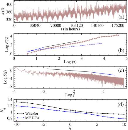
Figure 1: (a) Hourly time series of measured CO₂ concentration at Brotjacklriegel, Germany. (b) DFA applied to this time series (solid dots) shows two distinct time scales with different scaling exponents. The blue line is the best fit line with slope of 1.440 $\pm$ 0.012. The black line fits the second region with slope of 0.953 $\pm$ 0.011. The dashed line is the shuffled data and has a slope of 0.517, close to that of white noise. (c) The power spectrum of CO₂ series displays corresponding distinct frequency scaling. The blue line is obtained as the best fit one with slope -1.920 $\pm$ 0.023 and the black line has the slope of -1.080 $\pm$ 0.032. The latter region displays low-frequency $1/f$ noise. (d) Plot of $H_{q}$ against $q$ as a signature of multifractality.

The hourly CO₂ data are available in the public domain for 28 stations, some of which have long period of measurements going as far back as 1972 data . As a typical case, Fig 1(a) displays the time series of CO₂ concentrations in ppm obtained at Brotjacklriegel, Germany. Apart from the hourly fluctuations, the profile shows an approximate periodicity of about one year which is related to the consumption pattern of CO₂ by the vegetation in the northern hemisphere. In Fig 1(b), we show the result of DFA performed on this data. Two distinct scaling regimes can be identified. For a time scale of few hours to two weeks, denoted by blue line in Fig 1(b), we obtain a best fit slope of 1.440 and this closely corresponds to 3/2 one gets for a random walk process. For a time scale of about 30 days (shown as black line), the estimated slope is 0.953 and this regime closely corresponds to $1/f$ noise. At longer time scales beyond $\tau>300$ days, we see an approximate white noise like behaviour with $H\approx 0.512$. In order verify that these correlations are genuine, we create a surrogate by randomly shuffling the series while retaining the same distribution. Random shuffling would kill the correlations present in the data. The DFA performed on this shuffled surrogate data (shown as a dashed line) has a slope of 0.517, in close agreement with the white noise exponent of 0.5. We have also verified the DFA exponents using the wavelet decomposition as well. The power spectrum in Fig 1(c) displays, as expected based on DFA results, $1/f$ noise at intermediate frequencies (black line) and $1/f^{2}$ behaviour at higher frequencies (blue line). Notice that the estimated exponents $H$ in Fig 1(b) are related to the power spectral exponents $\beta$ in Fig 1(c) through $\beta=2H-1$. The results in Fig 1(c) also indicate that at low frequencies the spectrum is approximately flat representative of white noise. This succession of three different regimes in the power spectrum corresponding to white noise ($f^{0}$) at low, 1/f noise ($f^{-1}$) at intermediate and random walk ($f^{-2}$) at high frequencies can be generated from a superposition of exponential relaxation processes of the type $N(t)=N_{0}\exp(-\lambda t)$ with the uniform distribution $g(\lambda)$ of relaxation rates $\lambda$ relax . While it might be tempting to suggest this as a model for atmospheric-CO₂ variability, further work needs to be done both at the level of statistics and much more in terms of CO₂ science to understand the modeling aspect further. Further, we will present results to show that this scaling behaviour is generic to hourly CO₂ data from all the stations, with the notable exception of Samoa and South Pole.

As shown above, Fig 1(b) displays atleast three distinct scaling regimes which indicates the possibility that CO₂ time series could be a multifractal. In a monofractal, all the moments of the fluctuations have the same scaling exponent $H$. For a multifractal, $q$th moment is given by,

$$F(\tau)=\left(\frac{1}{\tau}\sum_{t=1}^{k_{max}}(y(t)-\tilde{y}(t))^{q}\right)^{1/q}\propto\tau^{H_{q}}$$ (2)

and the exponents $H_{q}$ are dependent on order $q$. We compute $H_{q}$ using multifractal-DFA (MFDFA) and wavelet formalism mfdfa and in Fig 1(d), we show $H_{q}$ plotted against $q$. Note that at $q=2$, we have $H_{2}=1.062$, in close agreement with $H$ obtained using DFA and wavelet methods earlier. We will show that CO₂ series from all the stations display multifractal characteristics.

Our aim in rest of the study is to show that the scaling results presented in Fig. 1 are generic to almost all the sites for which the data is available. For this purpose, we consider the following 8 stations station chosen to represent various geophysical features; namely, Waldhof (LGB), Schauinsland (SSL) both in Germany, Ryori (RYO), Hateruma (HAT) both in Japan, Barrow (BRW) in the USA, Jubany (JBN) in Argentina, Puszeza Borecka (DIG) in Poland and Anmyeon-do (AMY) in Republic of Korea. We show the DFA fluctuation functions for these stations in Fig 2(a). In all the cases, atleast two distinct scaling regimes are visible; the blue line represents the random walk type scaling regime while the black line represents the $1/f$ noise type scaling. The mean dfa exponent for these stations in the former regime is $H\approx 1.404\pm 0.125$ while for the latter it is $H\approx 0.978\pm 0.087$ closely approximating unity necessary for $1/f$ noise. The power spectrum shown in Fig 2(b) provides a direct evidence of this. Beyond this, at longer time scales of about 130 days ($\log\tau>3.5$), some of the stations, AMY for instance, display white noise type scaling as indicated by the dashed line. However, the white noise regime does not seem to exist in all the stations. In order to obtain a global picture, the histogram of DFA exponents for all the stations is shown in Fig 3. Note that most of the exponents assume a value between 0.8 and 1.1 which is our central result that intermediate frequency CO₂ series exhibits $1/f$ noise. The power spectrum of these stations (not shown here) also confirms the $1/f$ scaling. In Fig 3(b), the histogram of $H$ for short time scales of less than 14 days ($1/f^{2}$ regime) is shown. Most of the exponents lie within the range 1.3-1.7, in close vicinity of 1.5 needed for $1/f^{2}$ type power spectrum.

Thus, Figs 2 and 3 taken together reveal $1/f$ noise (indicated as black line) for a time scale of approximately 30 - 50 days in high frequency CO₂ records and it joins the host of other phenomena that display $1/f$ behaviour complex . Performing similar analysis on the daily averaged data (not shown here) shows up $1/f$ noise on similar time scales.

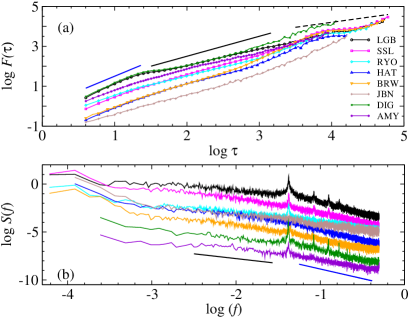
Figure 2: (a) Fluctuation function $F(\tau)$ shown in log-log plot for seven stations. Atleast two distinct scaling regions can be seen. Blue line has a slope of 1.5 and the black line has a slope of 1 meant for comparison purposes. (b) Power spectrum for the same set of stations as in (a) in the same order in which the station name appears in the legend. $y$-axis values are shifted for clarity. The slope of black line is -1 and that of blue line is -2, both meant for comparison with the power spectrum of actual data.

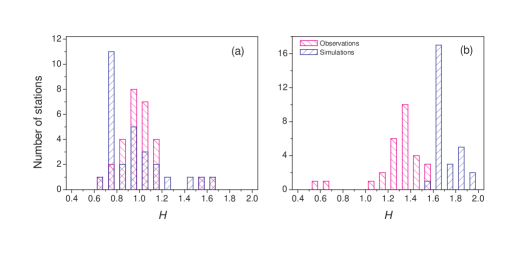
Figure 3: Histogram of DFA exponents for all the 28 stations, using both model simulations (blue) and observations (magenta). (a) shows exponents from $1/f$ region and (b) shows exponents from $1/f^{2}$ exponents (see text for details).

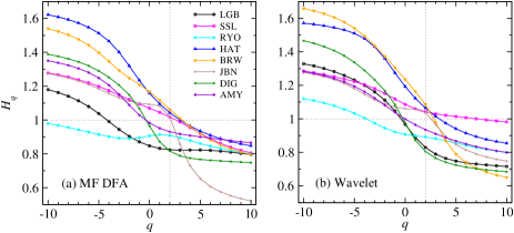
Figure 4: Dimension spectrum as a signature of multifractality at intermediate frequencies ($1/f$ regime at $q=2$) for the same set of stations shown in Fig 2. At $q=2$, most of the stations have $H_{2}\approx 1$.

The theoretical modelling of CO₂ fluxes is presently an important activity and it reflects the current understanding of global CO₂ cycle model . In order to compare our observation based results against a theoretical benchmark, we perform scaling analysis using DFA on the time series obtained from atmospheric CTM. We simulate the atmospheric-CO₂ time series using a transport model and prescribed surface fluxes due to oceanic exchange (monthly), terrestrial biosphere (3-hourly) and annual mean fossil fuel emission model1 . The transport model is based on the CCSR/NIES/FRCGC atmospheric general circulation model (AGCM) nudgged with NCEP-FNL analysed wind vectors and temperature model2 . The AGCM includes transport of chemical constituents due to advection, convection, and turbulent mixing processes. The model is run at T106 ($\sim$1.125$\times$1.125) horizontal resolutions and 32 vertical layers for the period 2002-2003 following a spin-up of 2 years. The DFA exponents obtained from the CO₂ time series simulated by the model at hourly time interval are shown in Fig. 3. Most of the model simulated exponents lie within the bins 0.7-1.2 (shown as blue line) though about half of them assume values in the range of 0.7 to 0.8. The overlap between the two histograms in Fig 3(a) shows an overall broad agreement along with the differences in details that reflects partly the modelling deficiencies. For instance, it is known that the correlation between the measured CO₂ fluxes and the simulated ones for seasonal time scales (corresponding partly to $1/f$ scaling regime) is 0.8 or greater model . The histograms for the $f^{-2}$ random walk type regime in Fig 3(b) shows that even more discrepancies exist between measured and model results. This is because the synoptic scale ($\sim$7-10 days) variations in CO₂ are not reproduced by the model simulations (correlation 0.5 or smaller) model . With this short period of simulation experiment, namely 2 years, it is not possible to observe the white noise regime.

The results presented above are generic for most of the stations except remote sites like Samoa and South Pole. Significant deviations are observed mainly in the $f^{-2}$ regime at remote observation sites, roughly in proportion to the distance from the regions of fastest CO₂ exchange, namely the forested lands and countries with greater human activity. For instance, the large deviations between the scaling exponents from modelled and observed time series are seen for the periods until 2, 7, 8 and 74 days at Izana, Samoa, Mauna Loa and South Pole, respectively.

This comparison results suggest that the transport and flux models are fairly realistic over the region of fast and large CO₂ exchanges at the surface. But further studies are required to understand the behaviour of CO₂ variations at the remote sites like Samoa and South Pole. Both these stations display significant deviations from the scaling results presented above. We believe, such information can be used as a diagnostic tool for testing the terrestrial and ocean ecosystem flux model results as appropriate. In sources and sinks inversion of atmospheric-CO₂, the forward model simulation lengths of basis functions and presubtracted fluxes are dictated by the flux memory in CO₂ time series enting . Thus such scaling analysis would help in defining the forward simulation lengths and the time scale of future flux inversion studies.

Further, we show that multifractality is generic to CO₂ time series. We calculate $H_{q}$ for the observed data at stations shown in Fig 4 using MFDFA and wavelet formalism. We stress that the results from multifractal-DFA mfdfa and wavelets are quantitatively similar. The MFDFA results from modelled CO₂ time series also exhibit multifractality, though they do not agree quantitatively with the observation based results. This once again suggests that the models are picking up broadly the correct behaviour in atmospheric-CO₂ but missing out the details.

We have studied the scaling properties of high-frequency atmospheric-CO₂ time series at 28 stations around the globe. At intermediate time scales of about a month, CO₂ data exhibits $1/f$ noise. At shorter time scales of about a week, we get $1/f^{2}$ noise. We also show that the CO₂ series is a multifractal implying that manty different time scales are present in the system. We also examine the ab initio atmospheric chemistry model outputs and show that the model results reasonably reproduce the statistical properties of the measured series. The implications of these results in estimation and analysis of surface fluxes are discussed.

- (1) Climate Change 2001: The Scientific Basis, J. T. Houghton et. al. (eds), (Cambridge University Press, Cambridge, 2002).
- (2) C. D. Keeling et. al., Tellus 28(6), 538 (1976).
- (3) Available for 28 stations at http://gaw.kishou.go.jp. See also Green house gases and other atmospheric gases, volume IV, WMO/GAW/WDCGG No. 30, Japan Meteorological Agency, Tokyo, Japan (2006).
- (4) H. J. Jensen, Self-organised criticality; Emergent Complex Behaviour in Physical and Biological Systems, (Cambridge University Press, UK, 1998).
- (5) Fractals and chaos in geology and geophysics, D. L. Turcotte, (Cambridge University Press, Cambridge, 1997); Science of Disasters : Climate disruptions, heart attacks and market crashes, edited by A. Bunde, J. Kropp and H.J. Schnellhuber, (Springer, Berlin, 2002); S. Havlin et. al., Physica A, 273, 46 (1999); M. Ausloos, Physica A bf 336, 93 (2004).
- (6) Eva Koscielny-Bunde et. al., Phys. Rev. Lett. 81 729 (1998); K. Freadrich and R. Blender, Phys. Rev. Lett. 90, 108501 (2003).
- (7) A. Bunde et. al.,, Phys. Rev. Lett. 92 039801 (2004); K. Freadrich et. al.,, Phys. Rev. Lett. 92 039802 (2004).
- (8) Ole Peters and K. Christensen, Phys. Rev. E 66, 036120 (2002); Jan W. Kantelhardt et. al., J. Geophys. Res. 111, D01106 (2006).
- (9) P. Bak, C. Tang and K. Wiesenfeld, Phys. Rev. Lett. 59, 381 (1987); P. Bak and K. Chen, Sci. Am. 79 46 (1991).
- (10) C-K. Peng et. al.,, Phys. Rev. E 49, 1685 (1994); Zhi Chen et. al.,, Phys. Rev. E 65, 041107 (2002).
- (11) I. Daubechies, Ten Lectures on wavelets, SIAM, Philadelphia (1992); P. Manimaran et. al.,, J. Phys. A 39, L599 (2006).
- (12) E. Milotti, Phys. Rev. E 72, 056701 (2005); B. Kaulakys et. al.,, Phys. Rev. E 71, 051105 (2005).
- (13) J. W. Kantelhardt et. al.,, Physica A 316, 87 (2002).
- (14) Apart from these 8 stations, the other 20 that form the basis for this study are DEU, NGL, SCH, WST, ZGT all in Germany; COI, DDR, KIS, MKW, MNM, TKY, YON in Japan; Mauna Loa, Samoa in USA; Izana in Spain; FDT in Romania; PAL in Finland and SNB in Austria and South Pole (see data for details).
- (15) C. Geels et. al., Tellus B 56(1), 35 (2004); P. K. Patra et. al., Atmos. Chem. Phys. Discuss. 6, 6801 (2006); R. M. Law et. al., in preparation.
- (16) T. Takahashi et. al., Deep-sea Res. II 49, 1601 (2002); S. C. Olsen and J. T. Randerson, J. Geophys. Res. 109, D02301 (2004); A. L. Brenkert, Carbon Dioxide Information Analysis Center, ORNL, Oak Ridge (2003).
- (17) A. Numaguti, M. Takahashi, T. Nakajima, A Sumi, CGER’s Supercomput. Monogr. Rep. I-3, Tsukuba (1997); M. Takigawa et. al., J. Geophys. Res. 110, D21313 (2005).
- (18) I. G. Enting, Inverse Problems in Atmospheric Constituent Transport, (Cambridge Univ. Press, Cambridge, 2002).