Local excitation-lateral inhibition interaction yields wave instabilities in spatial systems involving finite propagation delay

Abstract

The work studies wave activity in spatial systems, which exhibit nonlocal spatial interactions at the presence of a finite propagation speed. We find analytically propagation delay-induced wave instabilities for various local excitatory and lateral inhibitory spatial interactions. The final numerical simulation confirms the analytical results.

1 Introduction

In the recent decades the space-time dynamics of extended complex systems has attracted much attention in physical, chemical and biological science [7, 17]. In this context the nonlocal interactions between system subunits have been studied extensively [3, 16, 24]. By virtue of this nonlocal spatial interaction, the propagation delay between two spatial locations may not be negligible if the the propagation speed in the system is small enough. Such propagation delays have been found to affect the activity spread solids [4, 13] and plasmas [5], they affect the stability of neuronal systems [10] or may be responsible for subballistic transport in solids [22]. The present work addresses these phenomena and studies the effect of a finite propagation speed in a generic spatio-temporal model.
To describe the space-time evolution of nonlocal systems mathematically, partial differential equations have been studied vastly, e.g. [8, 17]. Moreover integral-differential equations also have been studied in recent years to describe nonlocal interaction in spatially extended neuronal systems [2, 3, 18, 19, 24]. Both latter equation types are strongly related for some specific integral-differential equations [11, 1]. To illustrate this relation, assume a one-dimensional spatial field $u(x)$ and the spatial kernel function $K(x)$. Then it is

$$\int_{-\infty}^{\infty}K(x-y)u(y)dy=\int_{-\infty}^{\infty}\tilde{K}(k)\tilde{u}(k)e^{ikx}dk$$

with the Fourier transforms $\tilde{K}$ and $\tilde{u}$ of $K$ and $u$, respectively. Then choosing $K(x)=\exp(-|x|/\sqrt{D})/2\sqrt{D}$, it is $\tilde{K}(k)=1/(1+Dk^{2})=1-Dk^{2}+D^{2}k^{4}+\cdots$ and Eq. (1) reads

$$\int_{-\infty}^{\infty}K(x-y)u(y)dy \approx u(x,t)+D\Delta u(x,t)$$

$$+D^{2}\Delta^{2}u(x,t)+\cdots$$

with $\Delta=\partial^{2}/\partial x^{2}$. This means that fast-decaying integral kernels $K(x)$ with $\sqrt{D}\ll 1$ represents a local diffusion process with diffusion constant $D$, while slowly-decaying integral kernels yield higher orders of spatial derivatives and thus represent long-ranged or nonlocal interactions. This procedure has been studied in some more detail in a previous work [1] and it turned out that integral-differential equations generalize some types of partial differential equations. In this context the present work extends the previous work by the study of a more general spatio-temporal model.
In the research field of spatially extended systems, let the underlying model be partial differential equations or integral-differential equations, it is well-known that local excitation and lateral inhibition (local inhibition and lateral excitation) may yield stationary (non-stationary) spatial patterns in one or more spatial dimensions [16, 10]. However, a recent study showed that local inhibition and lateral excitation may yield stationary instabilities as well for gamma-stributed spatial interactions [1]. This finding let us look more carefully on the nature of spatial interactions and the classification criteria for these instabilities. The present work investigates wether there are traveling waves in local excitatory and lateral inhibitory systems, which may contrast to the findings in previous studies.
The work is structured as follows. The subsequent section introduces and motivates the generic model studied and presents the steps of corresponding linear stability analysis about a stationar state. Then section 3 applies the model to a field of harmonically damped oscillators, which are coupled by nonlocal excitation and inhibition. The analytically results are confirmed by numerical simulations. The subsequent summary closes the work.

2 The generic model

The model studied presumes identical elements which obey the (non-)linear differential equation

$$\hat{T}_{t}V(x,t) = h[V(x,t)]~{}.$$

Here $V(x,t)$ represents the scalar activity variable, $\hat{T}_{t}=\hat{T}_{t}(\partial/\partial t)$ denotes the temporal operator and the functional $h[V(x,t)]$ defines the local dynamics at spatial location $x$. Let the elements $\{x\}$ be located in a spatial domain and coupled to each other. This configuration reflects a topological network with identical elements in which no spatial metric is considered, or a topological network embedded in a physical space [25, 12]. In the the present model the single elements are connected according to a probability density function similar to topological networks but their connectivity function depend on the Euclidean distance between the elements similar to spatial networks. Further the spatial coupling is presumed homogeneous in space, that is the coupling is dependent on the spatial distance between the elements. These properties describe a scale-free lattice [14, 21]. Moreover, the presented model presumes infinitely dense elements, that is we consider a continuous field. This contrasts to networks whose major element is the discreteness. However in biological systems, e.g. in the brain, the single cells are dense and the continuum limit holds [23]. Furthermore the speed by which the activity is transmitted between single elements shall be finite. This finite propagation speed also contrasts to most spatial networks, which frequently neglect propagation delay effects.

Considering all previous aspects, the element at spatial location $x$ obeys the integral-differential equation

$$\hat{T}_{t}V(x,t) = h[V(x,t)]+I(x,t)$$

$$+\int_{\Omega}K(x-y)f\left[V(y,t-\frac{|x-y|}{v_{K}})\right]$$

$$+L(x-y)g\left[V(y,t-\frac{|x-y|}{v_{L}})\right]~{}dy.$$

Here $I(x,t)$ represents the external input and the kernel functions $K,~{}L$ represent the probability density functions of spatial connections in two networks, and thus $K(x)$ and $L(x)$ are normalized to unity in the spatial domain $\Omega$. In the following we assume $\Omega={\mathcal{R}}$. The functionals $f[V]$ and $g[V]$ represent the (non-)linear coupling functions. Further the model considers propagation delays between spatial locations $x$ and $y$ at distance $|x-y|$ due to the finite transmission speed $v_{K}$ and $v_{L}$ corresponding to the two networks. This model allows the study of a wide range of combined spatial interaction. For instance spatial systems involving both mean-field and local interactions may be modeled by $K(x)=const$ and $L(x)=\delta(x)$, respectively. The subsequent paragraphs focus on the combination of excitatory and inhibitory interactions with kernel functions $K(x)$ and $L(x)$, respectively. In addition we specify $f[V]=a_{K}S[V],~{}g[V]=a_{L}S[V]$ with the nonlinear functional $S[V]$ and the total amount of excitation and inhibition $a_{K}$ and $a_{L}$, respectively. Further we presume $a_{K}>a_{L}$. For $h(V)=0$, Eq. (2) represents a well-studied nonlocal model of neural populations [20, 3, 10, 1, 9].

First let us determine the stationary state which is constant in space and time. Applying a constant external input $I_{0}$, we find the implicit equation $0=h(V_{0})+f(V_{0})+g(V_{0})+I_{0}$. Here we used the fact that the kernel functions are normalized to unity. Then small deviations $u(x,t)$ about the stationary state obey a linear evolution equation and relax in time to the stationary state $V_{0}$ with $u(x,t)\sim e^{\lambda t},~{}\lambda\in~{}{\mathcal{C}}$ if $Re(\lambda)<0$. Then the subsequent expansion of $u(x,t)$ in the continuous Fourier basis $\{e^{ikz}\}$ yields the implicit condition

$$T(\lambda)=h_{0}+S^{\prime}\int_{\Omega}dy\,$$

$$\times\left(a_{K}K(y)e^{-\lambda|y|/v_{K}}-a_{L}L(y)e^{-\lambda|y|/v_{L}}\right)e^{iky}$$

(1)

with $h_{0}=\partial h/\partial V$, $S^{\prime}=\partial S/\partial V$ computed at $V=V_{0}$. Since the external input drives the system, its stability is subjected to $I_{0}$ and subsequently $S^{\prime}$ represents the reasonable control parameter. Equation (1) is difficult to solve exactly for $\lambda$. In a previous study a more specific model has been studied in detail for stationary and non-stationary instabilities [1]. We follow its approach and consider large but finite propagation speeds. Then it is $\exp(-\lambda|z|/v)\approx 1-(\lambda/v)|z|$ for $|\lambda|/v_{K},~{}|\lambda_{L}|/v_{L}\ll 1$ and (1) reads

$$T(\lambda)\approx h_{0}+S^{\prime}\tilde{K}_{0}(k)-\lambda S^{\prime}\tilde{K}_{1}(k)~{}.$$ (2)

with

$$\tilde{K}_{0}(k) = a_{K}\tilde{K}^{(0)}(k)-a_{L}\tilde{L}^{(0)}(k)$$

$$\tilde{K}_{1}(k) =\frac{a_{K}}{v_{K}}\tilde{K}^{(1)}(k)-\frac{a_{L}}{v_{L}}\tilde{L}^{(1)}(k)$$

with $\tilde{F}^{(n)}(k)=\int_{-\infty}^{\infty}F(z)|z|^{n}\exp(-ikz)dz$. The term $\tilde{K}_{0}(k)$ and $\tilde{K}_{1}(k)$ represents the Fourier transform and the first kernel Fourier moment of $a_{K}K(x)+a_{L}L(x)$, respectively. Essentially let us specify the temporal evolution of a single element to a damped oscillator with

$$\hat{T}_{t}=\frac{\partial^{2}}{\partial t^{2}}+\gamma\frac{\partial}{\partial t}+1.$$

Then the stability threshold of stationary and non-stationary instabilities read

$$\frac{1}{S^{\prime}_{c}} = \frac{\tilde{K}_{0}(k_{c})}{1-h_{0}}\quad\mbox{(stationary instability)}$$ (3)

$$\frac{1}{S^{\prime}_{c}} = -\frac{\tilde{K}_{1}(k)}{\gamma}\quad\mbox{(non-stationary instability)}$$

Hence the global maximum of $\tilde{K}_{0}(k_{c})$ and $-\tilde{K}_{1}(k_{c})$ define the critical wavenumber $k_{c}$ and the critical threshold $S^{\prime}_{c}$ of stationary and non-stationary instabilities, respectively. Figure 1 illustrates this result for non-stationary instabilities. In the following, we call an emerging non-stationary phenomena a wave instability, if $k_{c}\neq 0$. and the instability with $k_{c}=0$ is called a global oscillation. Moreover it is interesting to note that the threshold of the non-stationary instability does not depend on the local (non-)linear dynamics of the elements $h(V)$.

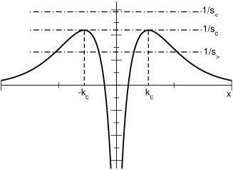
Figure 1: Sketch to illustrate the mechanism of non-stationary instabilities. The plot shows the right hand side of Eq. (LABEL:eqn_k) (solid line) and its left hand side (dot-dashed line). If the stability threshold is not reached, i.e. $S^{\prime}=s_{<}<S^{\prime}_{c}$, the system is stable. In contrast, if $S^{\prime}=s_{c}=S^{\prime}_{c}$ ($S^{\prime}=s_{>}>S^{\prime}_{c}$) the system is marginal stable (unstable).

3 Application to specific model

First let us discuss briefly various types of nonlocal interactions. We choose the excitatory and inhibitory spatial kernel to the gamma function and the decreasing exponential function, resp., with

$$K(z)=\frac{1}{2q^{p}\Gamma(p)}|z|^{p-1}e^{-|z|/q}~{},~{}L(z)=\frac{1}{2r}e^{-|z|/r}~{}$$ (5)

Since the Eq. (LABEL:eqn_k) does not depend on $h[V]$, we set $h[V]=0$. In other words, the single elements in the field are assumed damped harmonic oscillators, which are coupled by an excitatory and an inhibitory network. The parameter $r$ defines the spatial range of the inhibitory interaction, while both $p$ and $q$ represent the spatial constants of the excitatory nonlocal interaction. The scase $p=1$ is well-studied, see e.g. [10], and the combination of $q$ and $r$ yield the four important cases, namely the global excitation, the global inhibition, the local excitation-lateral inhibition and the local inhibition-lateral excitation. Further the choice $p>1$ yields local inhibitory interactions or local inhibitory-lateral excitatory interactions [1]. The present work focus on the case $p<1$ which yields the local excitation or the local excitation-lateral inhibition. Please see Fig. 2 for the corresponding illustration of the cases $p<1$ and $p>1$.

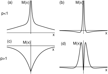
Figure 2: Illustration for some spatial interaction types for different parameters $p,q$ and $r$. Panel (a) shows the kernel function for $p<1,~{}q>r$ that yields global excitations while panel (b) reveals local excitation-lateral inhibition for $p<1,~{}q<r$. In panel (c) the kernel function has been illustrated for $p>1,~{}q<r$, which represents global inhibition, while panel (d) shows local inhibition-lateral excitation for $p>1,~{}q>r$. It is $M(x)=K(x)-L(x)$

In order to gain the critical wavenumber of the wave instability, the kernel Fourier moment in Eq. (LABEL:eqn_k) is computed to

$$\tilde{K}^{(1)}(k) = \frac{pq\cos((p+1)\arctan(kq))}{(1+q^{2}k^{2})^{(p+1)/2}}$$ (6)

$$\tilde{L}^{(1)}(k) = \frac{r\cos(2\arctan(kr))}{(1+r^{2}k^{2})}$$ (7)

Since $\tilde{K}_{1}(k)\to 0$ for $|k|\to\infty$, there is a maximum of $-\tilde{K}_{1}(k)$ at some $|k|=|k_{c}|$ with $-\tilde{K}_{1}(k_{c})>0$ if $-\tilde{K}_{1}(0)>0$ and $-d^{2}\tilde{K}_{1}(0)/dk^{2}>0$. These sufficient conditions read

$$\xi>p/a_{r}~{},~{}\xi^{3}<\frac{v_{r}}{6a_{r}}p(p+1)(p+2)$$ (8)

with the new parameters $\xi=r/q,~{}v_{r}=v_{L}/v_{K}$ and $a_{r}=a_{L}/a_{K}<1$.

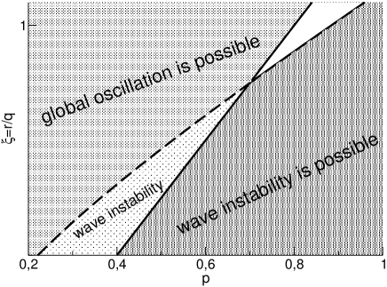
Figure 3: The occurrence of oscillatory instabilities subject to the parameters $\xi=r/q$ and $p$. The dashed and thin solid line represent the function $\xi=(v_{r}p(p+1)(p+2)/6a_{r})^{1/3}$ and $\xi=p/a_{r}$, respectively, taken from Eq. (8). Here it is $v_{r}=1,~{}a_{r}=0.8$ .

Figure 3 illustrates the different parameter regimes of the conditions. At first it turns out that there is large parameter regime which allows for non-stationary instabilities. In order to gain further insight to the nature of spatial interactions for $p<1$, Fig. 4 shows the parameter regimes and the different number of roots of the kernel function $K(z)$. We find a parameter regime of single roots, which reflects local excitation-lateral inhibition interaction, and a parameter regime of no roots, i.e. global excitation. Moreover, there is a parameter regime of multiple roots which, for instance, reflects local excitation - mid-range inhibition - lateral excitation and allows for wave instabilities.

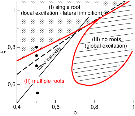
Figure 4: Number of zero-croosings, i.e. roots, of the kernel function $K(z)$ and the corresponding nature of spatial interactions subject to the parameters $\xi$ and $p$. The dashed and thin solid line are taken from Fig. 3. The red lines delimits the novel parameter regime of multiple roots. In addition to the parameters from Fig. 3, it is $a_{K}=10,~{}a_{L}=8,v_{K}=v_{L}=1$ and $q=1$.

To illustrate the relation of the spatial interaction type and the resulting non-stationary instability, Figure 5 plots the kernel functions $K(z)$ and the corresponding negative first kernel Fourier moments $-\tilde{K}_{1}(k)$ for four different cases of spatial interactions. These specific cases are denoted by filled dots in Fig. 4. We find local excitation-lateral inhibition for $\xi=0.8$ (top row, left panel in Fig. 4). Since the global maximum of $-\tilde{K}_{1}(k)$ gives the critical wavenumber $k_{c}$, this case yields global oscillations with $k_{c}=0$ (top row, right panel in Fig. 4). For $\xi=0.75$, now the kernel function exhibits two roots which still leads to global oscillations. In case of $\xi=0.70$ the sufficient condition for wave instabilities are fulfilled, as $-\tilde{K}_{1}(k)$ reveals a critical wavenumber $k_{c}\neq 0$, see Fig. 4. Moreover, the spatial interaction function reveals local excitation, mid-range inhibition and lateral excitation, which has not been found yet in previous studies. At last for $\xi=0.55$ there is also a wave instability showing local excitation, mid-range inhibition and lateral excitation.

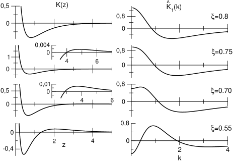
Figure 5: The kernel functions $a_{K}K(z)+a_{L}L(z)$ and the negative first kernel Fourier moment $\tilde{K}_{1}(k)$ for the four different cases taken from Fig. 4. The insets in the left coloumn represent foci of the corresponding plot to illustrate the additional lateral excitation. The parameters are taken from Fig. 4 and the different values of $\xi$ correspond to the different dots in Fig. 4.

In addition to this study, Fig. 6 compares the spatial interaction function, the Fourier transform $\tilde{K}_{0}$ and $-\tilde{K}_{1}(k)$ for two values of $\xi$. This comparison is necessary as the stationary instability may occur first before the wave instability while increasing the control parameter from small values. For both parameter values of $\xi$ the global maximum of $-\tilde{K}_{1}(k)$ exceeds the global maximum of $\tilde{K}_{0}$ and thus a wave instability and not a stationary instability may occur. Thus Fig. 6 supports the previous findings.

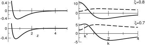
Figure 6: The comparison of the kernel functions $a_{K}K(z)+a_{L}L(z)$ (left coloumn), the Fourier transform $\tilde{K}_{0}(k)$ (dashed line in right coloumn) and $-\tilde{K}_{1}(k)$ (solid line in right coloumn) for two values of $\xi$. Additional parameters are taken from Fig. 4.

To visualize and confirm the analytical findings, finally we integrate the integral-differential equation  (2) numerically. The Euler integration scheme is applied for the time evolution integration and the Monte-Carlo method VEGAS  [15, 6] computed the spatial integration. This specific Monte-Carlo integration method combines stratified and importance sampling, which is important to gain good estimates of the divergent excitatory kernel function. Moreover boundary conditions are set periodic with the period $L$ while the initial conditions have to be defined in the time interval $t_{0}\in[-L/v;0]$. We have chosen $V(z,t_{0})=\cos(k_{c}x)+0.5*\cos(5k_{c}x)$.

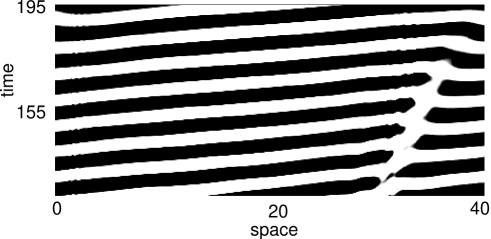
Figure 7: Space-time plot of the integrated activity for $p=0.5,~{}r=0.7$ shows the wave instability for local excitation - lateral inhibition interactions. Additional parameters are $a_{K}=10,~{}a_{L}=8,~{}v_{K}=v_{L}=0.6,~{}\gamma=0.2,~{}I_{0}=2.8,~{}dx=0.089,~{}dt=0.08$ and $h[V]=0,~{}S[V]=1/(1+\exp(-1.84(V-3.0)))$. These parameters yields $k_{c}=0.4$.

Figure 7 shows the wave instability for $p=0.5,~{}\xi=0.7$ discussed above, cf. Fig. 4, and confirms the analytical finding.

4 Summary

The present work describes the nonlocal spatial interaction of single elements in a continuous field. The application to damped oscillators, which are coupled by both nonlocal excitation and inhibition, reveals a new mechanism of wave instabilities. In contrast to previous findings in pattern forming systems, we find wave instabilities for local excitation and lateral inhibition. To obtain more information on the corresponding spatial interaction, we investigated additionally the spatial interaction function. It turns out that various spatial interaction types exhibit wave instabilities, as local excitation-lateral inhibition and local excitation-midrange inhibition-lateral excitation. Hence the sign of the spatial interaction function does not carry the full information of the expected instability patterns in spatial systems with finite propagation delay. We have observed that the comparison of the global maximum of the Fourier component and global maximum of the negative first kernel Fourier moment allows for a reliable estimation of the instability type.
Future work shall study the classifiers in vectorial models, as the nonlocal version of the Bruesselator, and the classification scheme in two- and three-dimensional systems.

Appendix: The kernel Fourier moments

The n-th kernel Fourier moment of the specific kernels (5) can be computed from

$$I(p) = \int_{0}^{\infty}x^{p-1}e^{-z/q}\cos(kx)\,dx$$

$$= \Gamma(p)\left(\frac{1}{q^{2}}+k^{2}\right)^{-p/2}\cos\left(p\arctan(kq)\right)$$

Then we find for the excitatory kernel

$$\tilde{K}^{(n)}(k) = \frac{1}{q^{p}\Gamma(p)}~{}I(p+n)$$

$$= \frac{\Gamma(p+n)}{\Gamma(p)}\frac{q^{n}\cos\left((p+n)\arctan(kq)\right)}{(1+q^{2}k^{2})^{(p+n)/2}}~{}.$$

In addition, we find

$$-\frac{\partial^{2}}{\partial k^{2}}\tilde{K}^{(n)}(k)=\tilde{K}^{(n+2)}(k)~{}.$$

Since the inhibitory kernel is a specific case of the excitatory kernel with $p=1$ and $q=r$, we obtain Eqs. (6), (7) from the previous expressions.

References

- [1] A.Hutt and F.M.Atay. Analysis of nonlocal neural fields for both general and gamma-distributed connectivities. Physica D, 203:30–54, 2005.
- [2] A.Hutt and F.M.Atay. Effects of distributed transmission speeds on propagating activity in neural populations. Phys. Rev. E, 73:021906, 2006.
- [3] S. Coombes. Waves and bumps in neural field theories. Biological Cybernetics, 93:91–108, 2005.
- [4] D.Y.Tzou and J.K.Chen. Thermal lagging in random media. J. Thermophys. Heat Transfer, 12:567–574, 1998.
- [5] E.Lazzaro and H.Wilhelmsson. Fast heat pulse propagation in hot plasmas. Physics of plasmas, 5(4):2830–2835, 1998.
- [6] B. Gough. GNU Scientific Library Reference Manual. Network Theory Ltd, 2 edition, 2003.
- [7] H. Haken. Brain Dynamics. Springer, Berlin, 2002.
- [8] H. Haken. Synergetics: Introduction and Advanced topics. Springer, Berlin, 2004.
- [9] A. Hutt. Effects of nonlocal feedback on traveling fronts in neural fields subject to transmission delay. Phys. Rev. E, 70:052902, 2004.
- [10] A. Hutt, M. Bestehorn, and T. Wennekers. Pattern formation in intracortical neuronal fields. Network: Comput. Neural Syst., 14:351–368, 2003.
- [11] J.D.Murray. Mathematical Biology. Springer, Berlin, 1989.
- [12] J. Jost and J.M. Joy. Evolving networks with distance preferences. Phys. Rev. E, 66:036126, 2002.
- [13] K.Mitra, S.Kumar, A.Vedavarz, and M.K.Moallemi. Experimental evidence of hyperbolic heat conduction in processed meat. ASME J. Heat Transfer, 117:568–573, 1995.
- [14] K.Yang, L.Huang, and L.Yang. Lattice scale-free networks with weighted linking. Phys.Rev.E, 70:015102, 2004.
- [15] G.P. Lepage. A new algorithm for adaptive multidimensional integration. J. Comput. Phys., 27:192–203, 1978.
- [16] M.C.Cross and P.C.Hohenberg. Pattern formation outside of equilibrium. Reviews of Modern Physics, 65(3):851–1114, 1993.
- [17] G. Nicolis and I. Prigogine. Self-Organization in Non-Equilibrium Systems: From Dissipative Structures to Order Through Fluctuations. J. Wiley and Sons, New York, 1977.
- [18] P.Blomquist, J.Wyller, and G.T.Einevoll. Localized activity patterns in two-population neuronal networks. Physica D, 206:180–212, 2005.
- [19] P.C.Bressloff. Synaptically generated wave propagation in excitable neural media. Phys. Rev. Lett., 82(14):2979–2982, 1999.
- [20] D.J. Pinto and G.B Ermentrout. Spatially structured activity in synaptically coupled neuronal networks: I. travelling fronts and pulses. SIAM J. Applied Math., 62(1):206–225, 2001.
- [21] R.Karmakar and S.S.Manna. Sandpile model on an optimized scale-free network on euclidean space. J. Phys. A: Math. Gen., 38:L87–L93, 2005.
- [22] R.Metzler and T.F.Nonnenmacher. Fractional diffusion, waiting-time distributions, and cattaneo-type equations. Phys.Rev.E, 57:6409–6414, 1998.
- [23] J.L. van Hemmen. Continuum limit of discrete neuronal structures: is cortical tissue an ’excitable’ medium? Biol. Cybern., 91(6):347–358, 2004.
- [24] H.R. Wilson and J.D. Cowan. Excitatory and inhibitory interactions in localized populations of model neurons. Biophys. J., 12:1–24, 1972.
- [25] R. Xulvi-Brunet and I.M. Sokolov. Evolving networks with disadvantaged long-range connections. Phys. Rev. E, 66:026118, 2002.