Whitham method for Benjamin-Ono-Burgers equation and dispersive shocks in internal waves in deep fluid

Abstract

The Whitham modulation equations for the parameters of a periodic solution are derived using the generalized Lagrangian approach for the case of damped Benjamin-Ono equation. The structure of the dispersive shock in internal wave in deep water is considered by this method.

I Introduction

As is known, dispersive shock is an oscillatory structure generated in wave systems after wave breaking of intensive pulse under condition that the dispersive effects are much greater than the dissipative ones. In this sense, such shocks are dispersive counterparts of usual viscous shocks well known in dynamics of compressive viscous fluids. In the surface water waves physics, the dispersive shocks are known as tidal bores in rivers BL . Besides this classical observation, the dispersive shocks have been also found in some other physical systems including plasma plasma and Bose-Einstein condensate simula ; hoefer .

In typical situations, a dispersive shock can be represented as a modulated nonlinear wave whose parameters change little in one wavelength and one period; hence the Whitham modulation theory whitham1 ; whitham2 (see also kamch2000 ) can be applied to its study. If one neglects dissipation, then dispersive shock is a non-stationary structure expanding with time so that at one its edge it can be represented as a soliton train and at the other edge as a linear wave propagating with some group velocity into the unperturbed region. A corresponding Whitham theory of such shocks for the systems described by the Korteweg-de Vries (KdV) equation was developed by Gurevich and Pitaevskii in GP1 and later it was extended to other equations such as the Kaup-Boussinesq system egp ; egk1 , Benjamin-Ono (BO) equation matsuno1 ; matsuno2 ; jorge , and nonlinear Schrödinger equation kku . This approach has found applications to water waves physics apel and dynamics of Bose-Einstein condensate kgk1 ; hoefer .

The Whitham method describes a long time evolution of the dispersive shock when many waves (crests) are generated. However, when the long-time evolution is considered, the small dissipation effects can become of crucial importance. In particular, they can stop self-similar expansion of the shock so that it tends to some stationary wave structure which propagates as a whole with constant velocity. Correspondingly, the Whitham equations should be modified to include the dissipation effects. For the first time it was done for the KdV-Burgers equation in gp2 ; akn by direct method which did not use applicability of the inverse scattering transform method to the KdV equation. More general approach based on the complete integrability of unperturbed wave equations was developed in kamch04 and applied to the theory of bores described by the Kaup-Boussinesq-Burgers equation egk2 and the KdV equation with Chezy friction and a bottom with a slope egk3 .

The method of Ref. kamch04 can be applied in principle to any wave equation which is completely integrable in framework of the AKNS method akns and any perturbation depending on the wave variables and their space derivatives. However, the important BO equation describing internal waves in stratified deep water includes the non-local dispersion term and therefore it cannot be considered by the method of kamch04 . Although the Whitham theory for the BO was discussed in matsuno1 ; matsuno2 ; jorge ; dk , its generalization to taking into account small dispersion effects has not been developed yet. The aim of this paper is to develop the Whitham theory for the Benjamin-Ono-Burgers equation

$$u_{t}+uu_{x}+Hu_{xx}=\varepsilon u_{xx},$$ (1)

where

$$Hu(x)=\frac{1}{\pi}\mathrm{P.V.}\int\frac{u(y)}{y-x}dy$$ (2)

is the Hilbert transform and the term in the right-hand side of (1) describes small friction with the viscosity parameter $\epsilon$. In the next Section we shall derive the Whitham equations which govern slow evolution of the nonlinear periodic wave due to its modulation and small friction and in Section III we shall apply this theory to the stationary bore (dispersive shock).

II Whitham theory for the Benjamin-Ono-Burgers equation

The unperturbed BO equation has a periodic solution

$$u(x,t)=\frac{4k^{2}}{\sqrt{A^{2}+4k^{2}}-A\cos\theta}+\beta,\quad\theta=kx-\omega t,$$ (3)

which depends on three constant parameters—wavenumber $k$, amplitude of oscillations $A=(u_{max}-u_{min})/2$, and $\beta$. This solution describes a nonlinear wave propagating with constant velocity

$$V=\frac{\omega}{k}=\frac{1}{2}\sqrt{A^{2}+4k^{2}}+\beta.$$ (4)

In a modulated wave these three parameters become slow functions of the space and time coordinates and their evolution is governed by the Whitham equations which were obtained in dk for the general multi-phase solutions of the unperturbed BO equation by the method based on the complete integrability of the BO equation and in matsuno1 ; matsuno2 for the simplest one-phase solution (3) by a direct Whitham method based on the use of the Hamilton principle

$$\delta\int dt\int dxL(\phi,\phi_{x},\phi_{t})=0$$ (5)

with the Lagrangian

$$L=\frac{1}{2}\phi_{t}\phi_{x}+\frac{1}{6}\phi_{x}^{3}+\frac{1}{2}\phi_{x}H\phi_{xx},\quad u=\phi_{x}.$$ (6)

In this method the periodic solution is represented in the form

$$\phi=\psi+\Phi(\theta),$$ (7)

where

$$\psi=\beta x-\gamma t,\quad\theta=kx-\omega t,$$ (8)

so that

$$\beta=\psi_{x},\quad\gamma=-\psi_{t},\quad k=\theta_{x},\quad\omega=-\theta_{t};$$ (9)

hence $u=u(\theta,\theta_{x},\theta_{t},\psi_{x})$, $L=L(\theta,\theta_{x},\theta_{t},\psi_{x},\psi_{t})$, and the averaging is taken over fast oscillations according to the rule

$$\overline{L}=\frac{1}{2\pi}\int_{0}^{2\pi}Ld\theta$$ (10)

leading to the averaged Lagrangian which depends on the derivatives $\theta_{x},\theta_{t},\psi_{x},\psi_{t}$. The Euler-Lagrange equations for the corresponding averaged Hamilton principle

$$\delta\int dt\int dx\overline{L}(\theta_{x},\theta_{t},\psi_{x},\psi_{t})=0$$ (11)

yields with account of (9) the Whitham equations in the form

$$\frac{\partial}{\partial t}\frac{\partial\overline{L}}{\partial\gamma}-\frac{\partial}{\partial x}\frac{\partial\overline{L}}{\partial\beta}=0,\quad\frac{\partial}{\partial t}\frac{\partial\overline{L}}{\partial\omega}-\frac{\partial}{\partial x}\frac{\partial\overline{L}}{\partial k}=0,$$ (12)

which should be complemented by the consistency conditions

$$\beta_{x}+\gamma_{t}=0,\quad k_{t}+\omega_{x}=0.$$ (13)

After calculation of the integral (10) they reduce to the system of equations for the parameters $\beta,k,V=\omega/k$ (see matsuno1 ; matsuno2 ).

Now our task is to generalize this procedure to the perturbed BO equation (1). Instead of using the Lagrangian formulation with an additional field (see, for instance, Ref. KaupMalomed ) we prefer to introduce a more simple approach which does not require introduction of new auxiliary fields. We propose to use directly the Hamilton principle in its infinitesimal form by noticing that Eq. (1) can be written symbolically as

$$\int dt\int dx\left\{\delta L+\varepsilon\phi_{xxx}\delta\phi\right\}=0,$$ (14)

where $\delta L$ is a variation of the Lagrangian (6). Now we can transform (14) in the following way. First, we integrate the “dissipative” term by parts and use $u=\phi_{x}$:

$$\int dt\int dx\left\{\delta L-\varepsilon u_{x}\delta u\right\}=0.$$ (15)

Second, we average the dissipative term as follows:

$$\begin{split}\int dx\overline{(u_{x}\delta u)}=\int dx\overline{[u_{x}(u_{\theta}\delta\theta+u_{\theta_{x}}\delta\theta_{x}+u_{\theta_{t}}\delta\theta_{t}+u_{\psi_{x}}\delta\psi_{x})]}\\ =\int dx\left\{\overline{\left[u_{x}u_{\theta}-\frac{\partial}{\partial x}(u_{x}u_{\theta_{x}})-\frac{\partial}{\partial t}(u_{x}u_{\theta_{t}})\right]}\delta\theta-\frac{\partial}{\partial x}\overline{(u_{x}u_{\psi_{x}})}\delta\psi\right\}.\end{split}$$

In the Whitham approximation with fast $\theta$-variable we have $\partial/\partial x\cong\theta_{x}\partial/\partial\theta$, $\partial/\partial t\cong\theta_{t}\partial/\partial\theta$, where within the averaging interval the parameters $\theta_{x}$ and $\theta_{t}$ can be considered constant, the terms with $\theta$-derivatives become equal to zero after averaging and, hence, we arrive at the expression

$$\int dt\int dx\overline{(u_{x}\delta u)}=\int dt\int dx\overline{(u_{x}u_{\theta})}\delta\theta=\int dt\int dxk\overline{(u_{\theta}^{2})}\delta\theta.$$ (16)

Transformation of the term with Lagrangian in (15) can be performed in a similar way and as a result we obtain the Whitham equations in the form

$$\frac{\partial}{\partial t}\frac{\partial\overline{L}}{\partial\gamma}-\frac{\partial}{\partial x}\frac{\partial\overline{L}}{\partial\beta}=0,\quad\frac{\partial}{\partial t}\frac{\partial\overline{L}}{\partial\omega}-\frac{\partial}{\partial x}\frac{\partial\overline{L}}{\partial k}=\varepsilon k\overline{(u_{\theta}^{2})},$$ (17)

which generalize Eqs. (12) to the BOB equation (1).

Simple calculation of averaged values gives matsuno1 ; matsuno2

$$\overline{L}=\frac{1}{3}k^{3}-k\left(\frac{\omega^{2}}{k^{2}}-\frac{\beta\omega}{k}+\gamma\right)+\frac{1}{6}\beta^{3}-\frac{1}{2}\beta\gamma,$$ (18)

$$\varepsilon k\overline{(u_{\theta}^{2})}=2\varepsilon(V-\beta)[(V-\beta)^{2}-k^{2}].$$ (19)

Their substitution into (17) and use of (13) permit one to express $\gamma$ as $\gamma=\beta^{2}/2$ and transform equations for the other parameters to the form

$$\begin{split}&\beta_{t}+\beta\beta_{x}=0,\\ &k_{t}+(Vk)_{x}=0,\\ &V_{t}+VV_{x}+kk_{x}=-\varepsilon(V-\beta)[(V-\beta)^{2}-k^{2}].\end{split}$$ (20)

These are the Whitham equations for the physical parameters $\beta,k,V$.

Although equations (20) are simple enough for further investigations, they can be transformed to theoretically more attractive diagonal form by introduction of Riemann invariants $a,b,c$ according to definitions

$$\beta=2c,\quad k=b-a,\quad V=b+a,\quad(c<a<b),$$ (21)

so that we get the system

$$\begin{split}&a_{t}+2aa_{x}=-2\varepsilon(a-c)(b-c)(a+b-2c),\\ &b_{t}+2bb_{x}=-2\varepsilon(a-c)(b-c)(a+b-2c),\\ &c_{t}+2cc_{x}=0.\end{split}$$ (22)

In terms of Riemann invariants the periodic solution (3) takes the form

$$u(x,t)=\frac{2(b-a)^{2}}{a+b-2c-2\sqrt{(a-c)(b-c)}\,\cos\theta}+2c,$$ (23)

where

$$\theta=(b-a)x-(b^{2}-a^{2})t.$$ (24)

The parameters $a,b,c$ must satisfy the condition $2c<a+b$ to keep the solution non-singular. The amplitude of oscillations is expressed as

$$A=4\sqrt{(a-c)(b-c)}.$$ (25)

When for some concrete problem the solution of Eqs. (22) is found and the functions $a=a(x,t),$ $b=b(x,t),$ $c=c(x,t)$ are known, their substitution into (23) yields the modulated nonlinear wave for the problem under consideration. Mean value of $u$ in this oscillatory region is equal to

$$\overline{u}=2k+\beta=2(b+c-a).$$ (26)

In the next Section we shall consider an example of such a problem.

III Dispersive shock (bore) in internal waves in a deep fluid

As was mentioned in the Introduction, the dispersive shock is an oscillatory region joining two regions with different values of the wave amplitude $u_{\pm}$ which arise after wave breaking. In the simplest case of the Gurevich-Pitaevskii problem one can consider $u_{\pm}$ as two constants: $u\to u_{\pm}$ as $x\to\pm\infty$, respectively, and without loss of generality we can take $u_{+}=0$ and denote $u_{-}=u_{0}=\mathrm{const}$. Thus, we have to find the solution of the Whitham equations which corresponds to a modulated nonlinear wave satisfying the boundary conditions

$$u\to\left\{\begin{array}[]{c}u_{0},\quad x\to-\infty,\\ 0,\quad x\to+\infty.\end{array}\right.$$ (27)

Naturally, the initial profile of the wave $u=u(x,0)$ must also satisfy this condition and easy estimate shows that after wave breaking the waves are generated with wavelength $L\sim 1/u_{0}$.

Now, we can distinguish two typical stages of evolution of the wave:

1. The initial stage for $t\ll 1/(\varepsilon u_{0}^{2})$, when we have $|u_{t}|\gg\varepsilon|u_{xx}|$, so that one can neglect a viscous term in (1);

2. The asymptotic stage of large time $t\gg 1/(\varepsilon u_{0}^{2})$, when the solution tends to the stationary solution determined by interplay of the dispersion and dissipation effects.

Examples of the first stage have already been studied in matsuno2 ; jorge . The simplest case of a step-like initial condition has been discussed in matsuno1 , and we shall reproduce some results here for convenience of future comparison with the second stage of asymptotically large time.

Thus, we suppose that at the initial moment $t=0$ the region of transition from $u=u_{0}$ to $u=0$ is very narrow (i.e. much less than $L\sim 1/u_{0}$) so that the initial profile can be approximated by a step-like function,

$$u(x,0)=\left\{\begin{array}[]{c}u_{0},\quad x<0,\\ 0,\quad x>0.\end{array}\right.$$ (28)

As was noticed above, at the initial stage we can neglect the dissipation effects, so that arising dispersive shock is governed by the equations

$$a_{t}+2aa_{x}=0,\quad b_{t}+2bb_{x}=0,\quad c_{t}+2cc_{x}=0.$$ (29)

After averaging over wavelength the initial-value problem for the Riemann invariants does not contain any parameters with dimension of length. Hence, the Riemann invariants can depend on the self-similar variable $\zeta=x/t$ only and the Whitham equations (29) reduce to

$$a_{\zeta}(2a-\zeta)=0,\quad b_{\zeta}(2b-\zeta)=0,\quad c_{\zeta}(2c-\zeta)=0.$$ (30)

Since at one edge of the oscillatory region we must have $a=b$ (the soliton limit with $k=0$) and at the other edge $a=c$ (the vanishing amplitude of oscillations limit $A=0$), the only acceptable solution of these equations reads $a=\zeta/2=x/2t$, $b=\mathrm{const},$ $c=\mathrm{const}$. According to (28), at the soliton limit $x=x_{+}$ $(a=b)$ the mean value $\overline{u}$ must match to the zero value at the right edge, $\overline{u}=2c=0$, hence $c=0$ everywhere. At the opposite edge $x=x_{-}=0$ the mean value must coincide with $u=u_{0}$, $\overline{u}=2b=u_{0}$, hence $b=u_{0}/2$ everywhere. Thus, we arrive at the following solution of the Whitham equations (see Fig. 1)

$$\begin{split}&a={x}/{2t},\quad 0<x<x_{+},\\ &b={u_{0}}/2,\quad x<x_{+},\\ &c=0,\quad x>x_{-}=0,\end{split}$$ (31)

where

$$x_{+}=u_{0}t.$$ (32)

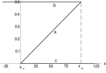
Figure 1: Plots of the Riemann invariants at $t=100$ as functions of $x$ in the case of decay of the step-like initial distribution without friction.

Substitution of this solution into (23) gives the expression for $u$ in the oscillatory region,

$$u(x,t)=\frac{(u_{0}t-x)^{2}}{t(u_{0}t+x-2\sqrt{u_{0}tx}\cos\theta)},$$ (33)

where

$$\theta=[2(u_{0}t-x)x-(u_{0}^{2}t^{2}-x^{2})]/(4t).$$ (34)

The corresponding plot of the dispersive shock profile at fixed $t$ is shown in Fig. 2.

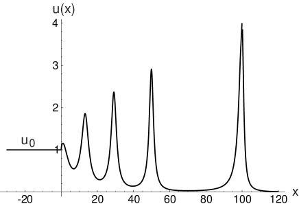
Figure 2: Profile of the bore at $t=100$ corresponding to the self-similar decay of the step-like initial distribution without friction.

At the leading front we can see a soliton with the amplitude

$$u_{s}=4V=4u_{0}$$ (35)

which moves to the right with velocity $V=u_{0}$. The trailing edge is located at $x=0$ and corresponds to a linear wave with vanishing amplitude and zero value of group velocity. Indeed, linearization of the BO equation with respect to small amplitude $A$ in $u\cong U_{0}+A\cos(kx-\omega t)$ leads to the dispersion relation

$$\omega=u_{0}k-k^{2}.$$ (36)

According to (21) we have $k=b=u_{0}/2$ at $x=0$ and hence

$$\left.\frac{d\omega}{dk}\right|_{k=u_{0}/2}=0\quad\text{at}\quad x=0.$$ (37)

Number of waves in the oscillatory region is equal to

$$N=\frac{1}{2\pi}\int_{0}^{u_{0}t}kdx=\frac{u_{0}^{2}t}{8\pi}.$$ (38)

The self-similar expansion of the oscillatory region holds as long as the viscosity effects can be neglected. However, these effects come into play at $t\sim 1/(\varepsilon u_{0}^{2})$ and at $t\to\infty$ the shock profile tends to the stationary structure propagating with constant velocity. To find this structure, we look for the stationary solution of the Whitham equations (22) so that the Riemann invariants are functions of $\xi=x-Vt$ only, where $V=a+b=\mathrm{const}$. We assume that $\xi=0$ corresponds to the leading soliton front of the shock, where $k=b-a=0$ and $\overline{u}=2(b+c-a)=0$, which give at once that $c=0$ and $a=b=V/2$ at $\xi=0$. Then the last equation (22) gives $c=0$ identically and the rest equations (22) reduce to a single equation

$$(2b-V)b_{\xi}=-2\varepsilon Vb(V-b)$$ (39)

which should be solved with the initial condition

$$\left.b\right|_{\xi=0}=\frac{V}{2}.$$ (40)

Elementary calculation with account of inequality $b>a=V-b$, i.e. $b\geq V/2$, gives at once $b=(V/2)[1+\sqrt{1-\exp(2\varepsilon V\xi)}]$. At last, at $\xi\to-\infty$ we must have $a=0$, $b=V$, $\overline{u}=u_{0}=2b=2V$, that is $V=u_{0}/2$, and we arrive at the solution

$$a=\frac{u_{0}}{4}\left[1-\sqrt{1-\exp(2\varepsilon V\xi)}\right],\quad b=\frac{u_{0}}{4}\left[1+\sqrt{1-\exp(2\varepsilon V\xi)}\right],\quad c=0,$$ (41)

where $\xi=x-(u_{0}/2)t$. Plots of the Riemann invariants are shown in Fig. 3; they should be compared with Fig. 1.

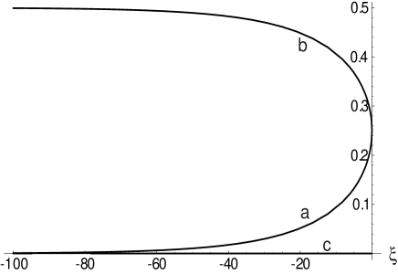
Figure 3: Plots of the Riemann invariants as functions of $\xi$ in the case of stationary bore solution with friction ($\varepsilon=0.05$).

Substitution of Eq. (41) into Eq. (23) yields the profile of the shock,

$$u(x,t)=\frac{u_{0}[1-\exp(\varepsilon u_{0}\xi)]}{1-\exp(\varepsilon u_{0}\xi/2)\,\cos\theta}$$ (42)

where

$$\theta=\frac{u_{0}}{2}\sqrt{1-\exp(\varepsilon u_{0}\xi)}\,\xi,\quad\xi=x-\frac{u_{0}}{2}t.$$ (43)

The corresponding plot is shown in Fig. 4.

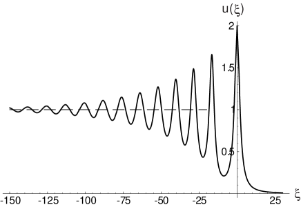
Figure 4: Profile of the stationary bore described by the Bebjamin-Ono-Burgers equation with friction coefficient $\varepsilon=0.05$. Dashed line corresponds to the constant value of $u$ at $x\to-\infty$.

Again at the leading front we can see a soliton, but now it has the amplitude

$$u_{s}=2u_{0}$$ (44)

and propagates with velocity $V=u_{0}/2$. Thus, the friction effects lead to decrease of the amplitude and velocity of the soliton compared with the non-stationary stage. However, it is important to notice that, on the contrary to an isolated soliton, the profile of the bore becomes asymptotically stationary. In this stationary solution the trailing edge is located at $x=-\infty$.

IV Conclusion

In this paper, we have discussed the structure of dispersive shock in the internal wave subject to small friction effects. It is shown that there exists a stationary profile so that non-stationary oscillating structure supported by a jump of the wave amplitudes at two spatial infinities tends asymptotically to this stationary profile.

The Whitham method applied to this problem occurs very simple in the case of BOB equation and the corresponding equations can be solved in elementary and explicit form.

References

- (1) B. Benjamin and M.J. Lighthill, Proc. R. Soc. London, Ser. A 224, 448 460 (1954).
- (2) M. Khan, S. Ghosh, S. Sarkar, and M.R. Gupta, Physica Scripta, T 116, 53 56 (2005).
- (3) T.P. Simula, P. Engels, I. Coddington, V. Schweikhard, E.A. Cornell, and R.J. Ballagh, Phys. Rev. Lett. 94, 080404 (2005).
- (4) M.A. Hoefer, M.J. Ablowitz, I. Coddington, E.A. Cornell, P. Engels, V. Schweikhard, Phys. Rev. A 74, 023623 (2006).
- (5) G.B. Whitham, Proc. Roy. Soc. London, 283, 238 (1965).
- (6) G.B. Whitham, Linear and Nonlinear Waves, (Wiley-Interscience, New York, 1974).
- (7) A.M. Kamchatnov, Nonlinear Periodic Waves and Their Modulations—An Introductory Course, (World Scientific, Singapore, 2000).
- (8) A.V. Gurevich and L.P. Pitaevskii, Zh. Eksp. Teor. Fiz., 65, 590 (1973) [Sov. Phys. JETP, 38, 291 (1973)].
- (9) G.A. El, R.H.J. Grimshaw, M.V. Pavlov, Stud. Appl. Math. 106, 157 (2001).
- (10) G.A. El, R.H.J. Grimshaw, A.M. Kamchatnov, Stud. Appl. Math. 114, 395 (2005).
- (11) Y. Matsuno, J. Phys. Soc. Japan, 67, 1814 (1998).
- (12) Y. Matsuno, Phys. Rev. E 58, 7934 (1998).
- (13) M.C. Jorge, A.A. Minzoni, N.F. Smyth, Physica D 132, 1 (1999).
- (14) A.M. Kamchatnov, R.A. Kraenkel, and B.A. Umarov, Phys. Rev. E 66, 036609 (2002).
- (15) J.P. Apel, Journ. Phys. Oceanogr. 33, 2247 (2003).
- (16) A.M. Kamchatnov, A. Gammal, and R. A. Kraenkel, Phys. Rev. A 69, 063605 (2004).
- (17) A.V. Gurevich and L.P. Pitaevskii, Sov. Phys. JETP 66, 490 (1987).
- (18) V.V. Avilov, I.M. Krichever, and S.P. Novikov, Sov. Phys. Dokl., 32, 564 (1987).
- (19) A.M. Kamchatnov, Physica, D 188, 247 261 (2004).
- (20) G.A. El, R.H.J. Grimshaw, A.M. Kamchatnov, Chaos, 15, 037102 (2005).
- (21) G.A. El, R.H.J. Grimshaw, A.M. Kamchatnov, Evolution of solitary waves and undular bores in shallow-water flows over a gradual slope with bottom friction (in preparation).
- (22) M.J. Ablowitz, D.J. Kaup, A.C. Newell, H. Segur, Stud. Appl. Math. 53, 249 (1974).
- (23) S.Yu. Dobrokhotov, I.M. Krichever, Matem. Zametki, 49, 42 (1991).
- (24) D.J. Kaup and B.A. Malomed, Phys. D 87, 155 (1995)