Stochastic description of the deterministic Ricker’s population model.

Abstract

We adopt the ’0-1’ test for chaos using Brownian motion chains to identify the dynamics of the Ricker’s population model. In the ’0-1’ test ’0’ is related to regular motion while ’1’ is associated with chaotic motion. The identified regular and chaotic types of solutions have been confirmed by means of recurrence plots.

,

The Ricker’s model [1] has been invented to analyze the population of fish. Originally the model used for stock assessment to learn and predict the population of fish and to estimate how many fish can be caught without impacting future production of fish. The dynamics of population change is given by the following map [1]:

$$x_{n+1}=F(x_{n}),~{}~{}~{}~{}F(x_{n})=Ax_{n}\exp(-x_{n}),$$ (1)

where $x_{n}$ means the population of consecutive fish generations and the constant $\mu$ depends on biological conditions, $F(x_{n})$ is a discrete transform function. A similar model has been also used in the analysis of insect data by Moran [2]. This simple model give complex answer for different system parameters. It has attracted researchers interested in emerging the chaotic solutions in mathematical biology [3]. Recently, it has been also analyzed in presence of periodic or noisy forcing [4, 5].

In this paper we will apply Eq. (1) to generate the time series of fish generations which can be latter analyzed by nonlinear stochastic methods. The corresponding transform functions $F(x_{n})$ for chosen values of the control parameter $\mu$ ($\mu=8$, 12 18.5 and 20) are plotted in Fig. 1.

We started examination of the dynamics of the above model with the time histories simulated for above chosen (Fig. 1) $\mu$ values. The time histories are presented in Fig. 2a-d. First three figures Figs. 2a-c correspond to periodic solutions with two (Figs. 2a-b) or four points (Fig. 2c). The last figure (Fig. 2d) represents a chaotic solution. Note that the steady state for periodic solutions is reached after few initial iteration points.

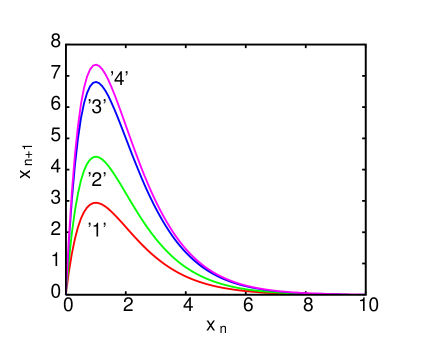
Figure 1: Transform function $F(x_{n})$ (Eq. 1). ’1’ denotes the curve for $\mu=8$ while ’2’-’4’; $\mu=12$, 18.5 and 20, respectively.

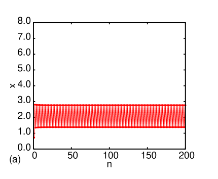
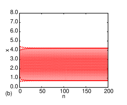
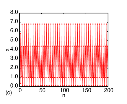
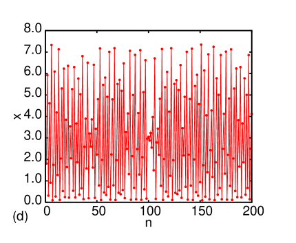
Figure 2: Time histories of $x_{n}$ (a-d) for $\mu=8$, 12, 18.5 and 20, respectively. The initial point was set to $x_{1}=0.1$.

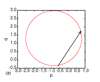
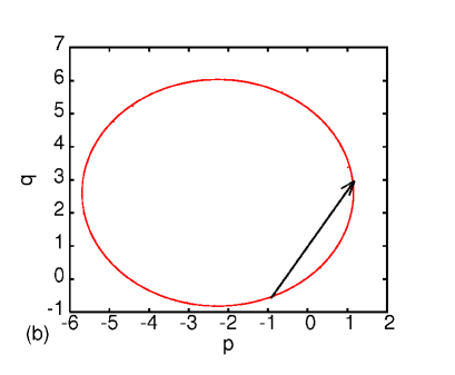
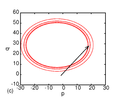
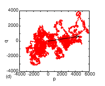
Figure 3: ’Phase portrait’ in $p-q$ coordinates. Here $p(n)$,$q(n)$ have been calculated for $n=1,...,4000000$. Arrows show the total displacement from the first to last points. The first point was set by assuming $x_{1}=0.1$. Note the scale in each figure is different.

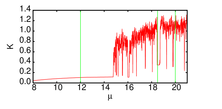
Figure 4: $K$ versus $\mu$. Vertical straight lines correspond to $\mu=8$, 12, 18.5 and 20 respectively.

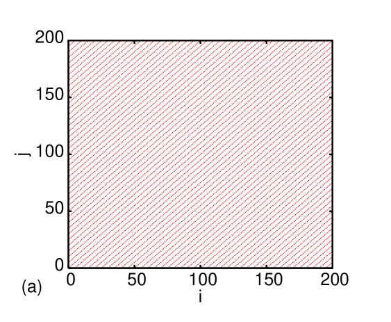
Figure 5: Recurrence plots of $x_{n}$ (a-b) for $\mu=18.5$ and 20 respectively.

Naturally the standard way to classify the dynamics of nonlinear time series is to perform reconstruction of phase space [6] and calculate the Lyapunov exponent [7, 8]. Alternatively one can adopt of ’0-1’ test method introduced by Gottwald and Melbourne [9]. The method was previously successfully tested for the Van der Pol system, the Kortweg-de Vries equations [9] the logistic map, and the Lorenz 96 system, including the system with weak noise [10].

Let us rearrange the $x_{n}$ series in the following way:

$$p(n)=\sum_{j=1}^{n}x_{j}\cos(jc),$$ (2)

for consecutive $n=1$, 2, 3, … . Here the constant $c=3.7$ has been chosen arbitrary as in Ref. [9, 10].

Note that we build new series of $p(n)$ (Eq. 4) starting with an essentially bounded coordinate $x_{n}$. However, the new series can be either bounded or unbounded depending on dynamics of the examined process: regular or chaotic, respectively. In fact for a random noise $\Gamma_{n}$ we have a Brownian motion analogy [11, 12, 13]:

$$p(n+1)=p(n)+\Gamma_{n}~{}~{}~{}n=1,2,...,N$$ (3)

Here $p(n)$ represents unbounded time series where total displacement is scaled by the square root of steps number $N$ [11]. $\Gamma_{n}$ is a diffusion term which couples different states $n\neq m$. In our case this term is given by the formula [9, 10]:

$$\Gamma_{n}=x_{n}\cos(nc).$$ (4)

Needless to say, in case of chaotic time series $x_{n}$, $\Gamma_{n}$ will mimic random behaviour [12, 13] leading to an unbounded displacement.

On the other hand for a periodic solution $x_{n}$:

$$\{x_{n}\}\rightarrow x_{1},...,x_{r},x_{1},...,x_{r},x_{1},...,x_{s},~{}~{}~{}~{}~{}{\rm for}~{}~{}~{}s<r,$$ (5)

where the index $r$ is related to a $r$-element period included in $x_{n}$ series. If it appears $j$ times in the total time series $x_{n}$ then $n=rj+s$. The parameter $p(n)$ can be expressed as (see Appendix A):

$$p(n)=p(jr+s)=\sum_{j=1}^{n}x_{j}\cos(jc)\approx-\sum_{k=1}^{r+\Theta(s-k)}x_{k}R_{nr}\sin(kc+\phi(n_{r})),$$ (6)

where $\phi(n_{r})$ and $R_{nr}$ is the angle a characteristic circle radius (Eq. LABEL:eqA.11, here $R_{nr}\approx 1$) dependent on the number of repetitions of a period $x_{1},...,x_{r}$ and a value $c$ (Appendix A) and $\Theta(\cdot)$ is the Heaviside step function.

Defining the other complementary quantity $q(n)$ in the similar way:

$$q(n)=\sum_{j=1}^{n}x_{j}\sin(jc)$$ (7)

we can derive a corresponding simplified expression for a periodic series $x_{n}$ (Eq. 5) in an analogous way. Thus an appropriate expression (Appendix A) reads:

$$q(n)=q(jr+s)=\sum_{j=1}^{n}x_{j}\cos(jc)\approx\sum_{i=1}^{r+\Theta(s-i)}x_{i}R_{nr}\cos(ic+\phi).$$ (8)

Note the pair ($q,p$) defines new coordinates in the two dimensional space. Knowing that $r$ and $s$ (Eqs. 6, 8) are usually low natural numbers (see Fig. 2 $r=2$ or 4) we can conclude that one can easily see if series $p(n)$ and $q(n)$ are bounded for arbitrary large $n$. Furthermore the simple expressions Eqs. (6) and (8) determine their trajectory in a circle like shape which radius $R$ can be easily estimated as

$$R\approx r<x_{i}>.$$ (9)

In the above expression $<\cdot>$ denotes the average value while $r$ is a period of $\{x_{n}\}$ (Eq. 5). In Fig. 3 we show examples of trajectories (plotted by consecutive points) for the examined system with four values of A as in Figs. 1-2 calculated from $x_{n}$ series using Eqs. (2,7) and for $n=1,...,4000000$. Arrows show the total displacement from the first ($n=1$) to last points ($n=4000000$). Thus depending on motion type the transformed system, into $p$ and/or $q$ coordinates, their time series show the bounded or unbounded behaviour.

To classify the dynamics in a more systematic way, we have performed the next step by calculation mean square displacement of $p(n)$ [9, 10]:

$$M(n)=\lim_{N\rightarrow\infty}\frac{1}{N}\sum_{j=1}^{N}\left(p(j+n)-p(j)\right)^{2}$$ (10)

together its asymptotic behaviour of $M(n)$ estimated by the following limit [9, 10]:

$$K=\lim_{n\rightarrow\infty}\frac{\ln(M(n)+1)}{\ln n}$$ (11)

Although the limits in the above two expressions go to $\infty$, in practice, it is enough to assume

$$N=150000~{}~{}~{}{\rm and}~{}~{}~{}n=3000000$$ (12)

to get a clear distinction between regular and chaotic states. The results for $K$ versus $\mu$ are plotted in Fig. 4. It is apparent that in case of chaotic oscillations $K\approx 1$ (mainly above $\mu=14.6$) while for regular motion $K\approx 0$ (see region below $\mu=14.6$). Some variations around 0 and 1 can be explained by a finite truncation (Eq. 12). As noted by Gottwald and Melbourne [10] the choice of the parameter $c$ can be sometimes important creating resonances which should be avoided. However we have checked this possibility in our calculations and assumed it eliminates such unwanted cases. Note that there exists a sudden change of $K\approx 1$ into lower value $K\approx 0.38$ for $\mu$ about $18.5$. Looking at Fig. 2c we know that the system is periodic with a characteristic period $r=4$. It is also bounded in terms of coordinates $p(n)$ and $q(n)$ (as can be seen in Fig. 3c) but the characteristic circle radius $R$ in ($p,q$) space is relatively large (Fig. 3c, Eq. 9) comparing to other regular states (Fig. 3a-b). It is clear from Eq. 9 as $r$ is relatively large here. To show the difference between both cases $\mu=18.5$ and 20 we plotted corresponding recurrence plots defined by the scalars $p(n)$ (without embedding) [14]. Naturally the usual way is to investigate a recurrence plot in a reconstructed phase space [15]. But as has been recently shown by Thiel at al. [14] treatment without embedding gives correct estimation of dynamical invariants and various recurrence plot analysis measures can be applied [16]. Here we plot a dot an a squared matrix whose axes correspond to the $i$ and $j$ indices if only the condition

$$\|x_{i}-x_{j}\|<\epsilon$$ (13)

is full filed, where $\epsilon$ is a certain threshold value. Using this method we can again classify independently the states of the system as regular for $\mu=18.5$ (Fig. 5a) with regular patterns (continuous diagonal lines) and chaotic for $\mu=20$, where the lines patterns appear with different finite length distributed in some random way. It indicates that the system is visiting the same region of the attractor many times [15]. The length of these short diagonal lines can be related (inversely proportional) to the largest positive Lyapunov exponent $\lambda_{1}$ [17, 15].

In summary, the 0-1 test for chaos appeared to be reliable method in case of Ricker’s model. Using a certain projection of the original time series $\{x_{n}\}$ into $p(n)$ we could use the stochastic methods to analyze the asymptotic behaviour of mean square displacement (in $p(n)$) . It enabled us to classify the system dynamics directly from scalar signal without any procedure of phase space reconstruction. Like in other systems analyzed by Gottwald and Melbourne [9, 10] for chaotic changes of consecutive fish populations we observed clear oscillations around $K=1$. On the other hand in case of regular systems it is more useful if the period of repeating chain in a time series is shorter. However in longer periods ($r=4$ for $\mu=18.5$ Fig. 4) we observed $K\approx 0.38$. We hope that this disadvantage can be reduced in future by using the estimated radius $R$ (Eq. 9) in the definition of $K$. The above method seams to be very useful for analysis of experimental data as well as for simulated dynamical systems especially those having non-continuous or non-smooth vector fields [18, 19, 20].

Acknowledgements: GL would like to thank Max Planck Institute for the Physics of Complex Systems in Dresden for hospitality.

Appendix A

For a time series represented as a large multiple sequence $x_{1},...,x_{r}$

$$x_{1},...,x_{r},x_{1},...,x_{r},x_{1},...,x_{s}$$ (A.1)

$$\sum_{j=1}^{n}x_{j}\cos(jc)=\sum_{i=1}^{s}x_{i}\left(\sum_{k=1}^{n_{r}}\cos(ic+kc)\right)+\sum_{i=s}^{r}x_{i}\left(\sum_{k=1}^{n_{r}}\cos(ic+kc)\right),$$ (A.2)

where $n_{r}$ corresponds to the multiplicity of a shorter $r$-element ($x_{1},...,x_{r}$) period inside $x_{n}$ time series. Using a simple decoupling

$$\cos(ic+kc)=\cos(ic)\cos(kc)-\sin(ic)\sin(kc)$$ (A.3)

and

$$A_{nr}=\sum_{k=1}^{n_{r}}\cos(kc)$$ (A.4)

$$=\frac{\cos c-\cos c(n_{r}+1)-1+\cos c\cos c(n_{r}+1)+\sin c\sin c(n_{r}+1)}{2-2\cos c}.$$

Similarly

$$B_{nr}=\sum_{k=1}^{n_{r}}\sin(kc)$$ (A.5)

$$=\frac{-\sin c\cos c(n_{r}+1)+\cos c\sin c(n_{r}+1)+\sin c}{2-2\cos c}$$

Figure A.1 presents results $B_{nr}$ versus $A_{nr}$ for two different values of $c$ ($c=1.7$ and $c=3.7$) note that in both cases the points are lying on circles. They are however centered in different points and have different radii $R_{c}$. In case of $c=3.7$ the radius is less than 1. The centers are given by the averages taken from Eq. A.4 and A.5.

$$A_{nr0}=0.5{\rm~{}~{}~{}for~{}any~{}~{}~{}}c,$$ (A.6)

while

$$B_{nr0}=\frac{\sin c}{2-2\cos c}.$$ (A.7)

Note, using the circles representation, both expressions for $A_{nr}$ and $B_{nr}$ (Eqs. A.4 and A.5, respectively) can be now written in a compact form

$$A_{nr}=A_{nr0}+R_{c}\cos\psi(n_{r}),$$

$$B_{nr}=B_{nr0}+R_{c}\sin\psi(n_{r}).$$ (A.8)

Interestingly for $c=3.7$ we have found numerically a change of $\psi$ versus $n_{r}$ is linear

$$\psi(n_{r})\approx 0.5584n_{r}.$$ (A.9)

Using the above notation we can write

$$\sum_{j=1}^{n}x_{j}\cos(jc)=\sum_{k=1}^{r+\Theta(s-k)}x_{k}\left(A_{nr}\cos(ck)-B_{rn}\sin(kc)\right)$$

$$=\sum_{k=1}^{r+\Theta(s-k)}x_{k}R_{nr}\cos(ck+\phi(n_{r}))$$ (A.10)

where

$$\tan(\phi)=\frac{A_{nr}}{B_{nr}},~{}~{}R_{nr}=\sqrt{A_{nr}^{2}+B_{nr}^{2}},$$ (A.11)

where $\Theta(\cdot)$ is a Heaviside step function.

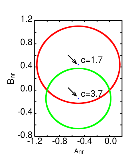
Figure 6: $B_{nr}$ versus $A_{nr}$ for $c=1.7$ and $c=3.7$, respectively. Arrows indicate corresponding circle centers.

Similar analysis can be applied for

$$\sum_{j=1}^{n}x_{j}\sin(jc)=\sum_{i=1}^{s}x_{i}\left(\sum_{k=1}^{n_{r}}\sin(ic+kc)\right)+\sum_{i=s}^{r}x_{i}\left(\sum_{k=1}^{n_{r}}\sin(ic+kc)\right),$$ (A.12)

where

$$\sin(ic+kc)=\sin(ic)\cos(kc)+\cos(ic)\sin(kc).$$ (A.13)

Therefore

$$\sum_{j=1}^{n}x_{j}\cos(jc)=\sum_{k=1}^{r+\Theta(s-k)}x_{k}\left(A_{nr}\sin(ck)+B_{rn}\sin(kc)\right)$$

$$=\sum_{k=1}^{r+\Theta(s-k)}x_{k}R_{nr}\sin(ck+\phi(n_{r})).$$ (A.14)

References

- [1] Ricker W, Stock and recruitment. Journal of the Fisheries Research Board Canada 1954;11:559–663.
- [2] Moran PAP, Some remarks on animal population dynamics. Biometrics 1950:6:250–8.
- [3] Murray JD. Mathematical biology, Springer, New York (1989).
- [4] Summers D, Cranford JG, and Healey BP. Chaos in periodically forced discrete-time ecosystem models. Chaos, Solitons & Fractals 2000:11: 2331–42.
- [5] Binder PM, Okamoto NH. Noisy integer maps. Physica A 2005: 347;51–64.
- [6] Takens, F. Detecting Strange Attractors in Tur- bulence Lecture Notes in Mathematics, Vol. 898 (Springer, Heidelberg), 1981:366–81.
- [7] Wolf A, Swift JB, Swinney HL, and Vastano JA. Determining Lyapunov exponents from a time series. Physica D 1985:16;285–317.
- [8] Kantz H. A robust method to estimate the maximal Lyapunov exponent of a time series. Phys. Lett. A 1994:185;77–87.
- [9] Gottwald GA and Melbourne I. A new test for chaos in deterministic systems. Proc R Soc Lond A 2004;460:603–11.
- [10] Gottwald GA and Melbourne I. Testing for chaos in deterministic systems with noise. Physica D 2005:212;100–10.
- [11] Risken H. The Fokker-Planck Equation. Springer Berlin 1989.
- [12] Gaspard P, Briggs ME, Francis MK, Sengers JV, Gammons RW, Dorfman JR and Calabrese RV. Experimental evidence for microscopic chaos. Nature 1998:394;865–8.
- [13] Cecconi F, Cencini M, Falcioni M, Vulpiani A. Brownian motion and diffusion: From stochastic processes to chaos and beyond Chaos 2005:15;026102.
- [14] Thiel M, Romano MC, Read PL and Kurths J. Estimation of dynamical invariants without embedding by recurrence plots. Chaos 2004:14;234–43.
- [15] Webber Jr CL, Zbilut JP. Dynamical assessment of physiological systems and states using recurrence plot strategies. J App Physiol 1994:76;965–73.
- [16] Marwan M, Meinke A. Extended recurrence plot analysis and its application to EPR data. Int J Bifurcation and Chaos 2004:14;761–71.
- [17] Eckmann JP, Kamphorst SO, Ruelle D, Recurrence plots of dynamical systems. Europhys. Lett. 1987:4;973–7.
- [18] Wiercigroch M. Chaotic and stochastic dynamics of orthogonal metal cutting. Chaos, Solitons & Fractals 1997:8:715–26.
- [19] Litak G. Chaotic vibrations in a regenerative cutting process. Chaos, Solitons & Fractals 2002:13;1531–5.
- [20] Borowiec M, Litak G, Syta A. Vibration of the Duffing oscillator: Effect of fractional damping. Shock and Vibration 2006 (in press).