Homoclinic transition to chaos in the Ueda oscillator with external forcing

Abstract

We examine the Melnikov criterion for transition to chaos in case of a single degree of freedom nonlinear oscillator with the Ueda well potential and an external periodic excitation term. Using effective Hamiltonian we have examined homoclinic orbits and cross-sections of stable and unstable manifolds which gave the condition of transition to chaos through a homoclinic bifurcation.

PACS: 05.45.a, 46.40.f, 05.10.a, 05.45.Ac

1 Introduction

The Melnikov method has become a classical approach for predicting chaotic bechaviour in presence of saddle points on the basis of cross-sections of stable and unstable manifolds [1, 2, 3]. Usually, it is applied explicitly to systems which possess homoclinic orbits in multiple well potential like Duffing double well, or pendulum systems [2, 3, 4], or to the single well systems with a smooth potential barrier against an unstable solution [5, 6, 7]. By signaling global homoclinic transition it builds a condition for creation of fractal boundary between attraction basins and chaos appearance provided that a vibration amplitude is large enough to reach this boundary. This is the reason why this condition can be easiest fulfilled in the region of nonlinear resonance. Comparing to other approaches [8, 9, 10], the above scenario is so clear and instructive that the main stream of research has been focused on smooth multi- well potentials where the basins of attractions belong to separate wells.

In the present paper we will adopt the Melnikov method to an effective system described by double solutions. We will also investigate a possible fractal smearing of the basins of their attractions. Identifying a saddle point we will find homoclinic orbits there and finally define the corresponding Melnikov criterion.

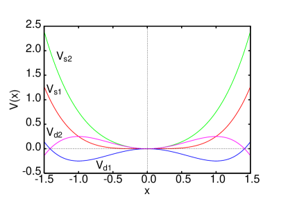
Figure 1: Different possible potentials of a single degree freedom system $V(x)=V_{s1}(x)$, $V_{s2}(x)$, $V_{d1}(x)$ and $V_{d2}(x)$ as defined in Eq. 2 for $\gamma=1.0$ and $\delta=1.0$.

We start our analysis with one of the best known examples exhibiting chaotic solution, namely, the Ueda single well system

$$\frac{{\rm d}^{2}x}{{\rm d}t^{2}}+\alpha\frac{{\rm d}x}{{\rm d}t}+\gamma x^{3}=\mu\sin{\Omega t},$$ (1)

where $x$ is displacement $\alpha\dot{x}$ is linear damping, $\mu\sin{\Omega t}$ is an external excitation while $-\gamma x^{3}$ is a cubic restore force ($\gamma>0$).

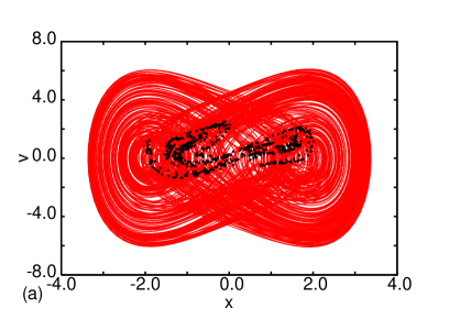
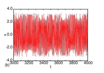
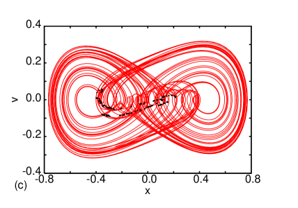
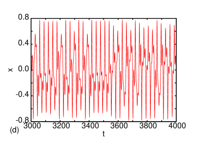
Figure 2: Phase portraits (Fig. 2a,c - with lines) and Poincare maps (Fig. 2a,c - with points) and corresponding time histories $x(t)$ (Fig. 2b,d) for two sets of system (Eq. 1) parameters: Fig. 2a,b with $\gamma=1.0$, $\mu=7.5$, $\alpha=0.05$, $\Omega=1.0$, Fig. 2c,d with $\gamma=1$ $\mu=0.1$, $\alpha=0.05$, $\Omega=0.21$. Top Lyapunov exponents for cases Fig. 2a,b and Fig. 2c,d are $\lambda_{1}=0.111$ and $\lambda_{1}=0.021$, respectively. The initial conditions used in both cases $x(t=0)=0.0$, $v(t=0)=2.5$.

The above example is known from the pioneering Ueda work on chaotic systems [11]. Note that there are substantial differences between a single Ueda well potential $V_{s1}$ without a linear term and a double well Duffing potential $V_{d1}$ or an upside-down reflected double well potential $V_{d2}=-V_{d1}$. On the other hand $V_{s1}$ resembles Duffing potential with hard stiffness $V_{s2}$

$$V_{s1}(x) = \gamma\frac{x^{4}}{4},~{}~{}~{}~{}V_{d1}(x)=\gamma\frac{x^{4}}{4}-\delta\frac{x^{2}}{2},$$ (2)

$$V_{d2}(x) = -\gamma\frac{x^{4}}{4}+\delta\frac{x^{2}}{2},~{}~{}~{}~{}V_{s2}(x)=\gamma\frac{x^{4}}{4}+\delta\frac{x^{2}}{2},$$

where $\gamma$ and $\delta$ are defined positive. In case of $V_{d1}(x)$ and $V_{d2}(x)$ potentials have well defined inflexion points and extrema which correspond to unstable saddle fixed points (Fig. 1) while potentials $V_{s1}(x)$ and $V_{s2}(x)$ are fundamentally different with a single minimum at $x=0$ and without any inflexion points. Note that previous applications of Melnikov theory based on existence of multiple extrema of type $V_{d1}(x)$ or $V_{d2}(x)$.

On the other hand, Chakraborty, in his recent paper [12], noticed that one can expect to apply the Melnikov theory even for a single well potential $V_{s2}$ (Eq. 2) after defining a new coordinate system. Motivated by this conjecture we are going to construct the Melnikov function and derive a necessary condition to system transition into a chaotic motion region.

To explore this possibility further we have performed numerical simulations to find the regions of chaotic solutions (Eq. 1). In Fig. 2 we show the phase portraits and Poincare maps as well as time histories of chaotic solutions. Note Figs. 2a-b correspond to the original Ueda system [11], where $\gamma=1.0$, $\mu=7.5$, $\alpha=0.05$, $\Omega=1.0$. Unfortunately, the large value $\mu$ makes any perturbation method non-relevant while Note Figs. 2c-d, show the chaotic solution for other choice of system parameters: $\gamma=1.0$, $\mu=0.1$, $\alpha=0.05$, $\Omega=0.21$. These chaotic solutions are characterized not only by the fractal strange attractors and non-periodic time series (Figs. 2a-d) but also by positive top Lyapunov exponents $\lambda_{1}=0.111$ and $\lambda_{1}=0.021$ (for $\mu=7.5$ and $\mu=0.1$ respectively). In this second case (2c-d) a perturbation expansion in terms of $\mu$ could be performed. In spite of different system parameters the attractors (given by Poincare maps Figs. 2a and 2c) look similar. To show the regions of chaotic solutions we have plotted the top Lyapunov exponent as a function of $\Omega$ in Fig. 3. For larger $\mu$ we observe the relatively wide region of chaotic solutions (where the top Lyaounov exponent $\lambda_{1}$ has positive values). For smaller $\mu$ chaotic solutions are grouped in the region of low values of an excitation frequency $\Omega$ ($\Omega<0.27$). Interestingly, the Lyapunov exponent, in that region $\lambda_{1}\in[-0.03:0.03]$, is of the same ranges thus the change of $\mu$ does not scale them. Note this is a different region from that discussed by Chakraborty [12] who concentrated on the region where the resonance curve possessed multiple solutions. However in our particular system the chaotic solutions are evidently suppressed by higher excitation frequencies (Figs 3a-b). Thus continuing our research on chaotic solutions appearance in the Ueda system (Eq. 1) (Figs. 2c-d and 3b) we will focus on low frequency region in this paper.

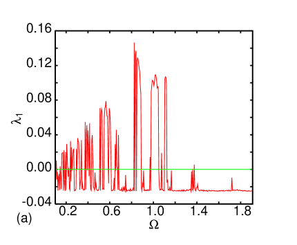
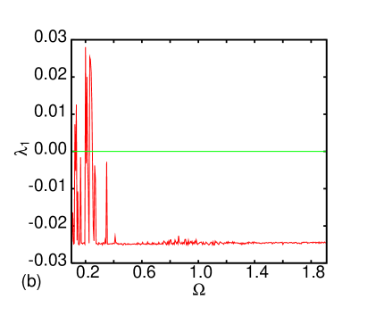
Figure 3: Top Lyapunov exponents versus $\Omega\in[0.1:1.9]$ for two sets of system parameters; $\gamma=1.0$, $\mu=7.5$, $\alpha=0.05$ (Fig 3a) and Fig. with $\gamma=1.0$ $\mu=0.1$, $\alpha=0.05$ (Fig. 3b). For the smallest $\Omega$ the initial condition we assumed to be $x(t=0)=0.0$, $v(t=0)=2.5$ while for any next larger $\Omega$ the final state values of $x$ and $v$ have been used as the initial conditions.

Firstly we will look for homoclinic orbits which can be treated analytically by perturbation methods, namely by the Melnikov method. Such a treatment has been applied to selected problems in science and engineering [2, 3].

2 Approximate solution around the main resonance

In the vicinity of main resonance we assume periodic synchronized solution

$$x=A(t)\sin(\Omega t)+B(t)\cos(\Omega t).$$ (3)

introducing it to Eq. 1 and making use of the following trigonometric identities:

$$(\cos\psi)^{3} = \frac{1}{4}\cos(3\psi)+\frac{3}{4}\cos\psi,$$

$$(\sin\psi)^{3} = -\frac{1}{4}\sin(3\psi)+\frac{3}{4}\sin\psi,$$ (4)

$$\sin(\psi)(\cos\psi)^{2} = \sin(\psi)-\sin(\psi)^{3}=\frac{1}{4}\sin(3\psi)+\frac{1}{4}\sin\psi,$$

$$\cos(\psi)(\sin\psi)^{2} = \cos(\psi)-\cos(\psi)^{3}=-\frac{1}{4}\cos(3\psi)+\frac{1}{4}\cos\psi$$

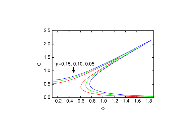
Figure 4: Analytical amplitude $C$, calculated by harmonic balance approximation (Eq. 7), versus $\Omega\in[0.1:1.9]$ in the lowest order for system parameters: $\gamma=1.0$ $\alpha=0.05$, and three values of $\mu$ ($\mu=0.05$, 0.10 and 0.15).

we get

$$\left[\frac{{\rm d}^{2}A}{{\rm d}t^{2}}-\Omega^{2}A+\frac{{\rm d}A}{{\rm d}t}\alpha-\alpha\Omega B+\gamma\frac{3}{4}(A^{3}+AB^{2})-\mu\right]\sin(\Omega t)$$

$$=\gamma(\frac{1}{4}A^{3}-\frac{3}{4}AB^{2})\sin(3(\Omega t))$$ (5)

$$\left[\frac{{\rm d}^{2}B}{{\rm d}t^{2}}-\Omega^{2}B+\frac{{\rm d}B}{{\rm d}t}\alpha+\alpha\Omega A+\gamma\frac{3}{4}(B^{3}+BA^{2})\right]\cos(\Omega t)$$

$$=\gamma(-\frac{1}{4}B^{3}+\frac{3}{4}BA^{2})\cos(3(\Omega t)).$$

In the spirit of the harmonic balance approximation [10] we find fixed points neglecting higher harmonics $\sin(3\Omega t)$ and $\cos(3\Omega t)$ in the lowest approximation. Thus for $\dot{A}=0$ and $\dot{B}=0$

$$-\Omega^{2}A-\alpha\Omega B+\frac{3}{4}\gamma\left(A^{3}+AB^{2}\right)=\mu,$$ (6)

$$-\Omega^{2}B+\alpha\Omega A+\frac{3}{4}\gamma\left(B^{3}+BA^{2}\right)=0.$$

after some simple algebra we get simple equation

$$C^{2}\alpha^{2}\Omega^{2}+C^{2}\left(-\Omega^{2}+\frac{3}{4}\gamma C^{2}\right)^{2}-\mu^{2}=0,$$ (7)

where

$$C^{2}=A^{2}+B^{2}.$$ (8)

The result of an analytical solution (Eq. 7) for the amplitude $C$ versus frequency $\Omega$ has been shown in Fig. 4. One can see the characteristic incline in the resonance in the right hand side. Above $\Omega=0.6$ there are triple solutions where the upper ad bottom ones are stable and the middle one is unstable.

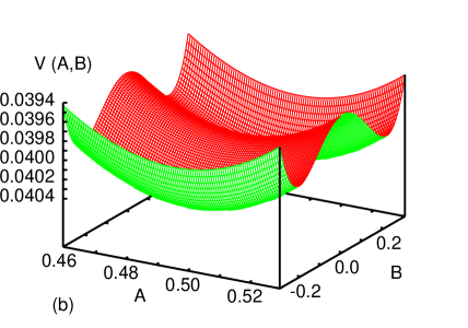
Figure 5: Effective potential $V_{eff}=V_{eff}(A,B)$ for the following system parameters: $\gamma=1.0$ $\mu=0.1$, $\alpha=0.05$ and $\Omega=0.21$ plotted in two different scales (a) and (b) respectively.

3 Melnikov approach beyond harmonic balance

Motivated by Chakraborty [12] we now going beyond the harmonic balance approximation keeping all terms of (Eq. 2) Note, that the higher harmonic terms with $3\Omega t$ can be easily transformed into $2\Omega t$ and $\Omega t$ respectively

$$\cos(3\Omega t) = \left(2\cos(2\Omega t)-1\right)\cos(\Omega t),$$ (9)

$$\sin(3\Omega t) = \left(2\cos(2\Omega t)+1\right)\sin(\Omega t).$$

Thus introducing Eqs. 9 into Eq. 2 and simplifying by $\sin(\Omega t)$ and $\cos(\Omega t)$ we get

$$\frac{{\rm d}^{2}A}{{\rm d}t^{2}} - \Omega^{2}A+\frac{{\rm d}A}{{\rm d}t}\alpha-\alpha\Omega B+\gamma A^{3}-\mu=\gamma\left(\frac{1}{2}A^{3}-\frac{3}{2}AB^{2}\right)\cos(2\Omega t),$$

$$\frac{{\rm d}^{2}B}{{\rm d}t^{2}} - \Omega^{2}B+\frac{{\rm d}B}{{\rm d}t}\alpha+\alpha\Omega A+\gamma B^{3}=\gamma\left(-\frac{1}{2}B^{3}-\frac{3}{2}BA^{2}\right)\cos(2\Omega t).$$ (10)

In this way we have obtained new equations of motion for new coordinates $A(t)$ and $B(t)$ with a parametric excitations.

Defining velocities $v_{A}(t)$ and $v_{B}(t)$ and introducing small parameters into the equation $\epsilon$ and corresponding parameters $\tilde{\gamma}$ and $\tilde{\alpha}$ ($\epsilon\tilde{\gamma}=\gamma$, $\epsilon\tilde{\alpha}=\alpha$) the first order equations of motion as

$$\frac{{\rm d}v_{A}}{{\rm d}t} = \Omega^{2}A-\gamma A^{3}+\epsilon\left(-\tilde{\alpha}v_{A}+\tilde{\alpha}B+\tilde{\gamma}\left(\frac{1}{2}A^{3}-\frac{3}{2}AB^{2}\right)\cos(2\Omega t)\right),$$

$$\frac{{\rm d}A}{{\rm d}t} = v_{A}$$ (11)

$$\frac{{\rm d}v_{B}}{{\rm d}t} = \Omega^{2}B-\gamma A^{3}+\epsilon\left(-\tilde{\alpha}v_{B}-\tilde{\alpha}A+\tilde{\gamma}\left(-\frac{1}{2}B^{3}-\frac{3}{2}A^{2}B\right)\cos(2\Omega t)\right),$$

$$\frac{{\rm d}B}{{\rm d}t} = v_{B}.$$ (12)

The effective unperturbed Hamiltonian for the above set of equations (Eq. 12) can be written

$$H_{eff}=\frac{v_{A}^{2}}{2}+\frac{v_{B}^{2}}{2}+V_{eff}(A,B),$$ (13)

where

$$V_{eff}(A)=\frac{-\Omega^{2}A^{2}}{2}+\frac{\gamma A^{4}}{4}-\mu A+\frac{-\Omega^{2}B^{2}}{2}+\frac{\gamma B^{4}}{4},$$ (14)

and $v_{A}$, $v_{B}$ are effective velocities which define kinetic terms of the Hamiltonian Eq. 13.

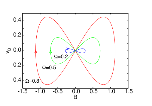
Figure 6: Homoclinic orbits in ($B$, $V_{B}$) plane for $\Omega=0.8$, 0.5, 0.2, respectively

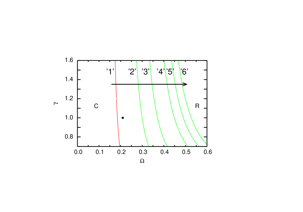
Figure 7: Set of Melnikov curves plotted in a plane of system ($\omega$, $\gamma$). ’1’–’6’ corresponds to $\mu=0.01$, 0.03, 0.05, 0.08, 0.10 and 0.12, respectively. C and R symbolize regions defined by the critical Melnikov curve of possible chaotic and regular solutions.

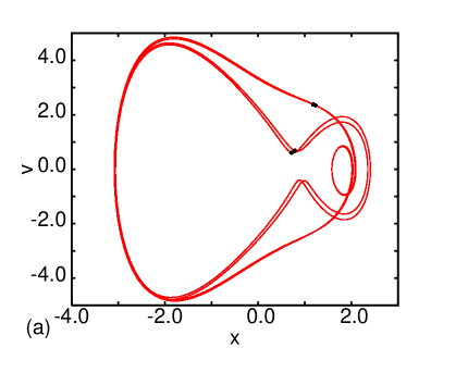
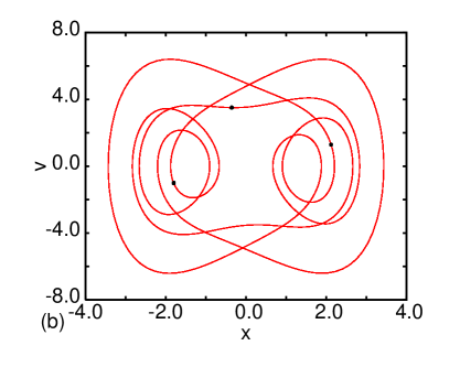
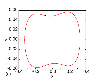
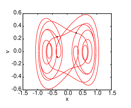
Figure 8: Phase portraits and Poincare maps for system parameters chosen as follows: $\Omega=1.1$, $\mu=7.0$ (Fig. 8a) and $\mu=7.5$ (Fig. 8b); $\Omega=0.21$, $\mu=0.01$ (Fig. 8c) and $\mu=0.35$ (Fig. 8d). The initial condition used in both cases $x(t=0)=0.0$, $v(t=0)=2.5$. The top Lyapunov exponent $\lambda_{1}=0.000$, -0.025, -0.024, -0.024 for Figs 8a-d respectively.

This potential for the chosen system parameters, $\gamma=1.0$ $\mu=0.1$, $\alpha=0.05$ and $\Omega=0.21$, has been plotted in Figs. 5a and b. Note that for more precise mesh (Fig. 5b) we observe double-well structure of potential with degenerated minima energy and a saddle point between them.

Existence of this point with a horizontal tangent makes homoclinic bifurcations of the system possible i.e. transition from a regular to chaotic solution.

Note the characteristic saddle point $[A,B]=[A_{0},0)$ is going to be reached in exactly defined albeit infinite time $t$ corresponding to $+\infty$ and $-\infty$ for stable and unstable orbits, respectively. On the other hand $A_{0}$ can be obtained as the equilibrium fixed point from Eq. 11 and $\epsilon=0$

$$A^{3}-\frac{\Omega^{2}}{\gamma}A-\frac{\mu}{\gamma}=0.$$ (15)

Using the Cardano formula

$$Q=-\frac{\Omega^{6}}{27\gamma^{3}}+\frac{\mu^{2}}{4\gamma^{2}},~{}~{}~{}~{}~{}~{}A_{0}=\sqrt[3]{-\frac{\mu}{\gamma}+\sqrt{Q}}+\sqrt[3]{-\frac{\mu}{\gamma}-\sqrt{Q}}$$ (16)

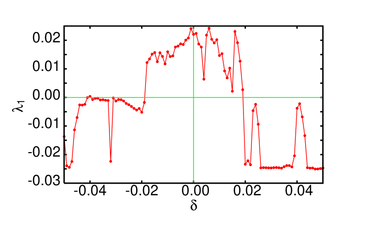
Figure 9: Top Lyapunov exponent against quadratic potential term $\delta$ as in $V_{s2}$ (Eq. 2). For the smallest (negative) $\delta$ the initial conditions we assumed to be $x(t=0)=0.0$, $v(t=0)=2.5$ while for any next larger $\delta$ the final state values of $x$ and $v$ have been used as the initial conditions.

The homoclinic orbit can be derived by assuming that

$$A=A_{0}~{}~{}~{}{\rm and}~{}~{}~{}\lim_{t\rightarrow\pm\infty}B(t)=0.$$ (17)

In this case potential part for $B$ variable reads

$$V_{B}^{\prime}=-\frac{\Omega^{2}}{2}B^{2}+\frac{\gamma}{4}B^{4}.$$ (18)

Assuming the condition $A=A_{0}$ and noting that $V_{B}=0$ at the saddle point ($B=0$) we perform standard analysis on energy conservation formula

$$0=\frac{v_{B}^{2}}{2}+V_{B}^{\prime}(B)$$ (19)

and after integration we get

$$-\frac{1}{\Omega}\ln{\left(\frac{\sqrt{\frac{2\Omega^{2}}{\gamma}}+\sqrt{\frac{2\Omega^{2}}{\gamma}-B^{2}}}{B}\right)}=t+t_{0},$$ (20)

where $t_{0}$ is a time like integration constant.

Finally the homoclinic orbit is given by time dependent coordinate $B(t)=B^{*}(t)$

$$B^{*}(t)=\sqrt{\frac{2}{\gamma}}\frac{\Omega}{\cosh{(\Omega(t+t_{0}))}}$$ (21)

and a corresponding velocity $v_{B}(t)=v_{B}^{*}(t)$

$$v_{B}^{*}(t)=-\sqrt{\frac{2}{\gamma}}\frac{\Omega^{2}\sinh{(\Omega(t+t_{0}))}}{\cosh^{2}{(\Omega(t+t_{0}))}}.$$ (22)

The homoclinic orbits for the same system parameters $\gamma$ and $\mu$ as in Fig. 5 and assumed three values of excitation frequency ($\Omega=0.8$, 0.5, 0.2) has been plotted in Fig. 6. Interestingly, for higher $\Omega$ we observe the effect of blowing the length of homoclinic loops and corresponding areas inside.

In case of perturbed orbits $W^{S}$ and $W^{U}$ the distance between them is given by the Melnikov function $M(t_{0})$:

$$M(t_{0})=\int_{-\infty}^{+\infty}h(B^{*},v_{B}^{*})\wedge g(B^{*},v_{B}^{*}){\rm d}t$$ (23)

where the corresponding differential forms $h$ as the gradient of unperturbed Hamiltonian (Eq. 13) (for $A(t)=A_{0}$) leading to equations of motion

$$\frac{\partial H^{0}}{\partial B}=-\dot{v_{B}},~{}~{}~{}\frac{\partial H^{0}}{\partial v_{B}}=\dot{B},$$ (24)

while $g$ as its perturbation form of the above

$$h = \left(\Omega^{2}B+\gamma B^{3}\right){\rm d}B+v_{B}{\rm d}v_{B},$$ (25)

$$g = \left(-\tilde{\alpha}v_{B}-\tilde{\alpha}\Omega A_{0}+\tilde{\gamma}\left(-\frac{1}{2}B^{3}-\frac{3}{2}BA^{2}\right)\cos(2\Omega t)\right){\rm d}x$$

are defined on homoclinic manifold $(B,v_{B})=(B^{*},v_{B}^{*})$. Finally the Melnikov integral is given by

$$M(t_{0}) = \int_{-\infty}^{+\infty}{\rm d}t~{}~{}\left(-\tilde{\alpha}v_{B}^{*}-\tilde{\alpha}\Omega A_{0}+\tilde{\gamma}\left(-\frac{1}{2}B^{*3}-\frac{3}{2}B^{*}A^{*2}\right)\cos(2\Omega t)\right)v_{B}^{*}$$

(26)

After substituting $B^{*}(t)$ and $v_{B}^{*}(t)$ by formulae given in Eq. 6 and $A^{*}(t)=A_{0}$ (Eq. 16) we get (see Appendix A)

$$M(t_{0}) = -\frac{4}{3}\tilde{\alpha}\frac{\Omega^{3}}{\gamma}+\frac{16}{3}\tilde{\gamma}\frac{\Omega^{4}}{\gamma\sqrt{\gamma}}\pi{\rm e}^{-\pi}\sin(2\Omega t_{0})$$ (27)

$$+ 12\tilde{\gamma}A_{0}^{2}\frac{\Omega^{2}}{\gamma}\pi{\rm e}^{-\pi}\sin(2\Omega t_{0}).$$

In the Melnikov theory $M\sim d$ [1, 2, 3], where $d$ is the distance between stable and unstable manifolds. Simple zero of the Melnikov function $M$ is associated with the cross-section of these manifolds indicating global homoclinic bifurcation. In our case this condition (for the set of parameters: $\alpha$, $\gamma$, $\Omega$ and $A_{0}$ which a function of $\mu$, $\gamma$ and $\Omega$ $A_{0}(\mu,\gamma,\Omega)$ (see Eqs.15-16) is fulfilled for $|\sin(2\Omega t_{0})|=0$

$$\alpha\Omega=(12\Omega^{2}\sqrt{\gamma}+9A_{0}^{2}\sqrt{\gamma})\pi{\rm e}^{-\pi}.$$ (28)

The analytical results for critical parameters $\gamma=\gamma_{c}$ and $\Omega=\Omega_{c}$ basing on this equation are shown in Fig. 7 for $\mu=0.01$, 0.03, 0.05, 0.08, 0.10 and 0.12. respectively. Left and right handed regions denoted for each curve as C and R respectively are related to possible ”Chaotic” and ”Regular” solutions. The results show that for larger $\gamma$ chaotic solution is more limited. This tendency is better visible for a larger excitation amplitude $\mu$. Note the formerly investigated chaotic solution has been indicated by a singular point in the figure. Account for that case $\mu$ was chosen as 0.1 one can easily see that this solution match with the analytical prediction. We have also checked that our system undergoes typical period doubling cascade showing also three points solution as well (defined on Poincare maps) Figs. 8b,d. In case of ) This regulars solution often accompany a chaotic solution. Note also that for one of presented solutions (in Fig. 8a) the Lyapunov exponent was approximately 0 indicating a doubling period bifurcation point. A typical solution, synchronized with an excitation term, has been shown in Fig. 8c.

4 Summary and Conclusions

In summary we have performed the Mielnikov analysis for the Ueda system with a single well potential. Through transforming the system to new variables it was possible to investigate the Mielnikov criterion for a global homoclinic bifurcation from regular to chaotic oscillations.

Our investigation was limited purposely to a small frequency $\Omega$ where the chaotic solutions emerge numerically (Figs. 2c,d). However for different nonliner systems involving nonlinear damping terms and the self-excitation effects [13] the region of chaotic solutions could be different. The main simplification in our treatment was the assumption $A(t)=A_{0}=$const. In a more general case one should expect additional time dependence of the amplitude $A$ which could create an additional shift of the critical lines in Fig. 7. This shift should be dependent on $\Omega$, which influences strongly the size of homoclinic orbits Fig. 6. Consequently, for our system, in the limit of large $\Omega$ the size of the homoclinc orbit is so large that condition $A(t)=$const. cannot be applied.

Our results for the top Lyapunov exponent (Fig. 9) show also that the chaotic solution was preserved in presence of a small linear force term $\delta$ (see $V_{s2}$ in Eq. 2) so the method presented here can be generalized to the Duffing system having linear and cubic force terms.

References

[1] V.K. Melnikov, On the stability of the center for time periodic
perturbations,
Trans. Moscow Math. Soc. 12 (1963) 1–57.
[2] J. Guckenheimer, P. Holms, Nonlinear
Oscillations,
Dynamical Systems and Bifurcations of Vectorfields, Springer, New York
1983.
[3] S. Wiggins, Introduction to Applied Nonlinear
Dynamical
Systems and Chaos, Spinger, New York 1990.
[4] E. Tyrkiel,
On the role of chaotic saddles in generating chaotic dynamics in nonlinear
driven oscillators, Int. J. Bifurcation and Chaos 15 (2005) 1215–1238.
[5] W. Szemplińska-Stupnicka, The analytical
predictive criteria for chaos and escape in nonlinear oscillators: A
survey, Nonlinear Dynamics
7 (1995) 129-147.
[6]
G. Litak, M. Borowiec, Oscillators with asymmetric single and double well
potentials: Transition to chaos revisited, Acta Mechanica 184 (2006) 47- 59.
[7]
G. Litak, A. Syta, M. Borowiec, Suppression of chaos by weak
resonant excitations in a nonlinear oscillator with a non-symmetric
potential, Chaos, Solitons & Fractals
32 (2007) 694–701.
[8] W. Szemplińska-Stupnicka, J. Rudowski,
Bifurcations phenomena in a nonlinear oscillator: Approximate analytical
studies versus computer simulation results, Physica D 66 (1993)
368–380.
[9] T. Kapitaniak, Analytical method of controling
chaos in Duffing
oscillator, Journal of
Sound and Vibration 163 (1993) 182–187.
[10] T. Kapitaniak, Chaotic Oscillations in
Mechanical Systems,
Manchester University Press, Manchester 1991.
[11] Y. Ueda, Randomly transitional phenomena in the system
governed
by Duffing’s equation, Journal of Statistical Physics 20 (1979)
181–196.
[12] G. Chakraborty, A conjecture on route to chaos
in a hard Duffing
oscillator by homoclinic entanglement, J. Sound Vibr. 294 (2006) 235–440.
[13]
G. Litak, G. Spuz-Szpos, K. Szabelski, J. Warmiński, Vibration analysis
of self-excited system with parametric forcing and nonlinear stiffness,
Int. J. Bifurcation and Chaos 9 (1999) 493–504.