nlin.SI/0610017
AEI-2006-074
PUTP-2211

1 Introduction and Overview

Gauge/string dualities give promise to explain stringy aspects of quantum chromodynamics and to deepen our understanding of quantum gravity. They relate two seemingly different quantum field theory models: gauge theories in various spacetime dimensions and string theories based on a two-dimensional world sheet QFT. The most elaborate such duality is Maldacena’s AdS/CFT correspondence [1, 2, 3]. It identifies a string theory on an $AdS_{d+1}\times X$ background with a conformal field theory on the $d$-dimensional boundary of the $AdS_{d+1}$ space. The key example of AdS/CFT is the conjectured exact duality between IIB superstrings on $AdS_{5}\times S^{5}$ and $\mathcal{N}=4$ extended supersymmetric gauge theory in four spacetime dimensions. We shall focus on this particular duality in the present work.

AdS/CFT-dual models typically have at least two parameters: a coupling constant $\lambda$ and a genus-counting parameter $g_{\mathrm{s}}$. While the genus-counting parameter is natural within string theory, it is given by $4\pi g_{\mathrm{s}}/\lambda=1/N_{\mathrm{c}}$ in a $\mathrm{U}(N_{\mathrm{c}})$ gauge theory. The equivalence of the latter two parameters was shown a long time ago by ’t Hooft [4]. A suitable coupling constant for gauge theory is the ’t Hooft coupling $\lambda=g_{\mathrm{\scriptscriptstyle YM}}^{2}N_{\mathrm{c}}$ and for string theory it is related to the string tension by $\lambda=1/\alpha^{\prime 2}$. The relationship between these parameters is less obvious because the perturbative regimes of both models do not overlap: String theory is strongly coupled where gauge theory is perturbative and vice versa. The distinctness of perturbative regimes is actually what makes the AdS/CFT possible despite the fact that the perturbative models do not resemble each other remotely. The strong/weak nature of AdS/CFT can thus be viewed ambivalently: On the one hand, it gives access to hitherto inaccessible regimes in both modes. However, these predictions would require us to put all our faith into the correspondence. If we prefer not to, on the other hand, the strong/weak nature prevents almost all tests of the conjectured duality as we cannot compute corresponding quantities in both participating models simultaneously. Nevertheless some tests are possible and confirm the duality, cf. the reviews [5, 6]. Most of these tests involve quantities which are protected from receiving quantum corrections and which can therefore be carried easily from one perturbative regime to the other.

At least in the planar limit, $N_{\mathrm{c}}=\infty$, some progress towards a comparison of quantities which depend non-trivially on the coupling constant $\lambda$ has been made in recent years. To absorb most factors of $\pi$ and $2$ we shall use a normalised coupling constant

$$g=\frac{\sqrt{\lambda}}{4\pi}\,.$$ (1.1)

The suspected exact integrability of planar $\mathcal{N}=4$ super Yang-Mills (SYM) theory [7, 8, 9], see also [10, 11, 12], and of non-interacting IIB superstring theory on $AdS_{5}\times S^{5}$ [13, 14, 15] provides hope that their spectrum can be computed exactly at finite coupling $g$ by means of Bethe equations [16], cf. the reviews [17, 18, 19] and [20].

The underlying integrable model of AdS/CFT is best described as a two-dimensional sigma model [21] in the limit of perturbative string theory and as a spin chain in the limit of perturbative gauge theory. Many results and techniques have been developed for these two types of integrable models. For instance, a general framework exists for the solution of a large class of integrable spin chains. The Bethe equations for these chains can easily be written down once the symmetry and representation content is given [22]. They are in general founded strongly on the symmetry algebra and representation theory of the model. Unfortunately, the standard form of rational Bethe equations does not apply to the spin chain of $\mathcal{N}=4$ SYM, a fact which is explained by its slightly unusual form: While almost all known integrable spin chain Hamiltonians induce interactions between two neighbouring spin sites, the $\mathcal{N}=4$ SYM spin chain Hamiltonian consists of interactions with a longer range and between more than two sites. Moreover, in standard spin chains the Hamiltonian alias the time translation generator factors from the remaining symmetry group $G$ as $\mathbb{R}\times G$. Here, the Hamiltonian is merely one generator of the irreducible symmetry group $\mathrm{PSU}(2,2|4)$ of AdS/CFT. This has some important and puzzling implications for the representation theory of the model. Similar problems are encountered for the stringy sigma model of AdS/CFT which is not strictly Poincaré-invariant unlike many of the well-known integrable sigma models. All this means that the standard solution for integrable models does not apply. Nevertheless the Bethe equations for AdS/CFT are somewhat similar to standard rational Bethe equations and they display signs of the underlying $\mathfrak{psu}(2,2|4)$ symmetry. It is therefore conceivable that some unified framework for the treatment of the AdS/CFT and standard spin chains can be found. Such a framework would provide more insight into the foundations of the integrable structures of AdS/CFT, but may also contribute to the general understanding of integrable structures. It is the aim of this paper to take some steps towards such a framework.

The main objects of investigation in this article will be the residual algebra, the S-matrix and transfer matrices. We will assume that the $\mathcal{N}=4$ SYM spin chain has already been transformed to a particle model by means of a coordinate space Bethe ansatz [23, 24, 25], see also [26]. In other words, spin flips about a ferromagnetic vacuum are considered as momentum-carrying particles. For the string sigma model we will assume that a light cone gauge has reduced the spectrum to physical excitation modes also yielding a particle model. In the particle model picture the full $\mathrm{PSU}(2,2|4)$ symmetry of AdS/CFT is spontaneously broken by the vacuum to some residual symmetry. The latter consists of two copies of the supergroup $\mathrm{PSU}(2|2)$ with central extensions [27, 28]. Section 2 deals with the representation theory of the centrally extended $\mathfrak{psu}(2|2)$ algebra.

Symmetry is a central ingredient for the construction and investigation of the S-matrix performed in the subsequent Sec. 3. The S-matrix [25, 16, 27] describes the asymptotic wave functions of multi-particle states on a vacuum of infinite length. In this section we shall derive and compare different notations to deal with multi-particle states and then derive the S-matrix as well as its properties. Most importantly, we will find a simple proof of the Yang-Baxter equation (YBE) making full use of representation theory. The YBE then enables us to diagonalise the S-matrix by means of a nested Bethe ansatz. Finally we consider multi-particle states on a compact vacuum by imposing periodicity conditions on the wave function. These are the (asymptotic) Bethe equations of the system.

In Sec. 5 we shall proceed towards an analytic Bethe ansatz [29] for a spin chain with centrally extended $\mathfrak{psu}(2|2)$ symmetry. The central objects of the analytic Bethe ansatz are transfer matrices whose eigenvalues we shall obtain by reverse-engineering. In other words, we will assume that the analytic Bethe ansatz leads to the same Bethe equations that were derived before. This step fixes large parts of the structure of the transfer matrix eigenvalues. Considering some explicit states, we can write down the spectrum of transfer matrices in several representations.

Finally, we would like to sketch how to assemble the transfer matrices of two $\mathfrak{psu}(2|2)$ spin chains to a transfer matrix of the AdS/CFT model with $\mathfrak{psu}(2,2|4)$ symmetry. This Sec. 6 is of a very explorative character; it does not provide conclusive answers, but rather starting points and clues for further investigations. A rigorous treatment would require a full investigation of the abelian phase factor of the S-matrix which is beyond the scope of the present paper. This phase should obey a crossing relation derived by Janik [30] leading to a very intricate analytic structure [31, 32]. Hopefully, an analytic Bethe ansatz will be obtained elsewhere by a rigorous treatment of the analytic structure of the transfer matrix eigenvalue.

In the interlude of Sec. 4 we investigate the connection between the AdS/CFT correspondence and the one-dimensional Hubbard model [33]. The latter is an exceptional spin chain model because it lies within the standard class of nearest-neighbour models described above, but its Bethe equations, the so-called Lieb-Wu equations [34], take a non-standard trigonometric form. Its integrable structures are known to a large extent, cf. [35] for a review, but they also take an unusual form. For example, Shastry’s R-matrix for the Hubbard chain [36] is not of a difference form; it is rather a function which genuinely depends on two independent spectral parameters. It is fair to say that the foundations of this integrable system are not yet fully understood. In particular the relation to representation theory, which is a central aspect of standard integrable spin chains, remains obscure. In this paper we will show that the Lieb-Wu equations and Shastry’s R-matrix appear within AdS/CFT as parts of the Bethe equations and the S-matrix. Both models are therefore based on the same integrable structures. This provides a novel way of looking at the Hubbard chain, in particular at the underlying symmetry and representation theory. It should be noted that this connection between the two models is complementary to the one discovered earlier in [37]: There are some similarities between the two observations, but they neither explain nor exclude each other.

2 Centrally Extended $\mathfrak{su}(2|2)$

In this section we introduce the algebra on which the spin chain model is based. We shall denote it by $\mathfrak{h}$.

2.1 The Algebra

The centrally extended $\mathfrak{su}(2|2)$ algebra $\mathfrak{h}=\mathfrak{psu}(2|2)\ltimes\mathbb{R}^{3}$, see e.g. [38], consists of the $\mathfrak{su}(2)\times\mathfrak{su}(2)$ rotation generators $\mathfrak{R}^{a}{}_{b}$, $\mathfrak{L}^{\alpha}{}_{\beta}$, the supersymmetry generators $\mathfrak{Q}^{\alpha}{}_{b}$, $\mathfrak{S}^{a}{}_{\beta}$ and the central charges $\mathfrak{C},\mathfrak{P},\mathfrak{K}$. The non-trivial commutators are

$$[\mathfrak{R}^{a}{}_{b},\mathfrak{J}^{c}]\mathrel{} = \mathrel{}\delta^{c}_{b}\mathfrak{J}^{a}-{\textstyle\frac{1}{2}}\delta^{a}_{b}\mathfrak{J}^{c},$$

$$[\mathfrak{L}^{\alpha}{}_{\beta},\mathfrak{J}^{\gamma}]\mathrel{} = \mathrel{}\delta^{\gamma}_{\beta}\mathfrak{J}^{\alpha}-{\textstyle\frac{1}{2}}\delta^{\alpha}_{\beta}\mathfrak{J}^{\gamma},$$

$$\{\mathfrak{Q}^{\alpha}{}_{a},\mathfrak{S}^{b}{}_{\beta}\}\mathrel{} = \mathrel{}\delta^{b}_{a}\mathfrak{L}^{\alpha}{}_{\beta}+\delta^{\alpha}_{\beta}\mathfrak{R}^{b}{}_{a}+\delta^{b}_{a}\delta^{\alpha}_{\beta}\mathfrak{C},$$

$$\{\mathfrak{Q}^{\alpha}{}_{a},\mathfrak{Q}^{\beta}{}_{b}\}\mathrel{} = \mathrel{}\varepsilon^{\alpha\beta}\varepsilon_{ab}\mathfrak{P},$$

$$\{\mathfrak{S}^{a}{}_{\alpha},\mathfrak{S}^{b}{}_{\beta}\}\mathrel{} = \mathrel{}\varepsilon^{ab}\varepsilon_{\alpha\beta}\mathfrak{K}.$$ (2.1)

The symbols $\mathfrak{J}^{a},\mathfrak{J}^{\alpha}$ represent any generator with an upper index.

2.2 Outer Automorphism

The algebra $\mathfrak{h}$ has an $\mathfrak{sl}(2)$ outer automorphism. This can be seen most easily when we rearrange the generators into multiplets of the automorphism:

$$\mathfrak{C}^{\mathfrak{a}}{}_{\mathfrak{b}}=\left(\begin{array}[]{ll}-\mathfrak{C}&+\mathfrak{P}\\ -\mathfrak{K}&+\mathfrak{C}\end{array}\right),\qquad\mathfrak{J}^{a\beta\mathfrak{c}}=\left(\begin{array}[]{c}\varepsilon^{ad}\mathfrak{Q}^{\beta}{}_{d}\\ \varepsilon^{\beta\delta}\mathfrak{S}^{a}{}_{\delta}\end{array}\right).$$ (2.2)

The non-trivial commutators of $\mathfrak{h}$ are now written in a manifestly $\mathfrak{sl}(2)$-invariant way

$$[\mathfrak{R}^{a}{}_{b},\mathfrak{R}^{c}{}_{d}]\mathrel{} = \mathrel{}\delta_{b}^{c}\mathfrak{R}^{a}{}_{d}-\delta^{a}_{d}\mathfrak{R}^{c}{}_{b},$$

$$[\mathfrak{L}^{\alpha}{}_{\beta},\mathfrak{L}^{\gamma}{}_{\delta}]\mathrel{} = \mathrel{}\delta_{\beta}^{\gamma}\mathfrak{L}^{\alpha}{}_{\delta}-\delta^{\alpha}_{\delta}\mathfrak{L}^{\gamma}{}_{\beta},$$

$$[\mathfrak{R}^{a}{}_{b},\mathfrak{J}^{c\delta\mathfrak{e}}]\mathrel{} = \mathrel{}\delta_{b}^{c}\mathfrak{J}^{a\delta\mathfrak{e}}-{\textstyle\frac{1}{2}}\delta_{b}^{a}\mathfrak{J}^{c\delta\mathfrak{e}},$$

$$[\mathfrak{L}^{\alpha}{}_{\beta},\mathfrak{J}^{c\delta\mathfrak{e}}]\mathrel{} = \mathrel{}\delta_{\beta}^{\delta}\mathfrak{J}^{c\alpha\mathfrak{e}}-{\textstyle\frac{1}{2}}\delta_{\beta}^{\alpha}\mathfrak{J}^{c\delta\mathfrak{e}},$$

$$\{\mathfrak{J}^{a\beta\mathfrak{c}},\mathfrak{J}^{d\epsilon\mathfrak{f}}\}\mathrel{} = \mathrel{}\varepsilon^{ad}\varepsilon^{\epsilon\kappa}\varepsilon^{\mathfrak{cf}}\mathfrak{L}^{\beta}{}_{\kappa}+\varepsilon^{ak}\varepsilon^{\epsilon\beta}\varepsilon^{\mathfrak{cf}}\mathfrak{R}^{d}{}_{k}+\varepsilon^{ad}\varepsilon^{\epsilon\beta}\varepsilon^{\mathfrak{fk}}\mathfrak{C}^{\mathfrak{c}}{}_{\mathfrak{k}}.$$ (2.3)

We can introduce the $\mathfrak{sl}(2)$ generators $\mathfrak{B}^{\mathfrak{a}}{}_{\mathfrak{b}}$, and their non-trivial commutators are consequently

$$[\mathfrak{B}^{\mathfrak{a}}{}_{\mathfrak{b}},\mathfrak{B}^{\mathfrak{c}}{}_{\mathfrak{d}}]\mathrel{} = \mathrel{}\delta_{\mathfrak{b}}^{\mathfrak{c}}\mathfrak{B}^{\mathfrak{a}}{}_{\mathfrak{d}}-\delta^{\mathfrak{a}}_{\mathfrak{d}}\mathfrak{B}^{\mathfrak{c}}{}_{\mathfrak{b}},$$

$$[\mathfrak{B}^{\mathfrak{a}}{}_{\mathfrak{b}},\mathfrak{J}^{c\delta\mathfrak{e}}]\mathrel{} = \mathrel{}\delta_{\mathfrak{b}}^{\mathfrak{e}}\mathfrak{J}^{c\delta\mathfrak{a}}-{\textstyle\frac{1}{2}}\delta_{\mathfrak{b}}^{\mathfrak{a}}\mathfrak{J}^{c\delta\mathfrak{e}},$$

$$[\mathfrak{B}^{\mathfrak{a}}{}_{\mathfrak{b}},\mathfrak{C}^{\mathfrak{c}}{}_{\mathfrak{d}}]\mathrel{} = \mathrel{}\delta_{\mathfrak{b}}^{\mathfrak{c}}\mathfrak{C}^{\mathfrak{a}}{}_{\mathfrak{d}}-\delta^{\mathfrak{a}}_{\mathfrak{d}}\mathfrak{C}^{\mathfrak{c}}{}_{\mathfrak{b}}.$$ (2.4)

The enlarged algebra shall be called $\mathfrak{h}_{\mathrm{out}}=\mathfrak{sl}(2)\ltimes\mathfrak{h}$. Note that we will mostly not consider the enlarged algebra $\mathfrak{h}_{\mathrm{out}}$ because its representations are substantially different from those of $\mathfrak{h}$ which are of interest to us. Nevertheless, we might keep the Cartan generator of $\mathfrak{sl}(2)$; let us denote it by $\mathfrak{B}$ and the extended algebra by $\mathfrak{h}_{+}=\mathbb{R}\ltimes\mathfrak{h}$. This generator is the same as the abelian automorphism of the algebra $\mathfrak{pu}(2|2)=\mathbb{R}\times\mathfrak{psu}(2|2)$. One can embed it into the $\mathfrak{sl}(2)$ matrix as

$$\mathfrak{B}^{\mathfrak{a}}{}_{\mathfrak{b}}=\left(\begin{array}[]{ll}-\mathfrak{B}&+\mathfrak{B}^{+}\\ -\mathfrak{B}^{-}&+\mathfrak{B}\end{array}\right).$$ (2.5)

The appearance of the automorphism can also be understood in terms of the contraction of the exceptional superalgebra $\mathfrak{d}(2,1;\varepsilon,\mathbb{R})$ with $\varepsilon\to 0$ presented in [27]. When setting $\varepsilon=0$ without rescaling some of the generators, however, the algebra would be $\mathfrak{d}(2,1;0,\mathbb{R})=\mathfrak{sl}(2)\ltimes\mathfrak{psu}(2|2)$. Therefore, the generators $\mathfrak{B}^{\mathfrak{a}}{}_{\mathfrak{b}}$ and $\mathfrak{C}^{\mathfrak{a}}{}_{\mathfrak{b}}$ originate from the same $\mathfrak{sl}(2)$ factor in $\mathfrak{d}(2,1;\varepsilon,\mathbb{R})$ by taking two different limits $\varepsilon\to 0$. Curiously, both triplets of generators can coexist in $\mathfrak{h}_{\mathrm{out}}$.

Note that the bi-linear combination

$$\mathfrak{\vec{C}}^{2}={\textstyle\frac{1}{2}}\mathfrak{C}^{\mathfrak{a}}{}_{\mathfrak{b}}\mathfrak{C}^{\mathfrak{b}}{}_{\mathfrak{a}}=\mathfrak{C}^{2}-\mathfrak{P}\mathfrak{K}$$ (2.6)

is invariant under $\mathfrak{sl}(2)$ and therefore under the complete algebra $\mathfrak{h}_{\mathrm{out}}$.

2.3 Representations

Here we consider representations of $\mathfrak{h}$ for which all the central charges $\mathfrak{C},\mathfrak{P},\mathfrak{K}$ have well-defined numerical eigenvalues $C,P,K$. We furthermore demand that the $\mathfrak{sl}(2)$-invariant combination $C^{2}-PK$, cf. (2.6), is positive.

In order to understand these representations we can make use of the outer automorphism to relate them to representations of $\mathfrak{su}(2|2)$, which have been studied in [39, 40, 41, 42, 43]. Under the automorphism, the charge eigenvalues $(C,P,K)$ transform as a space-like vector of $\mathfrak{so}(2,1)=\mathfrak{sl}(2)$. We can thus transform $(C,P,K)$ to $(\pm\sqrt{C^{2}-PK},0,0)$. The representation becomes a representation of $\mathfrak{su}(2|2)$ with central charge $\pm\sqrt{C^{2}-PK}$. The representations of $\mathfrak{h}$ with well-defined eigenvalues of the central charges are nothing but representations of $\mathfrak{su}(2|2)$ modulo a $\mathfrak{sl}(2)$-rotation of the algebra.

Let us now discuss two relevant types of finite-dimensional irreducible representations of $\mathfrak{h}$. We shall call them long (typical) and short (atypical).

Figure 1: Young tableaux for long and short representations $\{m,n\}$ and $\langle m,n\rangle$. The label $\ast$ represents a stack of arbitrarily many boxes. A single box represents the fundamental representation $\langle 0,0\rangle$.

Long Multiplets.

A long multiplet of $\mathfrak{h}$ will be denoted by

$$\{m,n;C,P,K\}=\{m,n;\vec{C}\}.$$ (2.7)

Here $\vec{C}=(C,P,K)$ are the eigenvalues of the central charges. The non-negative integers $m,n$ are Dynkin labels specifying multiplets of $\mathfrak{su}(2)\times\mathfrak{su}(2)$. The overall dimension of this multiplet is $16(m+1)(n+1)$ distributed evenly among the gradings.

The corresponding representations of $\mathfrak{su}(2|2)$ are specified by the Dynkin labels ${[m;r;n]}$ with $r=\pm\sqrt{C^{2}-PK}-{\textstyle\frac{1}{2}}n+{\textstyle\frac{1}{2}}m$. Note that the middle Dynkin label $r$ is related to the $\mathfrak{su}(2|2)$ central charge by $C={\textstyle\frac{1}{2}}n-{\textstyle\frac{1}{2}}m+r$. In fact, one class of representations with fixed $m,n,|\vec{C}|$ of $\mathfrak{h}$ generally interpolates between two representations of $\mathfrak{su}(2|2)$ with $C=\pm|C|$ (unless $C=0$). The Young tableaux for long representations are depicted in Fig. 1, see [44] for the use of Young tableaux in superalgebras.

In terms of the bosonic subalgebra $\mathfrak{su}(2)\times\mathfrak{su}(2)$ the multiplet decomposes into the components

$$\left\{\begin{array}[]{cccc}[m+0,n+0]&[m+0,n+0]&[m+0,n+0]&[m+0,n+0]\\ {}[m+2,n+0]&[m+0,n+2]&[m-2,n+0]&[m+0,n-2]\\ \hline\cr[m+1,n+1]&[m+1,n+1]&[m-1,n+1]&[m-1,n+1]\\ {}[m+1,n-1]&[m+1,n-1]&[m-1,n-1]&[m-1,n-1]\end{array}\right\}.$$ (2.8)

Here $[m,n]$ specifies the $\mathfrak{su}(2)\times\mathfrak{su}(2)$ Dynkin labels, i.e. $m,n$ are twice the spins of the multiplets. The bar separates components with different grading.

For small values of $m,n$ special care has to be taken in the decomposition. We should then treat all components of the form $[-1,n]$ or $[m,-1]$ as absent. The components $[-2,n]$ and $[m,-2]$ should be treated as $[0,n]$ and $[m,0]$, respectively, but with multiplicity $-1$ (they will always cancel against some other component).

Short Multiplets.

A short multiplet will be denoted by

$$\langle m,n;C,P,K\rangle=\langle m,n;\vec{C}\rangle\quad\mbox{with}\quad\vec{C}^{2}=C^{2}-PK={\textstyle\frac{1}{4}}(n+m+1)^{2}.$$ (2.9)

Again $m,n$ are non-negative integers representing Dynkin labels of $\mathfrak{su}(2)\times\mathfrak{su}(2)$. The overall dimension of this multiplet is $4(m+1)(n+1)+4mn$ distributed evenly among the gradings.

The Dynkin labels of the corresponding $\mathfrak{su}(2|2)$ representations are $[m-1;m;n]$ (for $m=0$ we should pick $[0;0;n+1]$ instead) or by $[m;-n;n-1]$ (for $n=0$ we should pick $[m+1;0;0]$ instead). These representations are atypical. The Young tableaux for short representations are presented in Fig. 1.

The $\mathfrak{su}(2)\times\mathfrak{su}(2)$ components of a short multiplet are

$$\left\{\begin{array}[]{cccc}[m-1,n+0]&[m-1,n+0]&[m+1,n+0]&[m-1,n-2]\\ \hline\cr[m+0,n-1]&[m+0,n-1]&[m+0,n+1]&[m-2,n-1]\end{array}\right\}.$$ (2.10)

Interesting special cases are the two series of multiplets

$$\langle m,0;\vec{C}\rangle\mathrel{} \to \mathrel{}\left\{\begin{array}[]{cc|c}[m-1,0]&[m+1,0]&[m+0,1]\end{array}\right\},$$ (2.12)

$$\langle 0,m;\vec{C}\rangle\mathrel{} \to \mathrel{}\left\{\begin{array}[]{cc|c}[0,m-1]&[0,m+1]&[1,m+0]\end{array}\right\}.$$ (2.14)

In particular, the single multiplet $\langle 0,0;\vec{C}\rangle$ being part of both series deserves further consideration: It is the smallest non-trivial multiplet, it has two bosonic and two fermionic components

$$\left\{\begin{array}[]{c|c}[1,0]&[0,1]\end{array}\right\}.$$ (2.15)

It can thus be viewed as the fundamental multiplet of $\mathfrak{h}$ in analogy to the one of $\mathfrak{su}(2|2)$. It shall be denoted as

$$\langle C,P,K\rangle:=\langle 0,0;C,P,K\rangle\quad\mbox{or}\quad\langle\vec{C}\rangle:=\langle 0,0;\vec{C}\rangle,$$ (2.16)

and will be discussed in detail in Sec. 2.4. The former multiplets (2.12) can be considered totally (anti)symmetric products of the fundamental multiplet.

Anomalous Multiplets.

There are further types of finite-dimensional multiplets. These include at least the trivial multiplet $\langle\cdot\rangle$ and several types of adjoint multiplets. Both the singlet and the adjoint multiplets have all central charges equal zero, $C=P=K=0$.

The minimal adjoint multiplet $\langle\mathrm{adj}_{\mathfrak{psu}(2|2)}\rangle$ has the components

$$\left\{\begin{array}[]{cc|cc}[2,0]&[0,2]&[1,1]&[1,1]\end{array}\right\},$$ (2.17)

corresponding to the algebra $\mathfrak{psu}(2|2)$. The bigger adjoints may have several of the additional components of the extended algebra $\mathfrak{h}_{\mathrm{out}}$. Note that the components corresponding to central charges may form submultiplets of $\mathfrak{h}$.

Multiplet Splitting.

$\parbox{56.9055pt}{\centering\includegraphics[scale={1}]{n4trans.Fig.Tableaux.Splitting.1.eps}\@add@centering}=\parbox{56.9055pt}{\centering\includegraphics[scale={1}]{n4trans.Fig.Tableaux.Splitting.2.eps}\@add@centering}\oplus\parbox{56.9055pt}{\centering\includegraphics[scale={1}]{n4trans.Fig.Tableaux.Splitting.3.eps}\@add@centering}$

Figure 2: Diagrammatic representation of multiplet splitting (2.18) using Young tableaux. The filled boxes on the right hand side are to be removed leaving short representations.

A long multiplet $\{m,n;\vec{C}\}$ satisfying the condition $\vec{C}^{2}=C^{2}-PK={\textstyle\frac{1}{4}}(m+n+2)^{2}$ is reducible. It splits into two short multiplets as follows

$$\{m,n;\vec{C}\}=\langle m+1,n;\vec{C}\rangle\oplus\langle m,n+1;\vec{C}\rangle^{\prime}.$$ (2.18)

The prime at the second multiplet indicates that the grading of all components has been flipped. Diagrammatically multiplet splitting can be understood as shown in Fig. 2.

An anomalous decomposition involving the adjoint multiplet is the following

$$\{0,0;\vec{0}\}=\langle\cdot\rangle\oplus\langle\mathrm{adj}_{\mathfrak{psu}(2|2)}\rangle\oplus\langle\cdot\rangle=\langle\mathrm{adj}_{\mathfrak{u}(2|2)}\rangle.$$ (2.19)

Note that this includes a singlet $\langle\cdot\rangle$ as well as the adjoint $\langle\mathrm{adj}_{\mathfrak{su}(2|2)}\rangle$ of $\mathfrak{su}(2|2)$ as closed submultiplets.

Tensor Products.

For Lie algebras one is used to the fact that a product of irreducible representations yields a non-trivial sum of irreducible representations. Furthermore, for superalgebras one is used to the fact that the tensor product of atypical representations yields a sum of atypical and typical representations. In the algebra $\mathfrak{h}$ we find remarkable exceptions to these rules.

Firstly, a tensor product of two short representations will generically yield no short representations, but only long ones. This is easily understood because the central charge eigenvalues will add up in tensor products. The characteristic quantity (2.9) for the determination of short representations is however a quadratic form in the charge eigenvalues. For example, let the two representations have central charges $\vec{C}=(C,P,K)$ and $\vec{C}^{\prime}=(C^{\prime},P^{\prime},K^{\prime})$. Then the tensor product has central charges $\vec{C}+\vec{C}^{\prime}$ whose quadratic form is

$$\bigl{(}\vec{C}+\vec{C}^{\prime}\bigr{)}^{2}=\vec{C}^{2}+\vec{C}^{\prime\,2}+2\vec{C}\cdot\vec{C}^{\prime}={\textstyle\frac{1}{4}}(m+n+1)^{2}+{\textstyle\frac{1}{4}}(m^{\prime}+n^{\prime}+1)^{2}+2\vec{C}\cdot\vec{C}^{\prime}.$$ (2.20)

Generically, this will not be the square of a half-integer number because $\vec{C}\cdot\vec{C}^{\prime}$ is continuous. Therefore, none of the irreducible representations in the tensor product satisfy the shortening condition (in generic cases), and they all have to be long.

This statement has very remarkable consequences for the fundamental multiplet $\langle\vec{C}\rangle$. Its dimension is $4$ whereas the minimal dimension of a long multiplet is $16$. For the tensor product it follows immediately that

$$\langle\vec{C}\rangle\otimes\langle\vec{C}^{\prime}\rangle=\{0,0;\vec{C}+\vec{C}^{\prime}\}.$$ (2.21)

In other words, we have found a rather unique example of two irreducible representations whose tensor product is again irreducible! This feature is reminiscent of tensor products in quantum algebras which are used to describe integrable systems. In fact, the structure of the algebra $\mathfrak{h}_{+}$, which has an outer automorphism and a central charge, is similar to that of affine Kac-Moody algebras. A key difference to affine Kac-Moody and quantum algebras is that our algebra $\mathfrak{h}_{+}$ is finite-dimensional.

A generalisation of this formula is

$$\langle m,n;\vec{C}\rangle\otimes\langle\vec{C}^{\prime}\rangle=\{m,n;\vec{C}+\vec{C}^{\prime}\}\oplus\{m-1,n-1;\vec{C}+\vec{C}^{\prime}\},$$ (2.22)

where for $m=0$ or $n=0$ the second long multiplet has a label $-1$ and should be dropped. It can be used to derive the product of three fundamentals

$$\langle\vec{C}_{1}\rangle\otimes\langle\vec{C}_{2}\rangle\otimes\langle\vec{C}_{3}\rangle=\{1,0;\vec{C}_{1}+\vec{C}_{2}+\vec{C}_{3}\}\oplus\{0,1;\vec{C}_{1}+\vec{C}_{2}+\vec{C}_{3}\}$$ (2.23)

which plays an important role for the Yang-Baxter equation.

Another useful generalisation is the tensor product

$$\langle m,0;\vec{C}\rangle\otimes\langle n,0;\vec{C}^{\prime}\rangle=\bigoplus_{k=0}^{\min(m,n)}\{m+n-2k,0;\vec{C}+\vec{C}^{\prime}\}$$ (2.24)

which has applications to the scattering of bound states and which is strikingly similar to the tensor product of $\mathfrak{su}(2)$ representations.

2.4 Fundamental Representation

We label the $2|2$ states of the fundamental multiplet $\langle C,P,K\rangle$ by $\mathopen{|}\phi^{a}\mathclose{\rangle}$ and $\mathopen{|}\psi^{\alpha}\mathclose{\rangle}$. Each $\mathfrak{su}(2)$ factor should act canonically on either of the two-dimensional subspaces

$$\mathfrak{R}^{a}{}_{b}\mathopen{|}\phi^{c}\mathclose{\rangle}\mathrel{} = \mathrel{}\delta^{c}_{b}\mathopen{|}\phi^{a}\mathclose{\rangle}-{\textstyle\frac{1}{2}}\delta^{a}_{b}\mathopen{|}\phi^{c}\mathclose{\rangle},$$

$$\mathfrak{L}^{\alpha}{}_{\beta}\mathopen{|}\psi^{\gamma}\mathclose{\rangle}\mathrel{} = \mathrel{}\delta^{\gamma}_{\beta}\mathopen{|}\psi^{\alpha}\mathclose{\rangle}-{\textstyle\frac{1}{2}}\delta^{\alpha}_{\beta}\mathopen{|}\psi^{\gamma}\mathclose{\rangle}.$$ (2.25)

The supersymmetry generators should also act in a manifestly $\mathfrak{su}(2)\times\mathfrak{su}(2)$ covariant way. The most general transformation rules are thus

$$\mathfrak{Q}^{\alpha}{}_{a}\mathopen{|}\phi^{b}\mathclose{\rangle}\mathrel{} = \mathrel{}a\,\delta^{b}_{a}\mathopen{|}\psi^{\alpha}\mathclose{\rangle},$$

$$\mathfrak{Q}^{\alpha}{}_{a}\mathopen{|}\psi^{\beta}\mathclose{\rangle}\mathrel{} = \mathrel{}b\,\varepsilon^{\alpha\beta}\varepsilon_{ab}\mathopen{|}\phi^{b}\mathclose{\rangle},$$

$$\mathfrak{S}^{a}{}_{\alpha}\mathopen{|}\phi^{b}\mathclose{\rangle}\mathrel{} = \mathrel{}c\,\varepsilon^{ab}\varepsilon_{\alpha\beta}\mathopen{|}\psi^{\beta}\mathclose{\rangle},$$

$$\mathfrak{S}^{a}{}_{\alpha}\mathopen{|}\psi^{\beta}\mathclose{\rangle}\mathrel{} = \mathrel{}d\,\delta^{\beta}_{\alpha}\mathopen{|}\phi^{a}\mathclose{\rangle}.$$ (2.26)

The central charge eigenvalues are then determined by the commutation relations (2.1)

$$C={\textstyle\frac{1}{2}}(ad+bc),\quad P=ab,\quad K=cd.$$ (2.27)

Furthermore, closure of $\mathfrak{h}$ in (2.1) requires the constraint $ad-bc=1$. The latter is equivalent to the shortening condition

$$\vec{C}^{2}=C^{2}-PK={\textstyle\frac{1}{4}}.$$ (2.28)

$x^{\pm}$ Parameters.

It is convenient to replace the four parameters $a,b,c,d$ by a new set of parameters $x^{+},x^{-},g,\eta,\zeta$ as follows

$$a=\sqrt{g}\,\eta,\quad b=\sqrt{g}\,\frac{\zeta}{\eta}\left(1-\frac{x^{+}}{x^{-}}\right),\quad c=\sqrt{g}\,\frac{i\eta}{\zeta x^{+}}\,,\quad d=\sqrt{g}\,\frac{x^{+}}{i\eta}\left(1-\frac{x^{-}}{x^{+}}\right).$$ (2.29)

The constraint $ad-bc=1$ in the new parameters takes the form

$$x^{+}+\frac{1}{x^{+}}-x^{-}-\frac{1}{x^{-}}=\frac{i}{g}\,.$$ (2.30)

Note that the parameter $g$ appears unnecessary here; one could pick an arbitrary value and adjust $\eta,\zeta,x^{\pm}$ accordingly to match any $a,b,c,d$. However, $g$ will represent a global parameter of the model later on while $\eta,\zeta,x^{\pm},p,u$ vary between different representations. For fixed $g$ the constraint (2.30) defines a complex torus [30]. It can be solved explicitly using elliptic functions, see App. A. We shall introduce two further parameters $p$ and $u$ related to $x^{\pm}$ by

$$e^{ip}=\frac{x^{+}}{x^{-}}\,,\qquad u=x^{+}+\frac{1}{x^{+}}-\frac{i}{2g}=x^{-}+\frac{1}{x^{-}}+\frac{i}{2g}\,.$$ (2.31)

For later purposes, it is useful to note the relationship between the differentials

$$dx^{\pm}=\frac{du}{1-1/x^{\pm}x^{\pm}}\,.$$ (2.32)

The new parameters determine the central charge $C$ which can be written in various ways using the constraint (2.30)

$$C=-igx^{+}+igx^{-}-\frac{1}{2}=\frac{1}{2}+\frac{ig}{x^{+}}-\frac{ig}{x^{-}}=\frac{1}{2}\,\frac{1+1/x^{+}x^{-}}{1-1/x^{+}x^{-}}\,.$$ (2.33)

When we consider $C$ an energy and $p$ as a momentum, it obeys a mixture of a relativistic and a lattice dispersion relation

$$C^{2}-4g^{2}\sin^{2}({\textstyle\frac{1}{2}}p)={\textstyle\frac{1}{4}}.$$ (2.34)

On the one hand, when setting $P=2g\sin({\textstyle\frac{1}{2}}p)$, it becomes a standard relativistic mass shell condition. On the other hand, the relation is periodic under shifts of $p$ by $2\pi$, typical of a discrete system. The other two central charges are given by

$$P=g\zeta\left(1-\frac{x^{+}}{x^{-}}\right)=g\zeta\bigl{(}1-e^{+ip}\bigr{)},\qquad K=\frac{g}{\zeta}\left(1-\frac{x^{-}}{x^{+}}\right)=\frac{g}{\zeta}\bigl{(}1-e^{-ip}\bigr{)}.$$ (2.35)

The parameter $\eta$ is an internal parameter of the representation, it does not influence the central charges. It corresponds to a rescaling of the states $\mathopen{|}\psi^{\alpha}\mathclose{\rangle}$ w.r.t. $\mathopen{|}\phi^{a}\mathclose{\rangle}$, i.e. changing $\eta$ has the same effect as rescaling $\mathopen{|}\psi^{\alpha}\mathclose{\rangle}$ w.r.t. $\mathopen{|}\phi^{a}\mathclose{\rangle}$.

Unitarity Conditions.

While we will mostly deal with general complex representations, it is sometimes useful to know when the representation becomes unitary. The conditions for a canonically unitary representation can be written as

$$|g||\eta|^{2}=-igx^{+}+igx^{-},\qquad\frac{|\zeta|^{2}}{|x^{-}|^{2}}=\frac{1}{x^{+}x^{-}}\,.$$ (2.36)

If we assume that $g$ is positive, it follows that $x^{+}$ and $x^{-}$ must be complex conjugates. Furthermore, up to a complex phase, $\eta$ and $\zeta$ are given by

$$\eta=\sqrt{-ix^{+}+ix^{-}},\qquad\zeta=1.$$ (2.37)

3 Scattering Matrix

In the following we will discuss a factorised scattering matrix which acts on two or more particles transforming under $\mathfrak{h}$. Its structure is based on planar $\mathcal{N}=4$ SYM, $AdS_{5}\times S^{5}$ string theory or more explicitly on the dynamic spin chain model described in [45]. We shall start with the representation structure when the S-matrix acts on particles and chains of particles. We will then construct the S-matrix as in [27] and investigate it.

3.1 Pairwise Scattering

The scattering matrix is an invariant operator $\mathcal{S}_{12}$ acting on two multiplets $\langle\vec{C}\rangle$ (we shall refer to these as particles or sites), cf. Fig. 3

$$\mathcal{S}_{12}:\langle\vec{C}_{1}\rangle\otimes\langle\vec{C}_{2}\rangle\mapsto\langle\vec{C}^{\prime}_{2}\rangle\otimes\langle\vec{C}^{\prime}_{1}\rangle.$$ (3.1)

In this section we will focus on fundamental multiplets $\langle\vec{C}\rangle=\langle C,P,K\rangle$. Nevertheless, much of the following discussion will also be valid for arbitrary (short) multiplets.

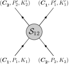
Figure 3: Scattering process and transformation of central charges.

Representation Structure.

First of all, we demand that $\mathcal{S}_{12}$ exchanges the central charges $C$ of the two involved particles

$$C^{\prime}_{1}=C_{1},\quad C^{\prime}_{2}=C_{2}.$$ (3.2)

The reason is that $C_{k}$ is interpreted as an energy of a particle and should therefore be tightly attached to it. The transformation of the other central charges is then determined by the symmetry: Firstly, the charges should add up to the same values leading to the constraints

$$P_{1}+P_{2}=P^{\prime}_{1}+P^{\prime}_{2},\qquad K_{1}+K_{2}=K^{\prime}_{1}+K^{\prime}_{2}.$$ (3.3)

Secondly, the shortening conditions must remain true, i.e.

$$P_{j}K_{j}=P^{\prime}_{j}K^{\prime}_{j}\quad\mbox{for }j=1,2.$$ (3.4)

This system of four equations has the obvious solution where also the other central charges are merely exchanged

$$P^{\prime}_{j}=P_{j},\quad K^{\prime}_{j}=K_{j}.$$ (3.5)

Due to the equations’ quadratic nature, a second solution exists where the other charges are transformed non-trivially

$$P^{\prime}_{j}=K_{j}\,\frac{P_{1}+P_{2}}{K_{1}+K_{2}}\,,\quad K^{\prime}_{j}=P_{j}\,\frac{K_{1}+K_{2}}{P_{1}+P_{2}}\,.$$ (3.6)

Uniqueness.

The degrees of freedom of an invariant operator acting on a tensor product equal the number of irreducible components in the tensor product. What is special about the fundamental representation of $\mathfrak{h}$ is that its tensor product with another fundamental contains merely one irreducible component (2.21)

$$\langle\vec{C}_{1}\rangle\otimes\langle\vec{C}_{2}\rangle=\{0,0;\vec{C}_{1}+\vec{C}_{2}\}.$$ (3.7)

Therefore the S-matrix is defined uniquely up to one overall factor.

The choice (3.5) for the representations would obviously lead to a graded permutation $\mathcal{S}_{12}\sim\mathcal{P}_{12}$ (up to an overall factor). This yields a perfectly well-defined, albeit boring S-matrix, so we shall discard this case. The other choice (3.6) leads to non-trivial results and we will only consider this case in what follows.

3.2 Chains and Factorised Scattering

Now consider a sequence of $K$ fundamental multiplets

$$\langle\vec{C}_{1}\rangle\otimes\langle\vec{C}_{2}\rangle\otimes\ldots\otimes\langle\vec{C}_{K}\rangle;$$ (3.8)

this will be called a chain. Let $\mathcal{S}_{kj}$ act on a pair of adjacent multiplets while acting as the identity on the others. Note that the labels of $\mathcal{S}$ shall always refer to the labels of the central charges $C_{k}$. After some initial permutations these will not be in proper order anymore, but in some sequence $C_{\pi(k)}$ with the overall permutation specified by $\pi$. Acting on such a state, $\mathcal{S}_{\pi(k),\pi(k+1)}$ would be a proper nearest-neighbour S-matrix.

Permutation Group.

A basic requirement for a consistent definition of a factorised $K$-particle S-matrix $\mathcal{S}_{\pi}$ for any permutation $\pi\in S_{K}$ is that it forms a representation of the permutation group $S_{K}$, i.e. $\mathcal{S}_{\pi^{\prime}}\mathcal{S}_{\pi}=\mathcal{S}_{\pi^{\prime}\pi}$. As $S_{K}$ is generated by permutations of nearest neighbours, we can always write $\mathcal{S}_{\pi}$ as a product of nearest-neighbour S-matrices $\mathcal{S}_{kj}$, i.e. the S-matrix factorises. See the example in Fig. 4. The necessary and sufficient conditions for the nearest-neighbour S-matrix $\mathcal{S}_{kj}$ to generate a representation of $S_{K}$ are (see Fig. 5) the unitarity condition

$$\mathcal{S}_{21}\mathcal{S}_{12}=\mathcal{I}$$ (3.9)

and the Yang-Baxter equation

$$\mathcal{S}_{12}\mathcal{S}_{13}\mathcal{S}_{23}=\mathcal{S}_{23}\mathcal{S}_{13}\mathcal{S}_{12}.$$ (3.10)

Together they allow to bring any product of $\mathcal{S}_{kj}$ to some standard form $\mathcal{S}_{\pi}$ depending only on the permutation $\pi\in S_{K}$.

$=$

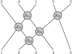
Figure 4: Factorised scattering.

$=$      $=$

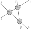
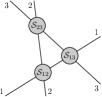
Figure 5: Unitarity condition and Yang-Baxter equation.

Labels.

Let us now focus on the representation labels: According to the definition (3.1), the action of $\mathcal{S}_{\pi}$ results in a new sequence of labels

$$\mathcal{S}_{\pi}:\langle\vec{C}_{1}\rangle\otimes\ldots\otimes\langle\vec{C}_{K}\rangle\mapsto\langle\vec{C}^{\pi}_{1}\rangle\otimes\ldots\otimes\langle\vec{C}^{\pi}_{K}\rangle$$ (3.11)

with $C^{\pi}_{k}=C_{\pi(k)}$ due to (3.2), and $P^{\pi}_{k},K^{\pi}_{k}$ are defined through repeated application of (3.6). Furthermore, the group multiplication rule $\mathcal{S}_{\pi^{\prime}}\mathcal{S}_{\pi}=\mathcal{S}_{\pi^{\prime}\pi}$ requires

$$\mathcal{S}_{\pi^{\prime}}:\langle\vec{C}^{\pi}_{1}\rangle\otimes\ldots\otimes\langle\vec{C}^{\pi}_{K}\rangle\mapsto\langle\vec{C}^{\pi^{\prime}\pi}_{1}\rangle\otimes\ldots\otimes\langle\vec{C}^{\pi^{\prime}\pi}_{K}\rangle.$$ (3.12)

It is straightforward to verify that (3.6) satisfies the relations (3.9,3.10) in terms of the representation labels and thus (3.12) holds.

Components.

Let us now consider the implications of (3.9,3.10) for the action of the S-matrix in components. For that purpose we shall denote the state with the highest weight w.r.t. one $\mathfrak{su}(2)$ of the fundamental multiplet as $\mathopen{|}\phi\mathclose{\rangle}$. The highest-weight state w.r.t. the other $\mathfrak{su}(2)$ shall be denoted as $\mathopen{|}\psi\mathclose{\rangle}$. Let us act with the S-matrix on a pair of such states. Due to their highest-weight nature it is clear that the resulting states will be of the same form,

$$\mathcal{S}_{12}\mathopen{|}\phi_{1}\phi_{2}\mathclose{\rangle}=A_{12}\mathopen{|}\phi_{2}\phi_{1}\mathclose{\rangle},\qquad\mathcal{S}_{12}\mathopen{|}\psi_{1}\psi_{2}\mathclose{\rangle}=D_{12}\mathopen{|}\psi_{2}\psi_{1}\mathclose{\rangle},$$ (3.13)

where we defined the corresponding matrix elements as $A_{12}$ and $D_{12}$. The coefficients $A_{12}$ and $D_{12}$ will be functions of the central charges $\vec{C}_{k}$. The above claim of uniqueness is that fixing $A_{12}$ also determines $D_{12}$ uniquely.

Unitarity.

Let us consider (3.9) first. As mentioned below (3.12) the unitarity condition holds in terms of representations, i.e.

$$\mathcal{S}_{21}\mathcal{S}_{12}:\langle\vec{C}_{1}\rangle\otimes\langle\vec{C}_{2}\rangle\mapsto\langle\vec{C}_{1}\rangle\otimes\langle\vec{C}_{2}\rangle.$$ (3.14)

The combination $\mathcal{S}_{21}\mathcal{S}_{12}$ is an $\mathfrak{h}$-invariant operator and for the same reasons as for $\mathcal{S}_{12}$ given around (3.7), it is uniquely defined up to an overall factor. As the identity acts like (3.14), the two maps must be proportional

$$\mathcal{S}_{21}\mathcal{S}_{12}\sim\mathcal{I}.$$ (3.15)

To find the factor of proportionality, we shall act on the state $\mathopen{|}\phi_{1}\phi_{2}\mathclose{\rangle}$ and obtain

$$\mathcal{S}_{21}\mathcal{S}_{12}\mathopen{|}\phi_{1}\phi_{2}\mathclose{\rangle}=A_{12}A_{21}\mathopen{|}\phi_{1}\phi_{2}\mathclose{\rangle}.$$ (3.16)

It implies that the relation

$$A_{12}A_{21}=1$$ (3.17)

is sufficient to ensure by $\mathfrak{h}$-symmetry that the unitarity condition (3.9) holds for the entire S-matrix. In particular this fact together with $\mathcal{S}_{21}\mathcal{S}_{12}\mathopen{|}\psi_{1}\psi_{2}\mathclose{\rangle}=D_{12}D_{21}\mathopen{|}\psi_{1}\psi_{2}\mathclose{\rangle}$ implies that the relation

$$D_{12}D_{21}=1$$ (3.18)

is equivalent to (3.17) by $\mathfrak{h}$-symmetry.

Yang-Baxter Equation.

Let us now consider the Yang-Baxter equation (3.10). By moving all the terms to one side, we can write it as

$$\mathcal{S}_{32}\mathcal{S}_{31}\mathcal{S}_{21}\mathcal{S}_{23}\mathcal{S}_{13}\mathcal{S}_{12}=\mathcal{I}.$$ (3.19)

Reminding ourselves of the tensor product (2.23)

$$\langle\vec{C}_{1}\rangle\otimes\langle\vec{C}_{2}\rangle\otimes\langle\vec{C}_{3}\rangle=\{1,0;\vec{C}_{1}+\vec{C}_{2}+\vec{C}_{3}\}\oplus\{0,1;\vec{C}_{1}+\vec{C}_{2}+\vec{C}_{3}\}$$ (3.20)

we find that it is sufficient to prove (3.19) for one state in each of the two irreducible components. The simplest such states are given by $\mathopen{|}\phi_{1}\phi_{2}\phi_{3}\mathclose{\rangle}$ and $\mathopen{|}\psi_{1}\psi_{2}\psi_{3}\mathclose{\rangle}$. For these it is straightforward to evaluate (3.10):

$$A_{\underline{23}1}A_{2\underline{13}}A_{\underline{12}3}=A_{3\underline{12}}A_{\underline{13}2}A_{1\underline{23}},\qquad D_{\underline{23}1}D_{2\underline{13}}D_{\underline{12}3}=D_{3\underline{12}}D_{\underline{13}2}D_{1\underline{23}}.$$ (3.21)

Here $A_{2\underline{13}}$ represents the element $A_{13}$ when the particles have been permuted to the sequence $213$ in the initial state before applying $\mathcal{S}_{13}$. Note that it is important to keep track of all the labels because the S-matrix is based on the relation (3.6) which changes the central charges $P,K$ non-trivially.

We can ensure that one of the equations holds by choosing a suitable function $A$ or $D$. However, the ratio of the equations depends on $A/D$ only which is determined by $\mathfrak{h}$-symmetry as explained below (3.18). We thus have to ensure

$$A_{\underline{23}1}A_{2\underline{13}}A_{\underline{12}3}=A_{3\underline{12}}A_{\underline{13}2}A_{1\underline{23}},\qquad\frac{A_{\underline{23}1}}{D_{\underline{23}1}}\,\frac{A_{2\underline{13}}}{D_{2\underline{13}}}\,\frac{A_{\underline{12}3}}{D_{\underline{12}3}}=\frac{A_{3\underline{12}}}{D_{3\underline{12}}}\,\frac{A_{\underline{13}2}}{D_{\underline{13}2}}\,\frac{A_{1\underline{23}}}{D_{1\underline{23}}}\,.$$ (3.22)

To prove them, it would suffice to ensure

$$A_{\underline{12}3}=A_{3\underline{12}}\quad\mbox{and}\quad\frac{A_{\underline{12}3}}{D_{\underline{12}3}}=\frac{A_{3\underline{12}}}{D_{3\underline{12}}}\,,$$ (3.23)

i.e. that the scattering of two highest-weight states of one $\mathfrak{su}(2)$ is independent of their position within the chain. Note that the representation labels do depend on the position, see (3.12,3.6), and therefore (3.23) is far from evident.

3.3 Constrained Labels

So far the representations labels $P_{j},K_{j}$ in the natural ordering of particles have been considered to be completely general. However, we will have to impose certain relations among the labels in order to satisfy the Yang-Baxter equation or (3.23). To see this would require a substantial amount of work involving the explicit expression for the S-matrix. Here we will present a plausible constraint related to the S-matrix bootstrap, cf. [46]. This constraint leads to strong simplifications and it will turn out to solve the YBE. We can however not determine rigorously whether the derived constraint is minimal or not.

Scattering with a Pair of Particles.

Consider the permutation $\pi$ that interchanges three modules as follows

$$\mathcal{S}_{\pi}:\langle\vec{C}_{1}\rangle\otimes\langle\vec{C}_{2}\rangle\otimes\langle\vec{C}_{3}\rangle\mapsto\langle\vec{C}^{\prime}_{3}\rangle\otimes\langle\vec{C}^{\prime}_{1}\rangle\otimes\langle\vec{C}^{\prime}_{2}\rangle.$$ (3.24)

Applying (3.6) two times we find

$$P^{\prime}_{3}=P_{3}\,\frac{P_{1}K_{2}+(P_{1}+P_{2}+P_{3})K_{3}}{K_{1}P_{2}+(K_{1}+K_{2}+K_{3})P_{3}}\,.$$ (3.25)

Alternatively, in the S-matrix bootstrap we could interpret the pair $\langle\vec{C}_{1}\rangle\otimes\langle\vec{C}_{2}\rangle$ as a composite multiplet $\{0,0;\vec{C}_{1}+\vec{C}_{2}\}$ which we scatter with $\langle\vec{C}_{3}\rangle$. While in general the long multiplet is irreducible, for particular values of $\vec{C}_{1}+\vec{C}_{2}$ it splits into two short multiplets, cf. (2.18). In that case, the analog of formula (3.6) must apply to preserve the shortness of the composite multiplet

$$P^{\prime}_{3}=K_{3}\,\frac{(P_{1}+P_{2})+P_{3}}{(K_{1}+K_{2})+K_{3}}\,.$$ (3.26)

A natural way to ensure consistency in general is to let the relation hold in general. Equating the two expressions for $P^{\prime}_{3}$, we obtain the constraint

$$\frac{P_{2}(P_{1}+P_{2}+P_{3})}{P_{1}P_{3}}=\frac{K_{2}(K_{1}+K_{2}+K_{3})}{K_{1}K_{3}}\,.$$ (3.27)

There are further ways of expressing the consequences of this constraint: First of all, it is certainly not a bad idea to have (3.6) hold also for scattering of composite objects. Secondly, the invariant $(\vec{C}_{1}+\vec{C}_{2})^{2}$ is preserved by the scattering. Thirdly, we have $P^{\prime}_{1}/P_{1}=P^{\prime}_{2}/P_{2}=K_{1}/K^{\prime}_{1}=K_{2}/K^{\prime}_{2}$; in other words $P_{1}$ and $P_{2}$ are multiplied by a common factor and $K_{1},K_{2}$ are multiplied by its inverse. And finally, it appears that the Yang-Baxter equation (3.10) can only be satisfied if (3.27) holds. To confirm this we would need the explicit form of the S-matrix which is derived only later in this section. In conclusion, the above constraint ensures that the scattering of composite objects modifies the labels of the chain in the least disruptive way.

Representation Structure.

The constraint (3.27) should hold for all neighbouring triplets which reduces the $2K$ quantities $P_{k},K_{k}$ to merely $K+2$ independent ones. The unique solution to this constraint is

$$P_{k}\mathrel{} = \mathrel{}g\alpha\left(1-\exp(+ip_{k})\right)\prod_{j=1}^{k-1}\exp(+ip_{j})\,,$$

$$K_{k}\mathrel{} = \mathrel{}\frac{g}{\alpha}\left(1-\exp(-ip_{k})\right)\prod_{j=1}^{k-1}\exp(-ip_{j})\,.$$ (3.28)

Here $g$ and $\alpha$ are global constants while the momenta $p_{k}$ are defined individually for each particle. Altogether they make up the $K+2$ independent parameters of the chain. Using the shortening condition $C_{k}^{2}-P_{k}K_{k}$ we have also obtained a dispersion relation, cf. (2.34)

$$C_{k}=\pm\sqrt{{\textstyle\frac{1}{4}}+4g^{2}\sin^{2}({\textstyle\frac{1}{2}}p_{k})}\,,$$ (3.29)

which relates the momenta $p_{k}$ to central charges $C_{k}$. Note that the charges $P_{k},K_{k}$ do not only depend on the momenta $p_{k}$ at site $k$, but also on all momenta $p_{j}$ of sites $j<k$ to the left of $k$. Conversely, the charges $C_{k}$ are defined only through the momentum $p_{k}$ at the same site.

Scattering of Chains.

Now let us consider the scattering of two composites of length $k$ and $K-k$, see Fig. 6

$$\mathcal{S}_{\pi}:\langle\vec{C}_{1}\rangle\otimes\ldots\otimes\langle\vec{C}_{k}\rangle\otimes\langle\vec{C}_{k+1}\rangle\otimes\ldots\otimes\langle\vec{C}_{K}\rangle\mapsto\langle\vec{C}^{\prime}_{k+1}\rangle\otimes\ldots\otimes\langle\vec{C}^{\prime}_{K}\rangle\otimes\langle\vec{C}^{\prime}_{1}\rangle\otimes\ldots\otimes\langle\vec{C}^{\prime}_{k}\rangle.$$ (3.30)

In other words, all the particles labelled $j=1,\ldots,k$ are moved past the particles $j=k+1,\ldots,K$. Initially the charges $\vec{C}_{k}$ are given by (3.3,3.29). The resulting central charges after the scattering process are determined by repeated application of (3.6) and read

$$\begin{array}[b]{rclcrclcl}P^{\prime}_{l}\mathrel{}&=&\mathrel{}\displaystyle P_{l}\prod_{j=k+1}^{K}\exp(+ip_{j}),&&K^{\prime}_{l}\mathrel{}&=&\mathrel{}\displaystyle K_{l}\prod_{j=k+1}^{K}\exp(-ip_{j})&&\mbox{for }l\leq k,\\[3.0pt] P^{\prime}_{l}\mathrel{}&=&\mathrel{}\displaystyle P_{l}\prod_{j=1}^{k}\exp(-ip_{j}),&&K^{\prime}_{l}\mathrel{}&=&\mathrel{}\displaystyle K_{l}\prod_{j=1}^{k}\exp(+ip_{j})&&\mbox{for }l>k.\end{array}$$ (3.31)

We see that the central charges are multiplied by the net $\exp(ip)$ of the composite they scatter with. As a consequence, the invariants $(\vec{C}_{1}+\ldots+\vec{C}_{k})^{2}$ and $(\vec{C}_{k+1}+\ldots+\vec{C}_{K})^{2}$ are not changed by the scattering. In particular it means that whenever a shortening condition applies to a subchain $1\ldots k$, it will also apply after scattering with anything else. This feature is required for consistency with the S-matrix bootstrap and fusion of particles. This shows that the constraint (3.27) between the central charges of three adjacent sites is sufficient for a consistent factorised scattering.

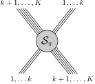
Figure 6: Scattering of two chains.

3.4 Notations

Due to (3.12) the representation labels $\vec{C}^{\pi}_{k}$ depend on the particular ordering of particles which one starts with. Furthermore, in Sec. 3.3 it became clear that $\vec{C}^{\pi}_{k}$ depends on the parameters of the individual particles in a non-local way. Here we present four different notations to deal with this complication and compare them.

Non-Local Notation.

After we apply a general permutation $\pi\in S_{K}$ to any chain of length $K$, the momenta will be redefined as follows, cf. (3.11)

$$P^{\pi}_{k}\mathrel{} = \mathrel{}g\alpha\left(1-\exp(+ip_{\pi(k)})\right)\prod_{j=1}^{k-1}\exp(+ip_{\pi(j)})\,,$$

$$K^{\pi}_{k}\mathrel{} = \mathrel{}\frac{g}{\alpha}\left(1-\exp(-ip_{\pi(k)})\right)\prod_{j=1}^{k-1}\exp(-ip_{\pi(j)})\,.$$ (3.32)

In other words, they still depend on the momenta $p_{\pi(k)}$ at site $\pi(k)$, as well as on all momenta of sites to the left. Conversely, the resulting central charges $C^{\pi}_{k}$ are just permutations of the original $C_{k}$’s

$$C^{\pi}_{k}=\pm\sqrt{{\textstyle\frac{1}{4}}+P^{\pi}_{k}K^{\pi}_{k}}\mathrel{} = \mathrel{}\pm\sqrt{{\textstyle\frac{1}{4}}+g^{2}\left(1-\exp(+ip_{\pi(k)})\right)\left(1-\exp(-ip_{\pi(k)})\right)}$$ (3.33)

$$= \mathrel{}\pm\sqrt{{\textstyle\frac{1}{4}}+4g^{2}\sin^{2}({\textstyle\frac{1}{2}}p_{\pi(k)})}=C_{\pi(k)}\,.$$

Dealing with quantities like (3.4) which do not only depend on the parameters of one site $k$, but also on the other sites $j$ and their particular ordering $\pi$ inevitably leads to a cluttering of notation. There are at least three ways to simplify the notation which we shall now present.

Cumulative Notation.

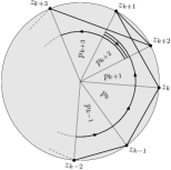
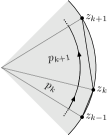
$\stackrel{{\scriptstyle\mathcal{S}_{k,k+1}}}{{\longrightarrow}}$

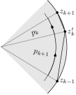
Figure 7: Cumulative picture of a chain and of a scattering process.

For the first notation based on [47] we introduce cumulative momenta $\varphi^{\pi}_{k}$ and their exponentials $z^{\pi}_{k}$ via

$$\varphi^{\pi}_{k}=-i\log\alpha+\sum_{j=1}^{k}p_{\pi(j)},\qquad z^{\pi}_{k}=\exp(i\varphi^{\pi}_{k})=\alpha\prod_{j=1}^{k}\exp(ip_{\pi(j)}).$$ (3.34)

The relation between the momenta $p$ and the $z$ parameters is best displayed pictorially in Fig. 7. These cumulative parameters allow us to write the central charges $P,K$ simply as differences

$$P^{\pi}_{k}=gz^{\pi}_{k-1}-gz^{\pi}_{k},\qquad K^{\pi}_{k}=g/z^{\pi}_{k-1}-g/z^{\pi}_{k}.$$ (3.35)

This notation is closest in nature to string theory on $AdS_{5}\times S^{5}$ using the coordinates introduced in [48]. Here the parameters $\varphi_{k}$ represent angles on a great circle of $S^{5}$. In the figure, a string excitation with momentum $p_{k}$ corresponds to the line segments joining the points $z_{k-1}$ and $z_{k}$ [47]. Conversely, the latter determine the position of the string between two excitations. Scattering of two particles $k,k+1$ is illustrated on the r.h.s. of Fig. 7. It interchanges two neighbouring line segments and consequently modifies only the intermediate point $z_{k}\mapsto z^{\prime}_{k}$. The overall central charges $P,K$ for a chain of particles are immediately determined by (3.35) as $P=gz^{\pi}_{0}-gz^{\pi}_{K}$ and $K=g/z^{\pi}_{0}-g/z^{\pi}_{K}$. As the endpoints of a chain remain fixed, $P,K$ are obviously preserved in any scattering process. Moreover, a closed chain with $z^{\pi}_{K}=z^{\pi}_{0}$ has vanishing charges $P=K=0$.

All in all, this notation gets rid of the non-local contributions but still requires to carry along the dependence on the order of particles in $\pi$. It is therefore only partially suitable to tidy up the expressions. Before proceeding to a different notation, let us make some comments:

It is curious to see that in this picture both sides of the constraint (3.27) take the form of a conformal cross ratio, cf. (3.35)

$$\frac{(z_{1}-z_{2})(z_{0}-z_{3})}{(z_{0}-z_{1})(z_{2}-z_{3})}=\frac{(1/z_{1}-1/z_{2})(1/z_{0}-1/z_{3})}{(1/z_{0}-1/z_{1})(1/z_{2}-1/z_{3})}\,.$$ (3.36)

The conformal cross ratio is invariant under inversion $z_{k}\mapsto 1/z_{k}$ showing that (3.27) follows from (3.35). It remains a question if there is a meaning to conformal transformations of this $z$-plane which map the unit circle to itself.

Finally, this notation sheds some light on the nature of the constant $\alpha$. The definition (3.34) implies $z^{\pi}_{0}=\alpha$, therefore $\alpha$ determines the origin for a chain of particles in $z$-space.

Twisted Notation.

In a different notation due to [27] we allow for certain markers $\mathcal{Z}^{n}$ to be inserted between the particles of a chain, e.g.

$$\mathopen{|}\ldots\mathcal{X}_{4}\,\mathcal{Z}^{+1}\,\mathcal{X}_{5}\mathcal{X}_{6}\,\mathcal{Z}^{-2}\,\mathcal{X}_{7}\ldots\mathclose{\rangle},$$ (3.37)

where $\mathcal{X}_{k}$ represents some state in $\langle\vec{C}_{k}\rangle$. These can be shifted around the chain by picking up phases $\exp(ip_{k})$ as follows

$$\mathopen{|}\ldots\mathcal{X}_{k}\mathcal{Z}^{n}\ldots\mathclose{\rangle}=\exp(ip_{k})^{n}\mathopen{|}\ldots\mathcal{Z}^{n}\mathcal{X}\ldots\mathclose{\rangle}.$$ (3.38)

They combine by adding their exponents $\mathcal{Z}^{n}\mathcal{Z}^{m}=\mathcal{Z}^{n+m}$. In [27] the markers represent insertion or deletion of background sites $\mathcal{Z}$ within the coordinate Bethe ansatz for planar $\mathcal{N}=4$ gauge theory. The action of $\mathfrak{P},\mathfrak{K}$ on a single multiplet can then be defined as

$$\mathfrak{P}_{k}\mathopen{|}\ldots\mathcal{X}_{k}\ldots\mathclose{\rangle}=P_{k}\mathopen{|}\ldots\mathcal{Z}^{+}\mathcal{X}_{k}\ldots\mathclose{\rangle}\,,\qquad\mathfrak{K}_{k}\mathopen{|}\ldots\mathcal{X}_{k}\ldots\mathclose{\rangle}=K_{k}\mathopen{|}\ldots\mathcal{Z}^{-}\mathcal{X}_{k}\ldots\mathclose{\rangle},$$ (3.39)

where $P_{k},K_{k}$ now only depend on the momentum $p_{k}$ of the respective site

$$P_{k}=g\alpha\left(1-\exp(+ip_{k})\right),\qquad K_{k}=\frac{g}{\alpha}\left(1-\exp(-ip_{k})\right).$$ (3.40)

Within a chain, $\mathfrak{P}$ acts as

$$\mathfrak{P}\mathopen{|}\mathcal{X}_{1}\mathcal{X}_{2}\mathcal{X}_{3}\ldots\mathclose{\rangle}\mathrel{} = \mathrel{}P_{1}\mathopen{|}\mathcal{Z}^{+}\mathcal{X}_{1}\mathcal{X}_{2}\mathcal{X}_{3}\ldots\mathclose{\rangle}+P_{2}\mathopen{|}\mathcal{X}_{1}\mathcal{Z}^{+}\mathcal{X}_{2}\mathcal{X}_{3}\ldots\mathclose{\rangle}+P_{3}\mathopen{|}\mathcal{X}_{1}\mathcal{X}_{2}\mathcal{Z}^{+}\mathcal{X}_{3}\ldots\mathclose{\rangle}+\ldots$$ (3.41)

$$= \mathrel{}\bigl{(}P_{1}+\exp(ip_{1})P_{2}+\exp(ip_{1}+ip_{2})P_{3}+\ldots\bigr{)}\mathopen{|}\mathcal{Z}^{+}\mathcal{X}_{1}\mathcal{X}_{2}\mathcal{X}_{3}\ldots\mathclose{\rangle},$$

where we have shifted the marker $\mathcal{Z}^{+}$ always to the left end of the chain. The additional factors of $\exp(ip_{k})$ supply the terms of (3.3) which are missing in (3.40). We thus obtain precisely the original picture when we ignore any marker that is at the very left of a chain. The benefit of this notation is that all the particles are completely independent of each other. The markers $\mathcal{Z}^{\pm}$ provide the missing non-local terms. By comparing (3.4) to (3.39,3.40) it should become clear how to translate between the two: For example, an insertion of $\mathcal{Z}^{+}$ leads to multiplication with $x^{+}_{j}/x^{-}_{j}$ for all particles which are to the left of particle $k$. We will thus continue to work in the twisted notation.

Hopf Algebra Notation.

Another suitable framework to deal with the above spin chain representations is given by Hopf algebras [49, 50]. This is also the standard framework for the investigation and description of integrable structures for spin chains. It is likely to play an important role for the understanding of the present integrable model, let us therefore outline the relationship to the above notation.

In the Hopf algebra one introduces a new generator $\mathfrak{U}$ which acts by returning $e^{ip}$ [49, 50]

$$\mathfrak{U}_{k}\mathopen{|}\ldots\mathcal{X}_{k}\ldots\mathclose{\rangle}=\exp(ip_{k})\mathopen{|}\ldots\mathcal{X}_{k}\ldots\mathclose{\rangle}\,.$$ (3.42)

To reproduce (3.41) one defines the action of $\mathfrak{P}$ on a chain of particles as

$$\mathfrak{P}=\sum_{j=1}^{K}\mathfrak{U}_{1}\ldots\mathfrak{U}_{j-1}\mathfrak{P}_{j}=\sum_{j=1}^{K}\mathfrak{U}^{\otimes j-1}\otimes\mathfrak{P}\otimes\mathfrak{I}^{\otimes K-j-1}.$$ (3.43)

Here $\mathfrak{I}$ is the identity operator. This representation of $\mathfrak{P}$ on the chain is easily obtained using the coproduct $\Delta:\mathfrak{h}\to\mathfrak{h}\otimes\mathfrak{h}$. For example, it acts on $\mathfrak{P}$ and $\mathfrak{U}$ as

$$\Delta\mathfrak{P}=\mathfrak{P}\otimes\mathfrak{I}+\mathfrak{U}\otimes\mathfrak{P},\qquad\Delta\mathfrak{U}=\mathfrak{U}\otimes\mathfrak{U}\,.$$ (3.44)

Then $\mathfrak{P}$ acting on the chain is simply given by the multiple coproduct $\Delta^{K-1}\mathfrak{P}$. The eigenvalue $P_{k}$ in (3.39) is obtained by setting $\mathfrak{P}=g\alpha\mathfrak{I}-g\alpha\mathfrak{U}$. Consequently, the action of $\mathfrak{P}$ on the chain yields $\Delta^{K-1}\mathfrak{P}=g\alpha\mathfrak{I}^{\otimes K}-g\alpha\mathfrak{U}^{\otimes K}$. The construction of the Hopf algebra can be extended to all generators of $\mathfrak{h}$, see [49, 50] for details and further aspects.

It is interesting to see that for the present model the representation in terms of the Lie algebra $\mathfrak{h}$ (non-local notation) coexists to the Hopf algebra representation. This is apparently related to the fact that the momentum parameters $p_{k}$ for the Hopf algebra are encoded into the representation labels $\vec{C}_{k}$ for the Lie algebra. For conventional integrable spin chains, the Lie algebra does not see the momentum parameters.

3.5 Chain of Fundamentals

We would now like to set up the action of the symmetry generators on a chain of fundamental multiplets. Here the twisted notation turns out to be very useful.

Twisted Notation.

The action of the bosonic $\mathfrak{su}(2)\times\mathfrak{su}(2)$ generators is canonical. The action of fermionic generators on each particle is as in (2.4), but with markers $\mathcal{Y},\mathcal{Z}$ inserted

$$\mathfrak{Q}^{\alpha}{}_{a}{}_{,k}\mathopen{|}\ldots\phi^{b}_{k}\ldots\mathclose{\rangle}\mathrel{} = \mathrel{}a_{k}\,\delta^{b}_{a}\mathopen{|}\ldots\mathcal{Y}^{+}\psi^{\alpha}_{k}\ldots\mathclose{\rangle},$$

$$\mathfrak{Q}^{\alpha}{}_{a}{}_{,k}\mathopen{|}\ldots\psi^{\beta}_{k}\ldots\mathclose{\rangle}\mathrel{} = \mathrel{}b_{k}\,\varepsilon^{\alpha\beta}\varepsilon_{ab}\mathopen{|}\ldots\mathcal{Z}^{+}\mathcal{Y}^{-}\phi^{b}_{k}\ldots\mathclose{\rangle},$$

$$\mathfrak{S}^{a}{}_{\alpha}{}_{,k}\mathopen{|}\ldots\phi^{b}_{k}\ldots\mathclose{\rangle}\mathrel{} = \mathrel{}c_{k}\,\varepsilon^{ab}\varepsilon_{\alpha\beta}\mathopen{|}\ldots\mathcal{Z}^{-}\mathcal{Y}^{+}\psi^{\beta}_{k}\ldots\mathclose{\rangle},$$

$$\mathfrak{S}^{a}{}_{\alpha}{}_{,k}\mathopen{|}\ldots\psi^{\beta}_{k}\ldots\mathclose{\rangle}\mathrel{} = \mathrel{}d_{k}\,\delta^{\beta}_{\alpha}\mathopen{|}\ldots\mathcal{Y}^{-}\phi^{a}_{k}\ldots\mathclose{\rangle}.$$ (3.45)

The coefficients $a_{k}$ are given in (2.29)

$$a_{k}=\sqrt{g}\,\gamma_{k},\quad b_{k}=\sqrt{g}\,\frac{\alpha}{\gamma_{k}}\left(1-\frac{x^{+}_{k}}{x^{-}_{k}}\right),\quad c_{k}=\sqrt{g}\,\frac{i\gamma_{k}}{\alpha x^{+}_{k}}\,,\quad d_{k}=\sqrt{g}\,\frac{x^{+}_{k}}{i\gamma_{k}}\left(1-\frac{x^{-}_{k}}{x^{+}_{k}}\right)$$ (3.46)

with arbitrary $g,\alpha,\gamma_{k},x^{\pm}_{k}$ subject to the constraint

$$x^{+}_{k}+\frac{1}{x^{+}_{k}}-x^{-}_{k}-\frac{1}{x^{-}_{k}}=\frac{i}{g}\,.$$ (3.47)

The action of the central charges is as follows

$$\mathfrak{C}_{k}\mathopen{|}\ldots\mathcal{X}_{k}\ldots\mathclose{\rangle}\mathrel{} = \mathrel{}C_{k}\mathopen{|}\ldots\mathcal{X}_{k}\ldots\mathclose{\rangle},$$

$$\mathfrak{P}_{k}\mathopen{|}\ldots\mathcal{X}_{k}\ldots\mathclose{\rangle}\mathrel{} = \mathrel{}P_{k}\mathopen{|}\ldots\mathcal{Z}^{+}\mathcal{X}_{k}\ldots\mathclose{\rangle},$$

$$\mathfrak{K}_{k}\mathopen{|}\ldots\mathcal{X}_{k}\ldots\mathclose{\rangle}\mathrel{} = \mathrel{}K_{k}\mathopen{|}\ldots\mathcal{Z}^{-}\mathcal{X}_{k}\ldots\mathclose{\rangle},$$ (3.48)

with

$$C_{k}=-igx^{+}_{k}+igx^{-}_{k}-\frac{1}{2}\,,\qquad P_{k}=g\alpha\left(1-\frac{x^{+}_{k}}{x^{-}_{k}}\right),\qquad K_{k}=\frac{g}{\alpha}\left(1-\frac{x^{-}_{k}}{x^{+}_{k}}\right).$$ (3.49)

The marker $\mathcal{Z}$ can be shifted around as explained above

$$\mathopen{|}\ldots\mathcal{X}_{k}\mathcal{Z}^{\pm}\ldots\mathclose{\rangle}=\frac{x^{\pm}_{k}}{x^{\mp}_{k}}\,\mathopen{|}\ldots\mathcal{Z}^{\pm}\mathcal{X}_{k}\ldots\mathclose{\rangle}$$ (3.50)

and the new marker $\mathcal{Y}$ behaves similarly

$$\mathopen{|}\ldots\mathcal{X}_{k}\mathcal{Y}^{\pm}\ldots\mathclose{\rangle}=(\xi_{k})^{\pm 1}\,\mathopen{|}\ldots\mathcal{Y}^{\pm}\mathcal{X}_{k}\ldots\mathclose{\rangle}$$ (3.51)

with some new constants $\xi_{k}$. In conclusion, the representation on the chain is specified by two global constants $g,\alpha$ as well as the local parameters $x^{\pm}_{k},\gamma_{k},\xi_{k}$ subject to (3.47).

Non-Local Notation.

Let us rewrite the above representation in terms of the non-local notation to illustrate the differences. For that we use the representation (3.5) without insertion of the markers. We define the constants $\zeta^{\pi}_{k}$ and $\eta^{\pi}_{k}$

$$\zeta^{\pi}_{k}=\alpha\prod_{j=1}^{k-1}\frac{x^{+}_{\pi(j)}}{x^{-}_{\pi(j)}}\,,\qquad\eta^{\pi}_{k}=\gamma_{\pi(k)}\prod_{j=1}^{k-1}\xi_{\pi(j)}.$$ (3.52)

The parameters $a,b,c,d$ in (2.29) are consequently given by

$$a^{\pi}_{k}\mathrel{} = \mathrel{}\sqrt{g}\,\gamma_{\pi(k)}\prod_{j=1}^{k-1}\xi_{\pi(j)},$$

$$b^{\pi}_{k}\mathrel{} = \mathrel{}\sqrt{g}\,\frac{\alpha}{\gamma_{\pi(k)}}\,\left(1-\frac{x^{+}_{\pi(k)}}{x^{-}_{\pi(k)}}\right)\prod_{j=1}^{k-1}\left(\frac{x^{+}_{\pi(j)}}{x^{-}_{\pi(j)}}\,\frac{1}{\xi_{\pi(j)}}\right),$$

$$c^{\pi}_{k}\mathrel{} = \mathrel{}\sqrt{g}\,\frac{i\gamma_{\pi(k)}}{\alpha x^{+}_{\pi(k)}}\prod_{j=1}^{k-1}\left(\frac{x^{-}_{\pi(j)}}{x^{+}_{\pi(j)}}\,\xi_{\pi(j)}\right),$$

$$d^{\pi}_{k}\mathrel{} = \mathrel{}\sqrt{g}\,\frac{x^{+}_{\pi(k)}}{i\gamma_{\pi(k)}}\,\left(1-\frac{x^{-}_{\pi(k)}}{x^{+}_{\pi(k)}}\right)\prod_{j=1}^{k-1}\frac{1}{\xi_{\pi(j)}}\,.$$ (3.53)

We see that this agrees with (3.46) when we take the action of the markers in (3.50,3.51) into account. This shows how much leaner than the twisted notation is in comparison to the non-local one.

3.6 Components of the S-Matrix

$$\mathcal{S}_{12}\mathopen{|}\phi_{1}^{a}\phi_{2}^{b}\mathclose{\rangle}\mathrel{} = \mathrel{}A_{12}\mathopen{|}\phi_{2}^{\{a}\phi_{1}^{b\}}\mathclose{\rangle}+B_{12}\mathopen{|}\phi_{2}^{[a}\phi_{1}^{b]}\mathclose{\rangle}+{\textstyle\frac{1}{2}}C_{12}\varepsilon^{ab}\varepsilon_{\alpha\beta}\mathopen{|}\mathcal{Z}^{-}\mathcal{Y}^{+}\mathcal{Y}^{+}\psi_{2}^{\alpha}\psi_{1}^{\beta}\mathclose{\rangle},$$

$$\mathcal{S}_{12}\mathopen{|}\psi_{1}^{\alpha}\psi_{2}^{\beta}\mathclose{\rangle}\mathrel{} = \mathrel{}D_{12}\mathopen{|}\psi_{2}^{\{\alpha}\psi_{1}^{\beta\}}\mathclose{\rangle}+E_{12}\mathopen{|}\psi_{2}^{[\alpha}\psi_{1}^{\beta]}\mathclose{\rangle}+{\textstyle\frac{1}{2}}F_{12}\varepsilon^{\alpha\beta}\varepsilon_{ab}\mathopen{|}\mathcal{Z}^{+}\mathcal{Y}^{-}\mathcal{Y}^{-}\phi_{2}^{a}\phi_{1}^{b}\mathclose{\rangle},$$

$$\mathcal{S}_{12}\mathopen{|}\phi_{1}^{a}\psi_{2}^{\beta}\mathclose{\rangle}\mathrel{} = \mathrel{}G_{12}\mathopen{|}\psi_{2}^{\beta}\phi_{1}^{a}\mathclose{\rangle}+H_{12}\mathopen{|}\phi_{2}^{a}\psi_{1}^{\beta}\mathclose{\rangle},$$

$$\mathcal{S}_{12}\mathopen{|}\psi_{1}^{\alpha}\phi_{2}^{b}\mathclose{\rangle}\mathrel{} = \mathrel{}K_{12}\mathopen{|}\psi_{2}^{\alpha}\phi_{1}^{b}\mathclose{\rangle}+L_{12}\mathopen{|}\phi_{2}^{b}\psi_{1}^{\alpha}\mathclose{\rangle}.$$

$$A_{12}\mathrel{} = \mathrel{}S^{0}_{12}\,\frac{x^{+}_{2}-x^{-}_{1}}{x^{-}_{2}-x^{+}_{1}}\,,$$

$$B_{12}\mathrel{} = \mathrel{}S^{0}_{12}\,\frac{x^{+}_{2}-x^{-}_{1}}{x^{-}_{2}-x^{+}_{1}}\left(1-2\,\frac{1-1/x^{-}_{2}x^{+}_{1}}{1-1/x^{+}_{2}x^{+}_{1}}\,\frac{x^{-}_{2}-x^{-}_{1}}{x^{+}_{2}-x^{-}_{1}}\right),$$

$$C_{12}\mathrel{} = \mathrel{}S^{0}_{12}\,\frac{2\gamma_{1}\gamma_{2}\xi_{2}}{\alpha x^{+}_{1}x^{+}_{2}}\,\frac{1}{1-1/x^{+}_{1}x^{+}_{2}}\,\frac{x^{-}_{2}-x^{-}_{1}}{x^{-}_{2}-x^{+}_{1}}\,,$$

$$D_{12}\mathrel{} = \mathrel{}-S^{0}_{12}\,\frac{\xi_{2}}{\xi_{1}}\,,$$

$$E_{12}\mathrel{} = \mathrel{}-S^{0}_{12}\,\frac{\xi_{2}}{\xi_{1}}\left(1-2\,\frac{1-1/x^{+}_{2}x^{-}_{1}}{1-1/x^{-}_{2}x^{-}_{1}}\,\frac{x^{+}_{2}-x^{+}_{1}}{x^{-}_{2}-x^{+}_{1}}\right),$$

$$F_{12}\mathrel{} = \mathrel{}-S^{0}_{12}\,\frac{2\alpha(x^{+}_{1}-x^{-}_{1})(x^{+}_{2}-x^{-}_{2})}{\gamma_{1}\gamma_{2}\xi_{1}x^{-}_{1}x^{-}_{2}}\,\frac{1}{1-1/x^{-}_{1}x^{-}_{2}}\,\frac{x^{+}_{2}-x^{+}_{1}}{x^{-}_{2}-x^{+}_{1}}\,,$$

$$G_{12}\mathrel{} = \mathrel{}S^{0}_{12}\,\frac{1}{\xi_{1}}\frac{x^{+}_{2}-x^{+}_{1}}{x^{-}_{2}-x^{+}_{1}}\,,$$

$$H_{12}\mathrel{} = \mathrel{}S^{0}_{12}\,\frac{\gamma_{1}\xi_{2}}{\gamma_{2}\xi_{1}}\,\frac{x^{+}_{2}-x^{-}_{2}}{x^{-}_{2}-x^{+}_{1}}\,,$$

$$K_{12}\mathrel{} = \mathrel{}S^{0}_{12}\,\frac{\gamma_{2}}{\gamma_{1}}\,\frac{x^{+}_{1}-x^{-}_{1}}{x^{-}_{2}-x^{+}_{1}}\,,$$

$$L_{12}\mathrel{} = \mathrel{}S^{0}_{12}\,\xi_{2}\,\frac{x^{-}_{2}-x^{-}_{1}}{x^{-}_{2}-x^{+}_{1}}\,.$$

Table 1: The fundamental S-matrix of $\mathfrak{h}$.

We can now solve for the S-matrix by demanding its invariance under $\mathfrak{h}$

$$[\mathfrak{J_{1}}+\mathfrak{J_{2}},\mathcal{S}_{12}]=0.$$ (3.54)

As discussed above this will lead to a unique result up to one overall phase factor $S^{0}_{12}$. The results are summarised in Tab. 1. The expressions are slightly more general than the ones found in [27] due to the introduction of the marker $\mathcal{Y}^{\pm}$, but otherwise they agree.

Factorised Scattering.

We can now confirm unitarity and the Yang-Baxter equation. First of all (3.17) implies a constraint for the overall phase factor

$$S^{0}_{12}S^{0}_{21}=1.$$ (3.55)

Furthermore, we see that

$$A_{12}=S^{0}_{12}\,\frac{x^{+}_{2}-x^{-}_{1}}{x^{-}_{2}-x^{+}_{1}}\,,\qquad\frac{A_{12}}{D_{12}}=-\frac{\xi_{1}}{\xi_{2}}\,\frac{x^{+}_{2}-x^{-}_{1}}{x^{-}_{2}-x^{+}_{1}}$$ (3.56)

depend only on the parameters of sites $1,2$. Therefore the YBE is proved via (3.23).

Note that for two sites the choice made in Sec. 3.3 is not a restriction but fully general. There are four independent new parameters $\alpha,g,x^{+}_{1},x^{+}_{2}$ to replace the original independent charges $P_{1},P_{2},K_{1},K_{2}$. Thus we could use the expression in Tab. 1 to investigate the YBE in the more general case. Nevertheless we should emphasise that all of $\alpha,g,x^{\pm}_{1},x^{\pm}_{2}$ will become dependent not only on the site, but also on the permutation of sites. This will make the investigation of the YBE, even in the simplified form (3.22), quite hard.

Non-Local Notation.

Curiously, the markers $\mathcal{Z}^{\pm}$ and $\mathcal{Y}^{\pm}$ appear only for the contributions with coefficients $C_{12}$ and $F_{12}$ and even in the same combination. Here it is worth emphasising that in the non-local notation the insertions of $\mathcal{Z}^{-}\mathcal{Y}^{+}\mathcal{Y}^{+}$ would lead to an additional factor of

$$\prod_{j=1}^{k-1}\left(\frac{x^{-}_{\pi(j)}}{x^{+}_{\pi(j)}}\,(\xi_{\pi(j)})^{2}\right)$$ (3.57)

in $C_{12}$ when the S-matrix is applied to position $k,k+1$ of the chain. Likewise $\mathcal{Z}^{+}\mathcal{Y}^{-}\mathcal{Y}^{-}$ leads to the inverse of (3.57) as an additional factor in $F_{12}$. To complete the non-local notation, all symbols $x^{\pm}_{j},\gamma_{j},\xi_{j}$ with $j=1,2$ in Tab. 1 will have to be replaced by the symbols $x^{\pm}_{\pi(k+j-1)},\gamma_{\pi(k+j-1)},\xi_{\pi(k+j-1)}$, respectively.

3.7 Crossing Symmetry

Figure 8: S-matrix and crossed S-matrix.

S-matrices of integrable models are commonly expected to obey crossing relations. Crossing of the S-matrix replaces one particle with its conjugate particle propagating backwards in space and time, see Fig. 8. The kinematic parameters of the conjugate particle are obtained by the antipode map

$$x^{\pm}_{k}\mapsto x^{\pm}_{\bar{k}}=1/x^{\pm}_{k}.$$ (3.58)

In [30] the condition for a crossing-symmetric S-matrix was derived to be

$$X_{12}=1,$$ (3.59)

where $X_{12}=X(x^{\pm}_{1},x^{\pm}_{2})$ is a function depending on the phase factor $S^{0}_{12}$

$$X_{12}=\frac{S^{0}_{1\bar{2}}S^{0}_{12}}{\xi_{1}^{2}}\,\frac{x^{+}_{2}-x^{-}_{1}}{x^{-}_{2}-x^{-}_{1}}\,\frac{1/x^{+}_{2}-x^{+}_{1}}{1/x^{-}_{2}-x^{+}_{1}}\,.$$ (3.60)

Here $S^{0}_{1\bar{2}}$ denotes the crossed phase factor $S^{0}_{1\bar{2}}=S^{0}(x^{\pm}_{1},1/x^{\pm}_{2})$. A naive attempt to solve the crossing relation by finding a suitable phase factor $S^{0}_{12}$ must fail: If $X_{12}=1$ holds, then also $X_{1\bar{2}}=X(x^{\pm}_{1},1/x^{\pm}_{2})=1$ must be true. However, both equations are incompatible because $X_{12}/X_{1\bar{2}}$ is independent of $S^{0}_{12}$ and does not equal unity. The resolution to this problem is to allow branch cuts in the function $S^{0}_{12}$. Then the antipode map $x^{\pm}\mapsto 1/x^{\pm}$ is not an involution when applied to the phase factor. The doubled map $x^{\pm}\mapsto 1/x^{\pm}\mapsto x^{\pm}$ should instead correspond to change of Riemann sheets in the function $S^{0}_{12}$.

Indeed, the leading orders of the function $S^{0}_{12}$ extracted from perturbative string theory [15, 51, 52, 53] do have branch cuts and are consistent with the crossing relation [54, 31]. Therefore it is natural to expect crossing symmetry to hold exactly. A crossing-symmetric phase for perturbative $AdS_{5}\times S^{5}$ string theory was proposed recently in [32].

In this article we shall not assume that the phase factor satisfies the crossing equation $X_{kj}=1$. In this way we avoid having to deal with an intricate analytic structure involving multiple Riemann sheets, see [54, 31, 32]. Nevertheless, it is worth keeping in mind that occurrences of $X_{kj}$ may be set to $1$ in a crossing-symmetric model.

3.8 Special Points and Bootstrap

Let us briefly study special points of the S-matrix and relate them to the structure of representations.

Identity.

When the particle momenta become equal,

$$x^{\pm}_{2}=x^{\pm}_{1},$$ (3.61)

the S-matrix degenerates into a permutation operator with negative sign. It interchanges the particles without interchanging their flavours

$$\mathcal{S}_{12}\mathopen{|}\mathcal{X}_{1}\mathcal{X}^{\prime}_{2}\mathclose{\rangle}=-\mathopen{|}\mathcal{X}_{2}\mathcal{X}^{\prime}_{1}\mathclose{\rangle}.$$ (3.62)

It also inverts the sign. Essentially, as the particle representations are equal, it acts like the identity $\mathcal{S}_{12}=-\mathcal{I}_{12}$, it merely interchanges the particle labels.

Symmetric Products.

It is straightforward to see that for

$$x^{+}_{2}=x^{-}_{1}$$ (3.63)

the coefficient $A_{12}$ in Tab. 1 is zero. Also several other combinations of coefficients vanish. Therefore, at this point, $\mathcal{S}_{12}$ becomes a projector. This feature is related to the multiplet splitting rule (2.18). In general, two sites together form a long multiplet $\{0,0;\vec{C}\}$. However, if $\vec{C}^{2}=1$, this multiplet splits up into two short multiplets

$$\{0,0;\vec{C}\}=\langle 1,0;\vec{C}\rangle\oplus\langle 0,1;\vec{C}\rangle.$$ (3.64)

As noted in [55], the condition $\vec{C}^{2}=1$ is met when (3.63) holds. At this point, the scattering matrix projects out the first of these multiplets (symmetric product) and leaves only the latter (antisymmetric product). Likewise, if instead

$$x^{-}_{2}=x^{+}_{1},$$ (3.65)

the S-matrix becomes a projector, but onto the other irreducible multiplet (symmetric product).

Higher Representations.

The projective character of the S-matrix can be used to construct the S-matrix for various tensor product representations. One merely has to prepare composite states which transform in the desired representation and then scatter them as a whole with other objects, see Fig. 6. In particular, by chaining up particles with $x^{\pm}_{k}=x^{\mp}_{k+1}$ one obtains the totally symmetric representations $\langle m,0\rangle$ in (2.12). These composite states are also called bound states, cf. [55].

Adjoint and Singlet.

Another interesting point is

$$x^{\pm}_{2}=1/x^{\pm}_{1}.$$ (3.66)

Here, all central charges vanish, $\vec{C}=0$, and the long multiplet $\{0,0;\vec{C}\}$ splits up into a singlet and an adjoint. Poles can be observed in $B_{12},C_{12},E_{12},F_{12}$ and it would be necessary to investigate the action of $\mathcal{S}_{12}$ further. Here, some complications arise due to the semi-reducible nature of the adjoint representation in $\mathfrak{u}(N|N)$ algebras.

The singlet state however may be constructed easily, see [27]. Here it takes the form

$$\mathopen{|}{\mathbf{1}}_{12}\mathclose{\rangle}=\frac{\alpha}{\gamma_{1}\gamma_{2}\xi_{1}}\left(\frac{x^{+}_{1}}{x^{-}_{1}}-1\right)\varepsilon_{ab}\mathopen{|}\mathcal{Y}^{-}\mathcal{Y}^{-}\mathcal{Z}^{+}\phi^{a}_{1}\phi^{b}_{2}\mathclose{\rangle}+\varepsilon_{\alpha\beta}\mathopen{|}\psi^{\alpha}_{1}\psi^{\beta}_{2}\mathclose{\rangle}$$ (3.67)

where $x^{\pm}_{1}=1/x^{\pm}_{2}$. This composite has vanishing central charges, however the constituents have non-zero central charges. When we flip space, time and $\mathfrak{su}(2)$ charges for particle $1$, then it becomes equivalent to particle $2$, i.e. the two constituents are CPT-conjugates. On l.h.s. of Fig. 9, particle $1$ can be viewed as the part of the worldline of particle $2$ which moves backwards in time. We can thus view the singlet state as a curl of the worldline of particle $2$ moving backwards in time for a while. In other words, one might consider the singlet as a particle-hole fluctuation of the vacuum.

$=$

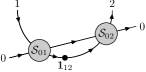
Figure 9: Singlet state and relation for trivial scattering.

Let us now scatter the singlet state with an arbitrary site $\mathcal{X}_{0}$. We find [27]

$$\mathcal{S}_{02}\mathcal{S}_{01}\,\mathopen{|}\mathcal{X}_{0}{\mathbf{1}}_{12}\mathclose{\rangle}=X_{0,12}\,\mathopen{|}{\mathbf{1}}_{12}\mathcal{X}_{0}\mathclose{\rangle}$$ (3.68)

with the unique factor

$$X_{0,12}=\frac{S^{0}_{01}S^{0}_{02}}{\xi_{0}^{2}}\,\frac{x^{+}_{0}-x^{+}_{1}}{x^{+}_{0}-x^{-}_{1}}\,\frac{x^{-}_{0}-x^{+}_{2}}{x^{-}_{0}-x^{-}_{2}}\,.$$ (3.69)

Recalling that $x^{\pm}_{1}=1/x^{\pm}_{2}$, we observe that the function $X_{0,12}=X_{02}$ is the same as the one encountered for crossing symmetry in [30], see Sec. 3.7.

This observation can be understood diagrammatically using the r.h.s. of Fig. 9: Both arrows on $\mathcal{S}_{01}$ come from the left as for the crossed S-matrix in Fig. 8 and not from the bottom as usual. If we assume crossing symmetry to hold, then the equation in Fig. 9 is equivalent to the unitarity condition in Fig. 5 rotated by $90^{\circ}$. Therefore, we should expect the equation in Fig. 9 to hold if and only if the S-matrix is crossing-symmetric.

The crossing relation $X_{12}=1$ can now be interpreted alternatively as a bootstrap condition: The singlet state is a bound state of two particles with zero total energy and momentum. As argued above, it represents an inessential vacuum fluctuation. Therefore one may expect its scattering with any real particle to be trivial.

3.9 Diagonalisation of the S-Matrix

The diagonalisation of a slightly restricted version of the S-matrix with $\xi_{k}=1$ was performed in [27]. Let us merely highlight the differences due to the introduction of non-trivial $\xi_{k}$’s here as compared to App. C of [27].

Vacuum.

The level-II vacuum is composed from only $\phi^{1}$’s.

$$\mathopen{|}0\mathclose{\rangle}^{\mathrm{II}}=\mathopen{|}\phi^{1}_{1}\ldots\phi^{1}_{K}\mathclose{\rangle}.$$ (3.70)

Excitations.

We create an excitation $\psi^{\alpha}_{k}$ at site $k$ by acting with $(\mathfrak{Q}^{\alpha}{}_{1})_{k}$. Let us define

$$(\mathfrak{Q}^{\alpha}{}_{1})^{\pm}_{k}=\frac{x^{\mp}_{k}}{x^{\mp}_{k}-x^{\pm}_{k}}\,(\mathfrak{Q}^{\alpha}{}_{1})_{k}.$$ (3.71)

Then a level-II excitation has the following form

$$\mathopen{|}\psi^{\alpha}\mathclose{\rangle}=\sum_{k=0}^{K}\mathnormal{\Psi}_{k}(y)\bigl{(}(\mathfrak{Q}^{\alpha}{}_{1})^{-}_{k}+(\mathfrak{Q}^{\alpha}{}_{1})^{+}_{k+1}\bigr{)}\mathopen{|}0\mathclose{\rangle}^{\mathrm{II}}$$ (3.72)

with the wave function

$$\mathnormal{\Psi}_{k}(y)=\prod_{j=1}^{k}S^{\mathrm{II,I}}(y,x_{j}).$$ (3.73)

The element $S^{\mathrm{II,I}}(y,x_{k})$ of the diagonalised S-matrix in our case is

$$S^{\mathrm{II,I}}(y,x_{k})=\xi_{k}\frac{y-x^{-}_{k}}{y-x^{+}_{k}}\,.$$ (3.74)

By comparing to (4.10) in [27], it is easy to see that the additional factor of $1/\xi_{1}$ in $G_{12}$ requires the compensating factor $\xi_{1}$ in $S^{\mathrm{II,I}}(y,x_{1})$.

Scattering.

A closer look at the first line in (4.17) of [27] shows that there must be an overall factor of $\xi_{1}$ from $S^{\mathrm{II,I}}(y_{2},x_{1})$ in the state $\mathopen{|}\psi^{\alpha}_{1}\psi^{\beta}_{2}\mathclose{\rangle}^{\mathrm{II}}$. Application of $\mathcal{S}_{12}$ to the state will then turn the factor $\xi_{1}$ into $\xi_{2}$ as desired. Consequently, the fourth and fifth lines must have the same overall factor coming from $S^{\mathrm{II,I}}(y_{1},x_{1})$. The matrix elements $M,N$ of the level-II scattering matrix thus remain unchanged. The same holds for the diagonalised elements $S^{\mathrm{II,II}}(y_{1},y_{2})$, $S^{\mathrm{III,II}}(w_{1},y_{2})$ and $S^{\mathrm{III,III}}(w_{1},w_{2})$.

Further Twisting.

In fact, we could consider a slightly generalised setup, where we introduce two more markers which rescale $\phi^{2}$ w.r.t. $\phi^{1}$ and $\psi^{2}$ w.r.t. $\psi^{1}$. These would thus break the two $\mathfrak{su}(2)$ invariances. The mechanism is the same as for $\mathcal{Y}$ which rescales $\psi^{\alpha}$ w.r.t. $\phi^{a}$ and which twists supersymmetry. It is not difficult to convince oneself that this leads to the non-trivial element of the diagonalised S-matrix

$$S^{\mathrm{III,I}}(w_{1},x_{2})=\rho_{2}$$ (3.75)

with $\rho_{k}$ determining the shift rule for the marker as in (3.51). Although we had two independent rescalings, there is only one new coefficient. This is because the spin excitation $\phi^{1}\to\phi^{2}$ is a double excitation and therefore does not come along with an independent rescaling. It should be thought of as composed from two type-II, one type-III as well as a $\mathcal{Z}^{-}$ excitation. The corresponding factor $\rho^{\prime}$ for rescaling $\phi^{2}$ w.r.t. $\phi^{1}$ must equal

$$\rho^{\prime}_{j}=\rho_{j}\xi_{j}^{2}\,\frac{x^{-}_{j}}{x^{+}_{j}}\,,$$ (3.76)

for self-consistency. Effectively, this means that we cannot have full manifest $\mathfrak{h}$-symmetry at the local level. It may nevertheless still appear as a global symmetry.

Similarly, we can twist level-II w.r.t. level-III with a global parameter $\tau$, see e.g. [56]. This introduces a factor of $\tau$ in the element $S^{\mathrm{III,II}}(w_{1},y_{2})$.

Elements.

In conclusion, the elements of the diagonalised S-matrix are given by

$$S^{\mathrm{I,0}}(x^{\pm}_{1},\cdot)\mathrel{} = \mathrel{}\frac{x^{+}_{1}}{x^{-}_{1}}\,,$$

$$S^{\mathrm{I,I}}(x^{\pm}_{1},x^{\pm}_{2})\mathrel{} = \mathrel{}S^{0}(x_{1},x_{2})\,\frac{x^{-}_{1}-x^{+}_{2}}{x^{+}_{1}-x^{-}_{2}}\,,$$

$$S^{\mathrm{II,I}}(y_{1},x^{\pm}_{2})\mathrel{} = \mathrel{}\xi_{2}\,\frac{y_{1}-x^{-}_{2}}{y_{1}-x^{+}_{2}}\,,$$

$$S^{\mathrm{II,II}}(y_{1},y_{2})\mathrel{} = \mathrel{}1,$$

$$S^{\mathrm{III,I}}(w_{1},x^{\pm}_{2})\mathrel{} = \mathrel{}\rho_{2},$$

$$S^{\mathrm{III,II}}(w_{1},y_{2})\mathrel{} = \mathrel{}\tau\,\frac{w_{1}-y_{2}-1/y_{2}-{\textstyle\frac{i}{2}}g^{-1}}{w_{1}-y_{2}-1/y_{2}+{\textstyle\frac{i}{2}}g^{-1}}\,,$$

$$S^{\mathrm{III,III}}(w_{1},w_{2})\mathrel{} = \mathrel{}\frac{w_{1}-w_{2}+ig^{-1}}{w_{1}-w_{2}-ig^{-1}}\,.$$ (3.77)

Note that $\rho_{j}$ and $\tau$ are the constants introduced above. Furthermore, the function $X_{12}$ in (3.60) related to crossing symmetry is modified to

$$X_{12}=\frac{S^{0}_{1\bar{2}}S^{0}_{12}}{\rho_{1}\xi_{1}^{2}}\,\frac{x^{+}_{2}-x^{-}_{1}}{x^{-}_{2}-x^{-}_{1}}\,\frac{1/x^{+}_{2}-x^{+}_{1}}{1/x^{-}_{2}-x^{+}_{1}}\,.$$ (3.78)

3.10 Periodic States

So far, we have been interested in chains with two ends and unspecified boundary conditions. Therefore all states made up of an arbitrary number of excitations with arbitrary momenta correspond to well-defined wave functions. If we however restrict to periodic boundary conditions, the wave function must be compatible with this periodicity. Periodicity is ensured by the Bethe equations.

Bethe Equations.

Periodicity means that the total phase factor acquired by moving any excitation by one period must be trivial, cf. Fig. 10. This condition introduces one equation per particle momentum and consequently leads to a discrete spectrum as expected for a compact space.

$=$

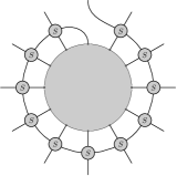
Figure 10: Bethe equations.

The scattering matrix is already in a diagonal form, so the Bethe equations for our model can be read off directly from the diagonalised elements (3.9). The Bethe equations for levels II and III read as follows, cf. [16]

$$1\mathrel{} = \mathrel{}\prod_{j=1}^{K}\frac{1}{\xi_{j}}\prod_{j=1}^{K}\frac{y_{k}-x^{+}_{j}}{y_{k}-x^{-}_{j}}\prod_{j=1}^{M}\tau\,\frac{y_{k}+1/y_{k}-w_{j}+{\textstyle\frac{i}{2}}g^{-1}}{y_{k}+1/y_{k}-w_{j}-{\textstyle\frac{i}{2}}g^{-1}}\,,$$

$$1\mathrel{} = \mathrel{}\prod_{j=1}^{K}\frac{1}{\rho_{j}}\prod_{j=1}^{N}\frac{1}{\tau}\,\frac{w_{k}-y_{j}-1/y_{j}+{\textstyle\frac{i}{2}}g^{-1}}{w_{k}-y_{j}-1/y_{j}-{\textstyle\frac{i}{2}}g^{-1}}\mathop{\prod_{j=1}^{M}}_{j\neq k}\frac{w_{k}-w_{j}-ig^{-1}}{w_{k}-w_{j}+ig^{-1}}\,.$$ (3.79)

Here $K$ is the number of sites and $N,M$ are the number of level-II and level-III excitations, respectively. Note that the individual values of $\xi_{j},\rho_{j}$ are completely irrelevant as they should because they merely represent rescalings of various types of spin orientations at different positions of the chain. However, for the Bethe equations it does matter how the spin orientations are periodically identified. This is determined by the product of all $\xi_{j}$’s and $\rho_{j}$’s, respectively.

The Bethe equations (3.10) are somewhat reminiscent of the equations for a model with $\mathfrak{su}(2|1)=\mathfrak{osp}(2|2)$ symmetry [57, 58, 59]. This is not surprising as there is a manifestly $\mathfrak{su}(2|1)$-symmetric formulation of the S-matrix and the Bethe ansatz [27]. Potentially the equations can even be matched precisely. This would require to relate the charge parameter of the four-dimensional spin representation to the spectral parameter in a special way along the lines of [60].

Dualisation.

We can perform a dualisation or particle-hole transformation on the fermionic roots $y_{j}$ [61, 62, 63, 64]: The Bethe equation for $y_{k}$ in (3.10) is in fact an algebraic equation in $y$ with coefficients independent of the $y_{j}$’s. Therefore, the $N$ parameters $y_{j}$ are the roots of this equation and there exist further $\tilde{N}$ roots $\tilde{y}_{j}$ with

$$\tilde{N}=K+2M-N.$$ (3.80)

We can reformulate this condition in terms of the function

$$Q(y)\mathrel{} = \mathrel{}\prod_{j=1}^{K}\xi_{j}\left(y-x^{-}_{j}\right)\prod_{j=1}^{N}\frac{1}{y-y_{j}}\prod_{j=1}^{\tilde{N}}\frac{1}{y-\tilde{y}_{j}}\prod_{j=1}^{M}\frac{y}{\tau}\left(y+1/y-w_{j}-{\textstyle\frac{i}{2}}g^{-1}\right)$$ (3.81)

$$\mathord{}-\prod_{j=1}^{K}\left(y-x^{+}_{j}\right)\prod_{j=1}^{N}\frac{1}{y-y_{j}}\prod_{j=1}^{\tilde{N}}\frac{1}{y-\tilde{y}_{j}}\prod_{j=1}^{M}y\left(y+1/y-w_{j}+{\textstyle\frac{i}{2}}g^{-1}\right)$$

$$= \mathrel{}\prod_{j=1}^{K}\xi_{j}\prod_{j=1}^{M}\frac{1}{\tau}-1.$$

Demanding that $Q(y)$ is constant is equivalent to the Bethe equations for the $y$’s and the $\tilde{y}$’s (which obey the same Bethe equation).

The property can be translated into a number of useful relations. In particular we find

$$\frac{Q(x^{+}_{k})}{Q(x^{-}_{k})}=\xi_{k}\,\mathop{\prod_{j=1}^{K}}_{j\neq k}\xi_{j}\,\frac{x^{+}_{k}-x^{-}_{j}}{x^{-}_{k}-x^{+}_{j}}\prod_{j=1}^{N}\frac{x^{-}_{k}-y_{j}}{x^{+}_{k}-y_{j}}\prod_{j=1}^{\tilde{N}}\frac{x^{-}_{k}-\tilde{y}_{j}}{x^{+}_{k}-\tilde{y}_{j}}\prod_{j=1}^{M}\frac{x^{+}_{k}}{\tau x^{-}_{k}}=1$$ (3.82)

and, when setting $x^{\pm}_{w_{k}}+1/x^{\pm}_{w_{k}}=w_{k}\pm i/2g$, we further obtain

$$\frac{Q(x^{+}_{w_{k}})\,Q(1/x^{+}_{w_{k}})}{Q(x^{-}_{w_{k}})\,Q(1/x^{-}_{w_{k}})}\mathrel{} = \mathrel{}\prod_{j=1}^{K}\frac{1}{\xi_{j}^{2}\tau}\,\frac{x^{+}_{j}}{x^{-}_{j}}\prod_{j=1}^{N}\tau\,\frac{w_{k}-y_{j}-1/y_{j}-{\textstyle\frac{i}{2}}g^{-1}}{w_{k}-y_{j}-1/y_{j}+{\textstyle\frac{i}{2}}g^{-1}}$$

$$\mathord{}\times\prod_{j=1}^{\tilde{N}}\tau\,\frac{w_{k}-\tilde{y}_{j}-1/\tilde{y}_{j}-{\textstyle\frac{i}{2}}g^{-1}}{w_{k}-\tilde{y}_{j}-1/\tilde{y}_{j}+{\textstyle\frac{i}{2}}g^{-1}}\mathop{\prod_{j=1}^{M}}_{j\neq k}\left(\frac{w_{k}-w_{j}+ig^{-1}}{w_{k}-w_{j}-ig^{-1}}\right)^{2}=1.$$

By using the second identity, the Bethe equations can now be written in a dual form [16],

$$1\mathrel{} = \mathrel{}\prod_{j=1}^{K}\xi_{j}\prod_{j=1}^{K}\frac{\tilde{y}_{k}-x^{-}_{j}}{\tilde{y}_{k}-x^{+}_{j}}\prod_{j=1}^{M}\frac{1}{\tau}\,\frac{\tilde{y}_{k}+1/\tilde{y}_{k}-w_{j}-{\textstyle\frac{i}{2}}g^{-1}}{\tilde{y}_{k}+1/\tilde{y}_{k}-w_{j}+{\textstyle\frac{i}{2}}g^{-1}}\,,$$

$$1\mathrel{} = \mathrel{}\prod_{j=1}^{K}\frac{1}{\rho_{j}\xi_{j}^{2}\tau}\,\frac{x^{+}_{j}}{x^{-}_{j}}\prod_{j=1}^{\tilde{N}}\tau\,\frac{w_{k}-\tilde{y}_{j}-1/\tilde{y}_{j}-{\textstyle\frac{i}{2}}g^{-1}}{w_{k}-\tilde{y}_{j}-1/\tilde{y}_{j}+{\textstyle\frac{i}{2}}g^{-1}}\mathop{\prod_{j=1}^{M}}_{j\neq k}\frac{w_{k}-w_{j}+ig^{-1}}{w_{k}-w_{j}-ig^{-1}}\,.$$ (3.84)

Symmetries.

Non-Abelian symmetries are realised in the Bethe equations by the possibility of adding Bethe roots at special points without changing the equations. These correspond to positive roots of the symmetry algebra $\mathfrak{h}$. Possible points are $y=\infty,y=0,w=\infty$ and certain combinations of these. First of all the Bethe equations for the existing roots will receive factors of $\tau$ for the introduction of new roots. This requires $\tau=1$ in order for any generator of $\mathfrak{h}$ to be preserved. Let us therefore assume $\tau=1$ in the below.

Invariance under the two $\mathfrak{su}(2)$ raising operators represented by the sets of Bethe roots $\{w=\infty\}$ and $\{w=\infty,y=\infty,y=0\}$ requires, respectively

$$\mbox{1:}\quad 1=\prod_{j=1}^{K}\rho_{j}\qquad\mbox{and}\qquad\mbox{2:}\quad 1=\prod_{j=1}^{K}\rho_{j}\xi_{j}^{2}\,\frac{x^{-}_{j}}{x^{+}_{j}}\,.$$ (3.85)

Invariance under the four fermionic raising generators requires

$$\mbox{a:}\quad 1=\prod_{j=1}^{K}\xi_{j},\qquad\mbox{b:}\quad 1=\prod_{j=1}^{K}\rho_{j}\xi_{j},\qquad\mbox{c:}\quad 1=\prod_{j=1}^{K}\xi_{j}\,\frac{x^{-}_{j}}{x^{+}_{j}}\,,\qquad\mbox{d:}\quad 1=\prod_{j=1}^{K}\rho_{j}\xi_{j}\,\frac{x^{-}_{j}}{x^{+}_{j}}\,.$$ (3.86)

symmetry	condition
$\mathfrak{su}(2|2)$	12abcd
$\mathfrak{su}(2|1)$	1ab, 1cd, 2ad, 2bc
$\mathfrak{su}(1|1)\times\mathfrak{su}(1|1)$	ac, bd
$\mathfrak{su}(1|1)$	abcd
$\mathfrak{su}(2)\times\mathfrak{su}(2)$	12
$\mathfrak{su}(2)$	1, 2
$\cdot$	$\cdot$

Table 2: Preserved non-abelian symmetries. The second column lists all the combinations of conditions in (3.85,3.86)

The conserved generators can form one of the following non-abelian symmetry algebras: $\mathfrak{su}(2|2)$, $\mathfrak{su}(2)\times\mathfrak{su}(2)$, $\mathfrak{su}(2|1)$, $\mathfrak{su}(2)$, $\mathfrak{su}(1|1)\times\mathfrak{su}(1|1)$, $\mathfrak{su}(1|1)$ or none at all. The conditions for the various preserved symmetries are summarised in Tab. 2.

4 Hubbard Chain

In this section we will show how the Hubbard chain and Shastry’s R-matrix are related to our model.

4.1 Qualitative Comparison

The one-dimensional Hubbard model [33] is a spin chain of two bosonic and two fermionic spin degrees of freedom per site. It has a manifest $\mathfrak{su}(2)$ symmetry and a so-called eta-pairing $\mathfrak{su}(2)$ symmetry [65, 66, 67]. The latter is a symmetry which holds at the local level, but may be destroyed by a global mismatch of phases. In the original formulation, the eta-pairing symmetry holds exactly for even-length chains. The integrability of the model was shown by Lieb and Wu [34] who also derived the corresponding Bethe equations. An R-matrix was constructed by Shastry [36]. The R-matrix has the remarkable property that it cannot be written as a function of the difference of spectral parameters of the two sites; it has full dependence on them. There is a vast literature on this particular model, see for instance [35]. One interesting recent development is the discovery of a connection to a sector of $\mathcal{N}=4$ gauge theory [37].

In fact, the above properties are reminiscent of the chain discussed in the previous section. First of all, the spin degrees of freedom clearly coincide with the fundamental multiplet of $\mathfrak{h}$ introduced in Sec. 2.4. Secondly, the above S-matrix is not of a difference form, just like Shastry’s R-matrix. The symmetry algebra $\mathfrak{h}$ of our chain is bigger, but at least it contains $\mathfrak{su}(2)\times\mathfrak{su}(2)$ as a subalgebra. Another difference is that markers apparently play no role in the Hubbard chain.

Here we will show that, despite the latter two points, our S-matrix is essentially equivalent to Shastry’s R-matrix. To understand how this can be true, we note that the $\mathfrak{h}$ symmetry acts similarly to the eta-pairing symmetry. It is present locally, but a mismatch of phases generically prevents it from being a global symmetry, cf. (3.85,3.86) and Tab. 2. In particular, for the Hubbard Hamiltonian, the supersymmetry is always absent. For Shastry’s R-matrix it however implies the existence of a new supersymmetry in addition to the well-known $\mathfrak{su}(2)\times\mathfrak{su}(2)$ symmetry. The effect of the markers will turn out to cancel out completely so that we can effectively work without them. The relationship to the results of [37] will remain unclear though: The embedding of the $\mathfrak{su}(2)$ sector of $\mathcal{N}=4$ gauge theory into the Hubbard model is quite different from the embedding of Shastry’s R-matrix into $\mathcal{N}=4$ gauge theory and strings on $AdS_{5}\times S^{5}$.

4.2 Comparison of Bethe Equations

The Bethe equations for the Hubbard chain are the Lieb-Wu equations [34]

$$1\mathrel{} = \mathrel{}\exp(-ik_{k}K)\prod_{j=1}^{M}\frac{2\sin k_{k}-2\mathnormal{\Lambda}_{j}+{\textstyle\frac{i}{2}}U}{2\sin k_{k}-2\mathnormal{\Lambda}_{j}-{\textstyle\frac{i}{2}}U}\,,$$

$$1\mathrel{} = \mathrel{}\prod_{j=1}^{N}\frac{2\mathnormal{\Lambda}_{k}-2\sin k_{j}+{\textstyle\frac{i}{2}}U}{2\mathnormal{\Lambda}_{k}-2\sin k_{j}-{\textstyle\frac{i}{2}}U}\mathop{\prod_{j=1}^{M}}_{j\neq k}\frac{2\mathnormal{\Lambda}_{k}-2\mathnormal{\Lambda}_{j}-iU}{2\mathnormal{\Lambda}_{k}-2\mathnormal{\Lambda}_{j}+iU}\,.$$ (4.1)

We can easily match them with most of the terms in (3.10) by making the replacements

$$g=\frac{1}{U}\,,\qquad w_{k}=2\mathnormal{\Lambda}_{k},\qquad y_{k}=\bigl{(}-i\exp(ik_{k})\bigr{)}^{\pm 1}$$ (4.2)

as well as setting $\rho_{j}=\tau=1$. The matching of the remaining term in (3.10)

$$-i(y_{k})^{\pm 1}=\frac{1}{\xi_{j}}\,\frac{y_{k}-x^{+}_{j}}{y_{k}-x^{-}_{j}}\,.$$ (4.3)

fixes $x^{\pm}_{j}$ and $\xi_{j}$. Here we have a choice for $y_{k}$: If we set $y_{k}=-i\exp(ik_{k})$ we need to take the limit

$$x^{+}_{j},\xi_{j}\to 0,\quad x^{-}_{j}\to\infty,\qquad x^{+}_{j}=i\xi_{j},\quad x^{-}_{j}=-i/\xi_{j}.$$ (4.4)

Likewise, for $y_{k}=i\exp(-ik_{k})$ we should take the limit

$$x^{+}_{j},\xi_{j}\to\infty,\quad x^{-}_{j}\to 0,\qquad x^{+}_{j}=i\xi_{j},\quad x^{-}_{j}=-i/\xi_{j}.$$ (4.5)

Note that the points $(0,\infty)$ and $(\infty,0)$ are perfectly valid solutions $(x^{+},x^{-})$ of the constraint (2.30). This shows that the Lieb-Wu equations are a special case of the Bethe equations for the present model. They correspond to a homogeneous chain because all parameters $x^{\pm}_{j},\xi_{j}$ are independent of the site $j$.

The symmetries are easily understood with the help of (3.85,3.86). All supersymmetry is broken because none of the relations in (3.86) holds. The equation 1 in (3.85) always holds, while equation 2

$$1=\prod_{j=1}^{K}\xi_{j}^{2}\rho_{j}\,\frac{x^{-}_{j}}{x^{+}_{j}}=(-1)^{K}$$ (4.6)

requires the length of the chain to be even. Therefore the Lieb-Wu equations reproduce the well-known symmetry of the Hubbard model [65, 66, 67]: either $\mathfrak{su}(2)\times\mathfrak{su}(2)$ for even length or $\mathfrak{su}(2)$ for odd length.

4.3 Comparison of the S/R-Matrices

We will now compare the models by comparing directly their S/R-matrices. We will use a form of Shastry’s R-matrix [36] given by Ramos and Martins [68]. This form has the benefit that both $\mathfrak{su}(2)$ factors are realised manifestly. We match the parameters as follows

$$g=\frac{1}{U}\,,\qquad x^{+}_{k}=\frac{ib_{k}}{a_{k}U}\,\exp(2h_{k}),\qquad x^{-}_{k}=\frac{a_{k}}{ib_{k}U}\,\exp(2h_{k}).$$ (4.7)

The constraints in [68]

$$a_{k}^{2}+b_{k}^{2}=1,\qquad\sinh(2h_{k})={\textstyle\frac{1}{2}}Ua_{k}b_{k},$$ (4.8)

turn out to be equivalent to (3.47). We also have to set the auxiliary parameters to

$$\xi_{k}=\frac{b_{k}}{a_{k}}\,,\qquad\gamma_{k}=\sqrt{\alpha}\,\frac{\exp(h_{k})}{a_{k}}\,,\qquad\rho_{k}=1.$$ (4.9)

This guarantees a more symmetry S-matrix, i.e. $H_{12}=K_{12}$, $C_{12}=F_{12}$, which holds by construction in Shastry’s R-matrix. Note also that the relation $x^{+}_{k}/x^{-}_{k}=-\xi_{k}^{2}$ follows from the above. The R-matrix in [68] is given in terms of ten coefficient functions $\alpha_{i}$. We find the following relations to our coefficients in Tab. 1

$$\begin{array}[]{rclcrclcrcl}\displaystyle\frac{\alpha_{2}}{\alpha_{1}}\mathrel{}&=&\mathrel{}\displaystyle\frac{A_{12}}{D_{12}}\,,&&\displaystyle\frac{\alpha_{3}}{\alpha_{1}}\mathrel{}&=&\mathrel{}\displaystyle\frac{D_{12}+E_{12}}{2D_{12}}\,,&&\displaystyle\frac{\alpha_{4}}{\alpha_{1}}\mathrel{}&=&\mathrel{}\displaystyle\frac{A_{12}+B_{12}}{2D_{12}}\,,\\[10.0pt] \displaystyle\frac{\alpha_{5}}{\alpha_{1}}\mathrel{}&=&\mathrel{}\displaystyle\frac{H_{12}}{D_{12}}=\frac{K_{12}}{D_{12}}\,,&&\displaystyle\frac{\alpha_{6}}{\alpha_{1}}\mathrel{}&=&\mathrel{}\displaystyle-\frac{D_{12}-E_{12}}{2D_{12}}\,,&&\displaystyle\frac{\alpha_{7}}{\alpha_{1}}\mathrel{}&=&\mathrel{}\displaystyle\frac{A_{12}-B_{12}}{2D_{12}}\,,\\[10.0pt] \displaystyle\frac{\alpha_{8}}{\alpha_{1}}\mathrel{}&=&\mathrel{}\displaystyle\frac{G_{12}}{D_{12}}\,,&&\displaystyle\frac{\alpha_{9}}{\alpha_{1}}\mathrel{}&=&\mathrel{}\displaystyle-\frac{L_{12}}{D_{12}}\,,&&\displaystyle\frac{\alpha_{10}}{\alpha_{1}}\mathrel{}&=&\mathrel{}\displaystyle-\frac{C_{12}}{2D_{12}}=-\frac{F_{12}}{2A_{12}}\,.\end{array}$$ (4.10)

Note that one of the functions on either side is undetermined and we may only compare quotients. Furthermore, the locations of the coefficients within the R-matrix agrees with the top of Tab. 1 and (4.10). This shows that Shastry’s R-matrix is fact is invariant under $\mathfrak{h}$, i.e. it has a hidden $\mathfrak{h}$-supersymmetry.

Crossing symmetry has also been considered in the context of Shastry’s R-matrix in [70, 71]. We have not succeeded to match exactly this result to Janik’s crossing relation $X_{12}=1$, however the functions $\rho$ and $\tilde{\rho}$ in [70, 71] are at least similar to $X_{12}$. In this context it may be useful to note that $\alpha_{6}/\alpha_{1}\sim-X_{1\bar{2}}$ and $\alpha_{7}/\alpha_{2}\sim 1/X_{12}$. Perhaps the crossing unitarity relation in [70, 71] is not literally the same as the one discussed in Sec. 3.7.

4.4 Relation to Rej-Serban-Staudacher

There is another relationship between the $\mathfrak{su}(2)$ sector of $\mathcal{N}=4$ SYM and the Hubbard chain which was recently discovered in [37]. It is however of a different nature:

Firstly, the connection in [37] is between the (slightly altered) Hamiltonian of the Hubbard chain and the planar dilatation generator of $\mathcal{N}=4$ SYM. Here, the connection is between the R-matrix of the Hubbard chain and the S-matrix (one level up in the nested Bethe ansatz) of the planar $\mathcal{N}=4$ SYM chain. Furthermore, the chain in [37] is homogeneous, here we have different parameters for all the sites.

Secondly, the $\mathfrak{su}(2)$ algebra of the sector does not (necessarily) correspond to one of the two $\mathfrak{su}(2)$’s in $\mathfrak{su}(2|2)$: The $\mathfrak{su}(2)$ sector namely consists of a vacuum state which is not in our chain and an excitation which is one of the two bosonic states of our chain. By means of an $\mathfrak{su}(4)$ rotation, it is however possible to make the two $\mathfrak{su}(2)$ coincide. Perhaps this gives a formal explanation of why the Hubbard model appears in [37]. Nevertheless, it cannot really be made use of in terms of sectors because our sites always correspond to excitations in $\mathcal{N}=4$ SYM.

It is encouraging to see though that precisely the same relationship between the coupling constants (4.2) was also found in [37]. It would be remarkable if one could somehow join the two S-matrices for scattering of excitations with another S-matrix defining the R-matrix for the first level of the nested Bethe ansatz as in [37] and thus obtain an R-matrix with full $\mathfrak{psu}(2,2|4)$ symmetry suitable for $\mathcal{N}=4$ SYM. On the other hand, this might be too much to ask for.

4.5 Hamiltonians

Our spin chain model was constructed as the second level in the nested Bethe ansatz of $\mathcal{N}=4$ SYM and strings on $AdS_{5}\times S^{5}$. We might however also consider spin chain models where our S-matrix takes the role of an R-matrix at the first level of a nested Bethe ansatz. With the above results, these models represent generalisations of the Hubbard chain. Numerous such models generalising the Hubbard model have appeared in the literature, see e.g. [72, 57, 58, 73, 74].

The present class of models has been outlined briefly at the end of section 5.1 in [75]. The generalised Bethe equations in [76] will describe the model for a suitable choice of parameter functions. Beyond this, there appears to be no further work on this particular class of models.

Here we shall derive a family of Hamiltonians from such models. To limit the number of free parameters somewhat, we demand that the Hamiltonian is homogeneous, hermitian, and manifestly preserves $\mathfrak{su}(2)\times\mathfrak{su}(2)$ symmetry.

To ensure homogeneity, the parameters of all sites must be the same. Hermiticity requires $x^{+}$ and $x^{-}$ to be complex conjugates and fixes $\gamma$, cf. (2.37). Finally, for manifest $\mathfrak{su}(2)\times\mathfrak{su}(2)$ symmetry we set $\rho=\rho^{\prime}=1$, cf. (3.76). We therefore set

$$\xi=\sqrt{x^{+}/x^{-}},\qquad\gamma=\sqrt{-ix^{+}+ix^{-}}\,.$$ (4.11)

Interestingly, the choice of manifest $\mathfrak{su}(2)\times\mathfrak{su}(2)$ symmetry leads to trivial commutation of the combination of markers $\mathcal{Y}^{\pm}\mathcal{Y}^{\pm}\mathcal{Z}^{\mp}$. As this is the only combination that appears in the S-matrix, we may as well drop them altogether.

Hamiltonian.

A nearest-neighbour Hamiltonian can be derived from the S-matrix by expanding around coinciding spectral parameters $x^{\pm}_{1}=x^{\pm}_{2}$. At this point the S-matrix becomes a permutation $\mathcal{P}_{12}$ and the first order in the expansion yields the Hamiltonian

$$\mathcal{H}_{12}(x^{\pm})=-i\,\mathcal{P}_{21}\frac{d}{du_{1}}\,\mathcal{S}_{12}|_{x^{\pm}_{1,2}=x^{\pm}}\,.$$ (4.12)

For definiteness we have used $u$ as the single expansion parameter, $x^{\pm}$ depend on it via (2.32). The homogeneous Hamiltonian for the spin chain reads

$$\mathcal{H}=\sum_{k=1}^{K}\mathcal{H}_{k,k+1}.$$ (4.13)

The free parameters of the model are the coupling constant $g$ and the spectral parameter $x^{\pm}$. The fact that the spectral parameter will be a genuine parameter of the spectrum is special to this model, cf. [75]: In conventional integrable spin chains models this is not the case, because the S-matrix is a function of the difference of spectral parameters. Therefore it does not matter around which point we expand. Here this is different. With a non-trivial spectral parameter the model turns out to be anisotropic or parity violating.

The Hamiltonian can be shifted and rescaled without altering its spectrum qualitatively. We use this freedom to bring the Hamiltonian to a simpler form $\mathcal{H}^{\prime}_{12}$

$$\mathcal{H}_{12}=\frac{(x^{+}+x^{-})^{2}(x^{+}x^{-}-1)\mathcal{H}^{\prime}_{12}+(-8x^{+}x^{+}x^{-}x^{-}+4x^{+}x^{+}+4x^{-}x^{-})\mathcal{I}_{12}}{4i(x^{+}-x^{-})(x^{+}x^{+}-1)(x^{-}x^{-}-1)}\,.$$ (4.14)

The simplified pairwise Hamiltonian is given by the action

$$\mathcal{H}^{\prime}_{12}\mathopen{|}\phi^{a}\phi^{b}\mathclose{\rangle}\mathrel{} = \mathrel{}A^{\prime}\mathopen{|}\phi^{\{a}\phi^{b\}}\mathclose{\rangle}+B^{\prime}\mathopen{|}\phi^{[a}\phi^{b]}\mathclose{\rangle}+{\textstyle\frac{1}{2}}C^{\prime}\varepsilon^{ab}\varepsilon_{\alpha\beta}\mathopen{|}\psi^{\alpha}\psi^{\beta}\mathclose{\rangle},$$

$$\mathcal{H}^{\prime}_{12}\mathopen{|}\psi^{\alpha}\psi^{\beta}\mathclose{\rangle}\mathrel{} = \mathrel{}D^{\prime}\mathopen{|}\psi^{\{\alpha}\psi^{\beta\}}\mathclose{\rangle}+E^{\prime}\mathopen{|}\psi^{[\alpha}\psi^{\beta]}\mathclose{\rangle}+{\textstyle\frac{1}{2}}F^{\prime}\varepsilon^{\alpha\beta}\varepsilon_{ab}\mathopen{|}\phi^{a}\phi^{b}\mathclose{\rangle},$$

$$\mathcal{H}^{\prime}_{12}\mathopen{|}\phi^{a}\psi^{\beta}\mathclose{\rangle}\mathrel{} = \mathrel{}G^{\prime}\mathopen{|}\psi^{\beta}\phi^{a}\mathclose{\rangle}+H^{\prime}\mathopen{|}\phi^{a}\psi^{\beta}\mathclose{\rangle},$$

$$\mathcal{H}^{\prime}_{12}\mathopen{|}\psi^{\alpha}\phi^{b}\mathclose{\rangle}\mathrel{} = \mathrel{}K^{\prime}\mathopen{|}\psi^{\alpha}\phi^{b}\mathclose{\rangle}+L^{\prime}\mathopen{|}\phi^{b}\psi^{\alpha}\mathclose{\rangle}$$ (4.15)

with the coefficients

$$A^{\prime},D^{\prime}\mathrel{} = \mathrel{}1\mp 1\,,$$

$$B^{\prime},E^{\prime}\mathrel{} = \mathrel{}1\mp\left(1-\frac{8x^{+}x^{-}}{(x^{+}+x^{-})^{2}}\right),$$

$$C^{\prime},F^{\prime}\mathrel{} = \mathrel{}\frac{8ix^{+}x^{-}(x^{+}-x^{-})}{(x^{+}+x^{-})^{2}(x^{+}x^{-}-1)}\,,$$

$$G^{\prime},L^{\prime}\mathrel{} = \mathrel{}-\frac{4x^{+}x^{-}(x^{\mp}x^{\mp}-1)}{(x^{+}+x^{-})^{2}(x^{+}x^{-}-1)}\sqrt{\frac{x^{\pm}}{x^{\mp}}}\,,$$

$$H^{\prime},K^{\prime}\mathrel{} = \mathrel{}1\,.$$ (4.16)

Note that typically for Hubbard-like models, a fermionic spin notation is used. The map between states and spin generators reads

$$\mathopen{|}\phi^{1}\mathclose{\rangle}\sim\mathopen{|}0\mathclose{\rangle},\qquad\mathopen{|}\phi^{2}\mathclose{\rangle}\sim\mathrm{c}^{\dagger}_{1}\mathrm{c}^{\dagger}_{2}\mathopen{|}0\mathclose{\rangle},\qquad\mathopen{|}\psi^{\alpha}\mathclose{\rangle}\sim\mathrm{c}^{\dagger}_{\alpha}\mathopen{|}0\mathclose{\rangle}.$$ (4.17)

This dictionary can be used to cast the Hamiltonian (4.14) in a spin form.

Bethe Ansatz.

The vacuum state for this Hamiltonian consists of only bosons of one type $\phi^{1}$, its energy $E^{\prime}$ is exactly zero. The two fermions $\psi^{\alpha}$ are the excitations. The dispersion relation for an excitation with momentum $p^{\prime}$ is

$$e^{\prime}(p^{\prime})=2-\frac{4\sqrt{x^{+}x^{-}}}{x^{+}+x^{-}}\,\left(\cos p^{\prime}-\frac{i(x^{+}-x^{-})(x^{+}x^{-}+1)}{(x^{+}+x^{-})(x^{+}x^{-}-1)}\,\sin p^{\prime}\right).$$ (4.18)

We can see that the Hamiltonian is not isotropic due to the $\sin p^{\prime}$ term.

The spectrum of the model is described by the above Bethe equations (3.10)

$$1\mathrel{} = \mathrel{}\exp(-ip^{\prime}_{k}K)\prod_{j=1}^{M}\frac{y_{k}+1/y_{k}-w_{j}+{\textstyle\frac{i}{2}}g^{-1}}{y_{k}+1/y_{k}-w_{j}-{\textstyle\frac{i}{2}}g^{-1}}\,,$$

$$1\mathrel{} = \mathrel{}\prod_{j=1}^{N}\frac{w_{k}-y_{j}-1/y_{j}+{\textstyle\frac{i}{2}}g^{-1}}{w_{k}-y_{j}-1/y_{j}-{\textstyle\frac{i}{2}}g^{-1}}\mathop{\prod_{j=1}^{M}}_{j\neq k}\frac{w_{k}-w_{j}-ig^{-1}}{w_{k}-w_{j}+ig^{-1}}\,.$$ (4.19)

Here the momentum of an excitation is related to the parameter $y$ as

$$S^{\mathrm{II,I}}(y,x^{\pm})=\sqrt{x^{+}/x^{-}}\,\frac{y-x^{-}}{y-x^{+}}=\exp(ip^{\prime}).$$ (4.20)

As usual, the dispersion relation is obtained as the derivative of the momentum taking into account the prefactor in (4.14)

$$-i\frac{d}{du}\,\log S^{\mathrm{II,I}}(y,x^{\pm})=\frac{(x^{+}+x^{-})^{2}(x^{+}x^{-}-1)\,e^{\prime}(p^{\prime})}{4i(x^{+}-x^{-})(x^{+}x^{+}-1)(x^{-}x^{-}-1)}\,.$$ (4.21)

We should note that these energies are not related to the central charges in this model. The central charges are defined through the spectral parameter $x^{\pm}$ alone, while the energies are dynamical quantities.

Symmetries.

Although the manifest symmetry is $\mathfrak{su}(2)\times\mathfrak{su}(2)$, it may be enhanced to $\mathfrak{su}(2|2)$ at the global level. This is the case if (3.86) holds, i.e. if

$$\left(\frac{x^{+}}{x^{-}}\right)^{K/2}=1.$$ (4.22)

In particular, for the point $(x^{+},x^{-})=(\infty,\infty)$ one recovers the $\mathfrak{u}(2|2)$-invariant model in [72]. Then the simplified Hamiltonian becomes $\mathcal{H}^{\prime}_{12}=\mathcal{I}_{12}-\mathcal{P}_{12}$ which is manifestly $\mathfrak{u}(2|2)$-invariant. Somewhat disappointingly, the coupling constant $g$ has dropped out from the system. The way in which the coupling constant $g$ disappears is however somewhat singular and it forces us to introduce another flavour of particle. The number of different Bethe equations is thus three instead of two for the more general model.

Another interesting model is obtained by setting $x^{+}=-x^{-}$. This model is supersymmetric on chains with a multiple of four sites. It features a simplified Hamiltonian and a dispersion law $e^{\prime}(p^{\prime})\sim\sin p^{\prime}$ which is purely parity odd. Furthermore, the coupling constant $g$ remains an essential parameter of the model. Note that due to singularities in the simplified Hamiltonian $\mathcal{H}^{\prime}_{12}$ the latter will have to be renormalised before setting $x^{+}=-x^{-}$. This model might deserve further investigation.

5 Transfer Matrices

The transfer matrix is an element of central importance for the integrable structure of periodic chains. Here we will construct the transfer matrix for our model and derive its eigenvalues.

5.1 Monodromy Matrix

First of all, let us introduce a chain with an auxiliary site at either the left or the right end. The monodromy matrix shifts the auxiliary site past the remaining chain

$$\mathcal{M}_{\mathrm{a}}:\langle\vec{C}_{\mathrm{a}}\rangle\otimes\langle\vec{C}_{1}\rangle\otimes\ldots\otimes\langle\vec{C}_{K}\rangle\mapsto\langle\vec{C}^{\prime}_{1}\rangle\otimes\ldots\otimes\langle\vec{C}^{\prime}_{K}\rangle\otimes\langle\vec{C}^{\prime}_{\mathrm{a}}\rangle.$$ (5.1)

It is therefore defined as the following product of S-matrices

$$\mathcal{M}_{\mathrm{a}}=\mathcal{S}_{\mathrm{a}K}\cdots\mathcal{S}_{\mathrm{a}2}\mathcal{S}_{\mathrm{a}1}.$$ (5.2)

Note that according to (3.31) the central charges transform as follows in the scattering process

$$P^{\prime}_{\mathrm{a}}=P_{\mathrm{a}}\prod_{j=1}^{K}\frac{x^{+}_{j}}{x^{-}_{j}}\,,\qquad K^{\prime}_{\mathrm{a}}=K_{\mathrm{a}}\prod_{j=1}^{K}\frac{x^{-}_{j}}{x^{+}_{j}}\,,\qquad P^{\prime}_{k}=P_{k}\,\frac{x^{-}_{\mathrm{a}}}{x^{+}_{\mathrm{a}}}\,,\qquad K^{\prime}_{k}=K_{k}\,\frac{x^{+}_{\mathrm{a}}}{x^{-}_{\mathrm{a}}}\,,$$ (5.3)

while the $C^{\prime}_{k}=C_{k}$ are not modified.

Figure 11: Monodromy, transfer and reverse transfer matrices.

5.2 Transfer Matrix

The transfer matrix is defined as the trace of the monodromy matrix over the $2|2$-dimensional auxiliary space

$$\mathcal{T}(x^{\pm}_{\mathrm{a}})=\mathop{\mathrm{str}}\nolimits_{\mathrm{a}}\mathcal{M}_{\mathrm{a}}.$$ (5.4)

Note that the trace can only be invariant under $\mathfrak{h}$ if the representation acting on the auxiliary space is the same before and after the scattering. This requires $P^{\prime}_{\mathrm{a}}=P_{\mathrm{a}}$ and $K^{\prime}_{\mathrm{a}}=K_{\mathrm{a}}$ in (5.3). Furthermore, the other parameters of the representation, such as the $\xi$’s, must not change. For full $\mathfrak{h}$-invariance we are led to the constraints

$$1=\prod_{j=1}^{K}\frac{x^{+}_{j}}{x^{-}_{j}}=\prod_{j=1}^{K}\xi_{j}=\prod_{j=1}^{K}\rho_{j}=\tau.$$ (5.5)

This agrees with the conditions given above in (3.85,3.86). Note that for generic $x^{\pm}_{\mathrm{a}}$ the individual central charges of the sites change according to (5.3). Nevertheless, the tensor product of representations has

$$P=\sum_{j=1}^{K}P_{j}=0,\qquad K=\sum_{j=1}^{K}K_{j}=0$$ (5.6)

due to the momentum constraint (5.5). As the map in (5.3) is multiplicative, the tensor product representation is invariant and so is the transfer matrix.

Let us mention though that we do not have to impose the above constraints for a consistent definition of the trace; it will simply fail to preserve the full $\mathfrak{h}$ symmetry. We will therefore continue to work with the most general set of parameters.

5.3 Eigenvalues

The procedure of finding eigenvalues of the transfer matrix is standard; it can be applied to our model paying attention to the marker fields.

Vacuum Eigenvalue.

To find the eigenvalues, let us first of all act with the transfer matrix on the vacuum state in (3.70). This corresponds to the absence of level-II and level-III excitations. We need the following elements of the scattering matrix

$$\mathcal{S}_{\mathrm{a}j}\mathopen{|}\phi^{1}_{\mathrm{a}}\phi^{1}_{j}\mathclose{\rangle}\mathrel{} = \mathrel{}A_{\mathrm{a}j}\mathopen{|}\phi^{1}_{j}\phi^{1}_{\mathrm{a}}\mathclose{\rangle},$$ (5.7)

$$\mathcal{S}_{\mathrm{a}j}\mathopen{|}\psi^{\alpha}_{\mathrm{a}}\phi^{1}_{j}\mathclose{\rangle}\mathrel{} = \mathrel{}L_{\mathrm{a}j}\mathopen{|}\phi^{1}_{j}\psi^{\alpha}_{\mathrm{a}}\mathclose{\rangle}+K_{\mathrm{a}j}\mathopen{|}\psi^{\alpha}_{j}\phi^{1}_{\mathrm{a}}\mathclose{\rangle},$$

$$\mathcal{S}_{\mathrm{a}j}\mathopen{|}\phi^{2}_{\mathrm{a}}\phi^{1}_{j}\mathclose{\rangle}\mathrel{} = \mathrel{}{\textstyle\frac{1}{2}}(A_{\mathrm{a}j}-B_{\mathrm{a}j})\mathopen{|}\phi^{1}_{j}\phi^{2}_{\mathrm{a}}\mathclose{\rangle}+{\textstyle\frac{1}{2}}(A_{\mathrm{a}j}+B_{\mathrm{a}j})\mathopen{|}\phi^{2}_{j}\phi^{1}_{\mathrm{a}}\mathclose{\rangle}-{\textstyle\frac{1}{2}}C_{\mathrm{a}j}\varepsilon_{\alpha\beta}\mathopen{|}\mathcal{Z}^{-}\mathcal{Y}^{+}\mathcal{Y}^{+}\psi^{\alpha}_{j}\psi^{\beta}_{\mathrm{a}}\mathclose{\rangle}.$$

We start by injecting a particle $\phi^{1}_{\mathrm{a}}$ into the chain from the left. Repeated scattering leads to a product of $A_{\mathrm{a}j}$’s. When we inject a particle $\psi^{\alpha}_{\mathrm{a}}$ instead, it can either move right through the chain and we obtain a product of $L_{\mathrm{a}j}$’s. Alternatively, it can be scattered into one of the sites. In the latter case we would extract a $\phi^{1}_{\mathrm{a}}$ from the right of the chain. This contribution drops out in taking the trace over the auxiliary space $\mathop{\mathrm{str}}_{\mathrm{a}}$. Finally, scattering with a $\phi^{2}_{\mathrm{a}}$ leads to a product of ${\textstyle\frac{1}{2}}(A_{\mathrm{a}j}-B_{\mathrm{a}j})$’s. The overall eigenvalue of the level-II vacuum is

$$T(x^{\pm}_{\mathrm{a}})=\prod_{j=1}^{K}A_{\mathrm{a}j}-\prod_{j=1}^{K}L_{\mathrm{a}j}-\prod_{j=1}^{K}\rho_{j}L_{\mathrm{a}j}+\prod_{j=1}^{K}{\textstyle\frac{1}{2}}\rho_{j}\xi_{j}^{2}\,\frac{x^{-}_{j}}{x^{+}_{j}}\bigl{(}A_{\mathrm{a}j}-B_{\mathrm{a}j}\bigr{)}.$$ (5.8)

The prefactor $\rho$ in the third term stems from the further twisting introduced in (3.75). This twist is not reflected in Tab. 1 because it breaks manifest $\mathfrak{su}(2)$ invariance and would bloat the notation. The prefactor $\rho^{\prime}$ in the fourth term, cf. (3.76), is related to a twist of the other $\mathfrak{su}(2)$. We have to introduce it because $\phi^{2}$ does not correspond to an independent excitation but to a composite. In order for the wave function to be periodic, the rescaling of $\phi^{2}$ by $\rho^{\prime}$ must be consistent with the rescaling of the components by $\rho\xi^{2}x^{-}/x^{+}$.

Analytic Bethe Ansatz.

We can go on to directly derive the eigenvalues of the transfer matrix for states with excitations. This is a rather tedious and not very illuminating procedure, but there is a shortcut to obtain the correct expressions: On the one hand, we may recycle the results of [77, 68, 78] for the Hubbard chain and modify them appropriately. On the other hand, we can assume that the expression for the eigenvalue $T(x^{\pm}_{\mathrm{a}})$ will lead to the Bethe equations via an analytic Bethe ansatz [29]. Here we shall pursue the second method.

To complete the analytic structure we note that the quotient of two summand terms should constitute the r.h.s. of some Bethe equation in (3.10). Indeed,

$$\prod_{j=1}^{K}\frac{A_{\mathrm{a}j}}{L_{\mathrm{a}j}}=\prod_{j=1}^{K}\frac{1}{\xi_{j}}\,\frac{x^{-}_{\mathrm{a}}-x^{+}_{j}}{x^{-}_{\mathrm{a}}-x^{-}_{j}}\,,\qquad\prod_{j=1}^{K}\frac{1}{\xi_{j}^{2}}\,\frac{x^{+}_{j}}{x^{-}_{j}}\,\frac{2L_{\mathrm{a}j}}{A_{\mathrm{a}j}-B_{\mathrm{a}j}}=\prod_{j=1}^{K}\frac{1}{\xi_{j}}\,\frac{1/x^{+}_{\mathrm{a}}-x^{+}_{j}}{1/x^{+}_{\mathrm{a}}-x^{-}_{j}}$$ (5.9)

are both equivalent to level-II Bethe equations when $x^{-}_{\mathrm{a}}=y_{k}$ and $1/x^{+}_{\mathrm{a}}=y_{k}$, respectively. Therefore we shall introduce poles at these values of the spectral parameter $x^{\pm}_{\mathrm{a}}$

$$\prod_{j=1}^{N}\frac{\ast}{x^{-}_{\mathrm{a}}-y_{j}}\,,\qquad\prod_{j=1}^{N}\frac{\ast}{1-1/x^{+}_{\mathrm{a}}y_{j}}\,.$$ (5.10)

The numerators will be determined by the level-III Bethe equation.

Full Eigenvalue.

Taking a few steps at a time, the eigenvalue of the transfer matrix has to take the form

$$T(x^{\pm}_{\mathrm{a}})=T_{1}(x^{\pm}_{\mathrm{a}})-T_{2}(x^{\pm}_{\mathrm{a}})-T_{3}(x^{\pm}_{\mathrm{a}})+T_{4}(x^{\pm}_{\mathrm{a}})$$ (5.11)

with

$$T_{1}(x^{\pm}_{\mathrm{a}})\mathrel{} = \mathrel{}\prod_{j=1}^{K}S^{0}_{\mathrm{a}j}\,\frac{x^{-}_{\mathrm{a}}-x^{+}_{j}}{x^{+}_{\mathrm{a}}-x^{-}_{j}}\prod_{j=1}^{N}\frac{1}{\xi_{\mathrm{a}}}\,\frac{x^{+}_{\mathrm{a}}-y_{j}}{x^{-}_{\mathrm{a}}-y_{j}}\prod_{j=1}^{M}\frac{1}{\rho_{\mathrm{a}}}\,,$$

$$T_{2}(x^{\pm}_{\mathrm{a}})\mathrel{} = \mathrel{}\prod_{j=1}^{K}S^{0}_{\mathrm{a}j}\,\xi_{j}\,\frac{x^{-}_{\mathrm{a}}-x^{-}_{j}}{x^{+}_{\mathrm{a}}-x^{-}_{j}}\prod_{j=1}^{N}\frac{1}{\xi_{\mathrm{a}}}\,\frac{x^{+}_{\mathrm{a}}-y_{j}}{x^{-}_{\mathrm{a}}-y_{j}}\prod_{j=1}^{M}\frac{1}{\tau\rho_{\mathrm{a}}}\,\frac{x^{-}_{\mathrm{a}}+1/x^{-}_{\mathrm{a}}-w_{j}-{\textstyle\frac{i}{2}}g^{-1}}{x^{-}_{\mathrm{a}}+1/x^{-}_{\mathrm{a}}-w_{j}+{\textstyle\frac{i}{2}}g^{-1}}\,,$$

$$T_{3}(x^{\pm}_{\mathrm{a}})\mathrel{} = \mathrel{}\prod_{j=1}^{K}S^{0}_{\mathrm{a}j}\,\rho_{j}\xi_{j}\frac{x^{-}_{\mathrm{a}}-x^{-}_{j}}{x^{+}_{\mathrm{a}}-x^{-}_{j}}\prod_{j=1}^{N}\frac{\tau}{\xi_{\mathrm{a}}}\,\frac{1/x^{-}_{\mathrm{a}}-y_{j}}{1/x^{+}_{\mathrm{a}}-y_{j}}\prod_{j=1}^{M}\frac{1}{\tau\rho_{\mathrm{a}}}\,\frac{x^{+}_{\mathrm{a}}+1/x^{+}_{\mathrm{a}}-w_{j}+{\textstyle\frac{i}{2}}g^{-1}}{x^{+}_{\mathrm{a}}+1/x^{+}_{\mathrm{a}}-w_{j}-{\textstyle\frac{i}{2}}g^{-1}}\,,$$

$$T_{4}(x^{\pm}_{\mathrm{a}})\mathrel{} = \mathrel{}\prod_{j=1}^{K}S^{0}_{\mathrm{a}j}\,\rho_{j}\xi_{j}^{2}\,\frac{x^{-}_{j}}{x^{+}_{j}}\,\frac{1-1/x^{+}_{\mathrm{a}}x^{-}_{j}}{1-1/x^{+}_{\mathrm{a}}x^{+}_{j}}\,\frac{x^{-}_{\mathrm{a}}-x^{-}_{j}}{x^{+}_{\mathrm{a}}-x^{-}_{j}}\prod_{j=1}^{N}\frac{\tau}{\xi_{\mathrm{a}}}\,\frac{1/x^{-}_{\mathrm{a}}-y_{j}}{1/x^{+}_{\mathrm{a}}-y_{j}}\prod_{j=1}^{M}\frac{1}{\tau^{2}\rho_{\mathrm{a}}}\,.$$ (5.12)

The cancellation of poles at $x^{-}_{\mathrm{a}}=y_{k}$ and $1/x^{+}_{\mathrm{a}}=y_{k}$ between $T_{1,2}$ and between $T_{3,4}$, respectively, is equivalent to the level-II Bethe equation. Furthermore, the poles at

$$u_{\mathrm{a}}=x^{+}_{\mathrm{a}}+1/x^{+}_{\mathrm{a}}-{\textstyle\frac{i}{2}}g^{-1}=x^{-}_{\mathrm{a}}+1/x^{-}_{\mathrm{a}}+{\textstyle\frac{i}{2}}g^{-1}=w_{k}$$ (5.13)

cancel between $T_{3,4}$ provided that the level-III Bethe equation holds. Thus, if the Bethe equations hold, $T(x^{\pm}_{\mathrm{a}})$ has poles at positions determined through the $x^{\pm}_{j}$ alone.

Note that as expected the form is consistent with the transfer matrix for the Hubbard chain in [77, 68, 78] after the appropriate substitutions of parameters found in Sec. 4.3.

Dualisation.

In (3.10) above we displayed an alternative form of the Bethe equations with Bethe roots $\tilde{y}$’s dual to $y$’s. We can also write the eigenvalue of the transfer matrix in the dual picture. To derive it, it is easiest to use the constancy property of the function $Q(y)$ in (3.81) and demand $Q(x^{+}_{\mathrm{a}})=Q(x^{-}_{\mathrm{a}})$ as well as $Q(1/x^{+}_{\mathrm{a}})=Q(1/x^{-}_{\mathrm{a}})$. These two relations give alternative forms for the former and the latter two lines in (5.11), respectively. The resulting expression is

$$T(x^{\pm}_{\mathrm{a}})\mathrel{} = \mathrel{}-\prod_{j=1}^{K}S^{0}_{\mathrm{a}j}\,\frac{\xi_{j}}{\xi_{\mathrm{a}}}\,\prod_{j=1}^{\tilde{N}}\xi_{\mathrm{a}}\,\frac{x^{-}_{\mathrm{a}}-\tilde{y}_{j}}{x^{+}_{\mathrm{a}}-\tilde{y}_{j}}\prod_{j=1}^{M}\frac{x^{+}_{\mathrm{a}}}{\tau\xi^{2}_{\mathrm{a}}\rho_{\mathrm{a}}x^{-}_{\mathrm{a}}}$$ (5.14)

$$\mathrel{}+\prod_{j=1}^{K}S^{0}_{\mathrm{a}j}\,\frac{1}{\xi_{\mathrm{a}}}\,\frac{x^{+}_{\mathrm{a}}-x^{+}_{j}}{x^{+}_{\mathrm{a}}-x^{-}_{j}}\,\prod_{j=1}^{\tilde{N}}\xi_{\mathrm{a}}\,\frac{x^{-}_{\mathrm{a}}-\tilde{y}_{j}}{x^{+}_{\mathrm{a}}-\tilde{y}_{j}}\prod_{j=1}^{M}\frac{x^{+}_{\mathrm{a}}}{\xi^{2}_{\mathrm{a}}\rho_{\mathrm{a}}x^{-}_{\mathrm{a}}}\,\frac{x^{+}_{\mathrm{a}}+1/x^{+}_{\mathrm{a}}-w_{j}+{\textstyle\frac{i}{2}}g^{-1}}{x^{+}_{\mathrm{a}}+1/x^{+}_{\mathrm{a}}-w_{j}-{\textstyle\frac{i}{2}}g^{-1}}$$

$$\mathrel{}+\prod_{j=1}^{K}S^{0}_{\mathrm{a}j}\,\frac{\rho_{j}\xi^{2}_{j}\tau x^{-}_{j}}{\xi_{\mathrm{a}}x^{+}_{j}}\frac{x^{+}_{\mathrm{a}}-x^{+}_{j}}{x^{+}_{\mathrm{a}}-x^{-}_{j}}\,\prod_{j=1}^{\tilde{N}}\frac{\xi_{\mathrm{a}}}{\tau}\,\frac{1/x^{+}_{\mathrm{a}}-\tilde{y}_{j}}{1/x^{-}_{\mathrm{a}}-\tilde{y}_{j}}\prod_{j=1}^{M}\frac{x^{+}_{\mathrm{a}}}{\rho_{\mathrm{a}}\xi^{2}_{\mathrm{a}}x^{-}_{\mathrm{a}}}\frac{x^{-}_{\mathrm{a}}+1/x^{-}_{\mathrm{a}}-w_{j}-{\textstyle\frac{i}{2}}g^{-1}}{x^{-}_{\mathrm{a}}+1/x^{-}_{\mathrm{a}}-w_{j}+{\textstyle\frac{i}{2}}g^{-1}}$$

$$\mathrel{}-\prod_{j=1}^{K}S^{0}_{\mathrm{a}j}\,\frac{\rho_{j}\xi_{j}\tau}{\xi_{\mathrm{a}}}\,\frac{x^{+}_{\mathrm{a}}-x^{+}_{j}}{x^{+}_{\mathrm{a}}-x^{-}_{j}}\,\frac{1-1/x^{-}_{\mathrm{a}}x^{+}_{j}}{1-1/x^{-}_{\mathrm{a}}x^{-}_{j}}\,\prod_{j=1}^{\tilde{N}}\frac{\xi_{\mathrm{a}}}{\tau}\,\frac{1/x^{+}_{\mathrm{a}}-\tilde{y}_{j}}{1/x^{-}_{\mathrm{a}}-\tilde{y}_{j}}\prod_{j=1}^{M}\frac{x^{+}_{\mathrm{a}}\tau}{\xi^{2}_{\mathrm{a}}\rho_{\mathrm{a}}x^{-}_{\mathrm{a}}}\,.$$

5.4 Reverse Transfer Matrix

We can define a reverse transfer matrix $\tilde{\mathcal{T}}(x^{\pm}_{\mathrm{a}})$ by scattering an auxiliary particle with the chain, but in the opposite direction, cf. Fig. 11

$$\tilde{\mathcal{T}}(x^{\pm}_{\mathrm{a}})=\mathop{\mathrm{str}}\nolimits_{\mathrm{a}}\mathcal{S}_{1\mathrm{a}}\mathcal{S}_{2\mathrm{a}}\cdots\mathcal{S}_{K\mathrm{a}}.$$ (5.15)

By the same argument as above we obtain its eigenvalue

$$\tilde{T}(x^{\pm}_{\mathrm{a}})\mathrel{} = \mathrel{}+\prod_{j=1}^{K}S^{0}_{j\mathrm{a}}\,\frac{x^{+}_{\mathrm{a}}-x^{-}_{j}}{x^{-}_{\mathrm{a}}-x^{+}_{j}}\prod_{j=1}^{N}\xi_{\mathrm{a}}\,\frac{x^{-}_{\mathrm{a}}-y_{j}}{x^{+}_{\mathrm{a}}-y_{j}}\prod_{j=1}^{M}\rho_{\mathrm{a}}$$ (5.16)

$$\mathrel{}-\prod_{j=1}^{K}S^{0}_{j\mathrm{a}}\,\frac{1}{\xi_{j}}\,\frac{x^{+}_{\mathrm{a}}-x^{+}_{j}}{x^{-}_{\mathrm{a}}-x^{+}_{j}}\prod_{j=1}^{N}\xi_{\mathrm{a}}\,\frac{x^{-}_{\mathrm{a}}-y_{j}}{x^{+}_{\mathrm{a}}-y_{j}}\prod_{j=1}^{M}\tau\rho_{\mathrm{a}}\,\frac{x^{+}_{\mathrm{a}}+1/x^{+}_{\mathrm{a}}-w_{j}+{\textstyle\frac{i}{2}}g^{-1}}{x^{+}_{\mathrm{a}}+1/x^{+}_{\mathrm{a}}-w_{j}-{\textstyle\frac{i}{2}}g^{-1}}$$

$$\mathrel{}-\prod_{j=1}^{K}S^{0}_{j\mathrm{a}}\,\frac{1}{\rho_{j}\xi_{j}}\,\frac{x^{+}_{\mathrm{a}}-x^{+}_{j}}{x^{-}_{\mathrm{a}}-x^{+}_{j}}\prod_{j=1}^{N}\frac{\xi_{\mathrm{a}}}{\tau}\,\frac{1-1/x^{+}_{\mathrm{a}}y_{j}}{1-1/x^{-}_{\mathrm{a}}y_{j}}\prod_{j=1}^{M}\tau\rho_{\mathrm{a}}\,\frac{x^{-}_{\mathrm{a}}+1/x^{-}_{\mathrm{a}}-w_{j}-{\textstyle\frac{i}{2}}g^{-1}}{x^{-}_{\mathrm{a}}+1/x^{-}_{\mathrm{a}}-w_{j}+{\textstyle\frac{i}{2}}g^{-1}}$$

$$\mathrel{}+\prod_{j=1}^{K}S^{0}_{j\mathrm{a}}\,\frac{1}{\rho_{j}\xi^{2}_{j}}\,\frac{x^{+}_{j}}{x^{-}_{j}}\,\frac{1-1/x^{-}_{\mathrm{a}}x^{+}_{j}}{1-1/x^{-}_{\mathrm{a}}x^{-}_{j}}\,\frac{x^{+}_{\mathrm{a}}-x^{+}_{j}}{x^{-}_{\mathrm{a}}-x^{+}_{j}}\prod_{j=1}^{N}\frac{\xi_{\mathrm{a}}}{\tau}\,\frac{1-1/x^{+}_{\mathrm{a}}y_{j}}{1-1/x^{-}_{\mathrm{a}}y_{j}}\prod_{j=1}^{M}\tau^{2}\rho_{\mathrm{a}}\,\,.$$

The reverse transfer matrix is actually closely related to the forward transfer matrix after inverting the spectral parameter $x^{\pm}_{\mathrm{a}}$. It obeys the relation

$$\tilde{T}(1/x^{\pm}_{\mathrm{a}})=T(x^{\pm}_{\mathrm{a}})\,\xi_{\mathrm{a}}^{2N}\rho_{\mathrm{a}}^{2M}\tau^{2M-N}\prod_{j=1}^{K}X_{j\mathrm{a}},$$ (5.17)

where curiously $X_{12}$ is precisely the function (3.78) found in the context of crossing symmetry, cf. [30] and Sec. 3.7. Thus, in a crossing-symmetric model, the transfer matrix and its reverse have precisely the same analytic structure, up to inversion of the spectral parameter. However, special care concerning the Riemann sheets of $S^{0}_{j\mathrm{a}}$ may have to be taken in order to ensure $X_{j\mathrm{a}}=1$.

Using the function $X_{12}$, we can also rewrite the transfer matrix (5.11) in a very symmetric form as

$$T(x^{\pm}_{\mathrm{a}})\mathrel{} = \mathrel{}+\frac{\tau^{N/2-M}}{\xi_{\mathrm{a}}^{N}\rho_{\mathrm{a}}^{M}}\prod_{j=1}^{K}S^{0}_{\mathrm{a}j}\,\frac{x^{-}_{\mathrm{a}}-x^{+}_{j}}{x^{+}_{\mathrm{a}}-x^{-}_{j}}\prod_{j=1}^{N}\frac{1}{\sqrt{\tau}}\,\frac{x^{+}_{\mathrm{a}}-y_{j}}{x^{-}_{\mathrm{a}}-y_{j}}\prod_{j=1}^{M}\tau$$ (5.18)

$$\mathrel{}-\frac{\tau^{N/2-M}}{\xi_{\mathrm{a}}^{N}\rho_{\mathrm{a}}^{M}}\prod_{j=1}^{K}S^{0}_{\mathrm{a}j}\,\xi_{j}\,\frac{x^{-}_{\mathrm{a}}-x^{-}_{j}}{x^{+}_{\mathrm{a}}-x^{-}_{j}}\prod_{j=1}^{N}\frac{1}{\sqrt{\tau}}\,\frac{x^{+}_{\mathrm{a}}-y_{j}}{x^{-}_{\mathrm{a}}-y_{j}}\prod_{j=1}^{M}\frac{x^{-}_{\mathrm{a}}+1/x^{-}_{\mathrm{a}}-w_{j}-{\textstyle\frac{i}{2}}g^{-1}}{x^{-}_{\mathrm{a}}+1/x^{-}_{\mathrm{a}}-w_{j}+{\textstyle\frac{i}{2}}g^{-1}}$$

$$\mathrel{}-\frac{\tau^{N/2-M}}{\xi_{\mathrm{a}}^{N}\rho_{\mathrm{a}}^{M}}\prod_{j=1}^{K}\frac{S^{0}_{j\bar{\mathrm{a}}}}{\xi_{j}X_{j\mathrm{a}}}\,\frac{1/x^{+}_{\mathrm{a}}-x^{+}_{j}}{1/x^{-}_{\mathrm{a}}-x^{+}_{j}}\,\prod_{j=1}^{N}\sqrt{\tau}\,\frac{1/x^{-}_{\mathrm{a}}-y_{j}}{1/x^{+}_{\mathrm{a}}-y_{j}}\prod_{j=1}^{M}\frac{x^{+}_{\mathrm{a}}+1/x^{+}_{\mathrm{a}}-w_{j}+{\textstyle\frac{i}{2}}g^{-1}}{x^{+}_{\mathrm{a}}+1/x^{+}_{\mathrm{a}}-w_{j}-{\textstyle\frac{i}{2}}g^{-1}}$$

$$\mathrel{}+\frac{\tau^{N/2-M}}{\xi_{\mathrm{a}}^{N}\rho_{\mathrm{a}}^{M}}\prod_{j=1}^{K}\frac{S^{0}_{j\bar{\mathrm{a}}}}{X_{j\mathrm{a}}}\frac{1/x^{+}_{\mathrm{a}}-x^{-}_{j}}{1/x^{-}_{\mathrm{a}}-x^{+}_{j}}\,\prod_{j=1}^{N}\sqrt{\tau}\,\frac{1/x^{-}_{\mathrm{a}}-y_{j}}{1/x^{+}_{\mathrm{a}}-y_{j}}\prod_{j=1}^{M}\frac{1}{\tau}\,.$$

Here the latter two terms equal, up to the prefactor and factors of $X_{j\mathrm{a}}$, the inverse of the former two when $x^{\pm}_{\mathrm{a}}$ is replaced by its inverse.

5.5 Transfer Matrix from Diagonalised Scattering

The fundamental transfer matrix in (5.11) can be written in terms of elements of the diagonalised S-matrix (3.9) as follows

$$T(x^{\pm}_{\mathrm{a}})\mathrel{} = \mathrel{}+\prod_{j=1}^{K}S^{\mathrm{I,I}}_{\mathrm{a}j}(x^{\pm}_{\mathrm{a}},x^{\pm}_{j})\prod_{j=1}^{N}S^{\mathrm{I,II}}(x^{\pm}_{\mathrm{a}},y_{j})\prod_{j=1}^{M}S^{\mathrm{I,III}}(x^{\pm}_{\mathrm{a}},w_{j})$$

$$\mathrel{}-\prod_{j=1}^{K}S^{\mathrm{I,I}}_{\mathrm{a}j}(x^{\pm}_{\mathrm{a}},x^{\pm}_{j})S^{\mathrm{II,I}}_{\mathrm{a}j}(x^{-}_{\mathrm{a}},x^{\pm}_{j})\prod_{j=1}^{N}S^{\mathrm{I,II}}_{\mathrm{a}j}(x^{\pm}_{\mathrm{a}},y_{j})S^{\mathrm{II,II}}_{\mathrm{a}j}(x^{-}_{\mathrm{a}},y_{j})\prod_{j=1}^{M}\ldots$$

$$\mathrel{}-\prod_{j=1}^{K}S^{\mathrm{I,I}}_{\mathrm{a}j}(x^{\pm}_{\mathrm{a}},x^{\pm}_{j})S^{\mathrm{II,I}}_{\mathrm{a}j}(x^{-}_{\mathrm{a}},x^{\pm}_{j})S^{\mathrm{III,I}}_{\mathrm{a}j}(u_{\mathrm{a}},x^{\pm}_{j})\prod_{j=1}^{N}\ldots\prod_{j=1}^{M}\ldots$$

$$\mathrel{}+\prod_{j=1}^{K}S^{\mathrm{I,I}}_{\mathrm{a}j}(x^{\pm}_{\mathrm{a}},x^{\pm}_{j})S^{\mathrm{II,I}}_{\mathrm{a}j}(x^{-}_{\mathrm{a}},x^{\pm}_{j})S^{\mathrm{III,I}}_{\mathrm{a}j}(u_{\mathrm{a}},x^{\pm}_{j})S^{\mathrm{II,I}}_{\mathrm{a}j}(1/x^{+}_{\mathrm{a}},x^{\pm}_{j})\prod_{j=1}^{N}\ldots\prod_{j=1}^{M}\ldots\,.$$

This gives us a way of expressing the four components of a fundamental multiplet in terms of elementary excitations of type I, II and III: The transfer matrix can be viewed as scattering a spin chain state with a fundamental multiplet and then summing over components. The first line corresponds to the first component (bosonic) which is represented by a type-I excitation with spectral parameter $x^{\pm}=x^{\pm}_{\mathrm{a}}$. The second component (fermionic) has two excitations: the same type-I excitation and a type-II excitation with spectral parameter $y=x^{-}_{\mathrm{a}}$. The third component (fermionic) has in addition a type-III excitation with spectral parameter $w=u_{\mathrm{a}}$ which is defined as

$$u_{\mathrm{a}}=x^{+}_{\mathrm{a}}+1/x^{+}_{\mathrm{a}}-{\textstyle\frac{i}{2}}g^{-1}=x^{-}_{\mathrm{a}}+1/x^{-}_{\mathrm{a}}+{\textstyle\frac{i}{2}}g^{-1}\,.$$ (5.20)

The last component (bosonic) has another additional type-II excitation with parameter $y=1/x^{+}_{\mathrm{a}}$. The transfer matrix can thus be represented graphically as in Fig. 12.

$=$ $-$ $-$ $+$

Figure 12: Eigenvalue of the fundamental transfer matrix $T(x^{\pm}_{\mathrm{a}})$ from diagonalised excitation scattering. The diagonalised excitations I, II, III constituting the fundamental multiplet are depicted as solid, dashed and dotted lines, respectively. Spectral parameters for particles b, c, d, e are $x^{\pm}=x^{\pm}_{\mathrm{a}}$, $y=x^{-}_{\mathrm{a}}$, $w=u_{\mathrm{a}}$, $y=1/x^{+}_{\mathrm{a}}$, respectively. Compare to (5.5).

Likewise, the reverse transfer matrix is given by scattering (in the reverse direction) with the elementary excitations (in order of appearance) $x^{\pm}=x^{\pm}_{\mathrm{a}}$, $y=x^{+}_{\mathrm{a}}$, $w=u_{\mathrm{a}}$ and $y=1/x^{-}_{\mathrm{a}}$, i.e.

$$\tilde{T}(x^{\pm}_{\mathrm{a}})=+\prod_{j=1}^{K}S^{\mathrm{I,I}}_{j\mathrm{a}}(x^{\pm}_{j},x^{\pm}_{\mathrm{a}})\prod_{j=1}^{N}S^{\mathrm{II,I}}(y_{j},x^{\pm}_{\mathrm{a}})\prod_{j=1}^{M}S^{\mathrm{III,I}}(w_{j},x^{\pm}_{\mathrm{a}})\mp\ldots\,.$$ (5.21)

The relation between both transfer matrices is ensured by the following identities (used in App. D of [27])

$$\begin{array}[b]{lrlrlrlrlrcl}S^{\mathrm{I,I}}_{12}&(x^{\pm}_{j},x^{\pm}_{2})&\,S^{\mathrm{I,II}}_{12}&(x^{\pm}_{1},x^{-}_{2})&\,S^{\mathrm{I,III}}_{12}&(x^{\pm}_{1},u_{2})&\,S^{\mathrm{I,II}}_{12}&(x^{\pm}_{1},1/x^{+}_{2})&\,S^{\mathrm{I,I}}_{1\bar{2}}&(x^{\pm}_{1},1/x^{\pm}_{2})\mathrel{}&=&\mathrel{}X_{12},\\[3.0pt] S^{\mathrm{II,I}}_{12}&(y_{1},x^{\pm}_{2})&\,S^{\mathrm{II,II}}_{12}&(y_{1},x^{-}_{2})&\,S^{\mathrm{II,III}}_{12}&(y_{1},u_{2})&\,S^{\mathrm{II,II}}_{12}&(y_{1},1/x^{+}_{2})&\,S^{\mathrm{II,I}}_{1\bar{2}}&(y_{1},1/x^{\pm}_{2})\mathrel{}&=&\mathrel{}\tau^{-1}\xi_{2}^{2},\\[3.0pt] S^{\mathrm{III,I}}_{12}&(w_{1},x^{\pm}_{2})&\,S^{\mathrm{III,II}}_{12}&(w_{1},x^{-}_{2})&\,S^{\mathrm{III,III}}_{12}&(w_{1},u_{2})&\,S^{\mathrm{III,II}}_{12}&(w_{1},1/x^{+}_{2})&\,S^{\mathrm{III,I}}_{1\bar{2}}&(w_{1},1/x^{\pm}_{2})\mathrel{}&=&\mathrel{}\tau^{2}\rho^{2}_{2}.\end{array}$$ (5.22)

5.6 Quantum Characteristic Function

Transfer matrices can be constructed for various representations of the symmetry algebra. Of particular interest are the $m$-fold symmetric and antisymmetric products of the fundamental representation

$$\langle m-1,0\rangle\quad\mbox{and}\quad\langle 0,m-1\rangle.$$ (5.23)

More explicitly, the former are the representations which appear for the bound states discussed in [55]. The latter appear in the decomposition of the non-compact spin representation of $\mathcal{N}=4$ SYM, see Sec. 6 for further details. Their central charges can be parametrised by $x^{(+m)}$ and $x^{(-m)}$ obeying the relation

$$x^{(+m)}+\frac{1}{x^{(+m)}}-x^{(-m)}-\frac{1}{x^{(-m)}}=\frac{mi}{g}\,.$$ (5.24)

Consequently, we expect the transfer matrices to depend primarily on these parameters, $\mathcal{T}_{\langle m-1,0\rangle}(x^{(\pm m)}_{\mathrm{a}})$ and $\mathcal{T}_{\langle 0,m-1\rangle}(x^{(\pm m)}_{\mathrm{a}})$.

A useful object for the construction of transfer matrix eigenvalues in various symmetric representation is an operator used in [79] in the context of the Baxter and Hirota equations. In the author’s ignorance of an established name for this operator we shall call it the quantum characteristic function $\mathcal{D}$. Roughly speaking we may define it as $\mathcal{D}_{\mathrm{a}}=\mathop{\mathrm{sdet}}_{\mathrm{a}}(\mathrm{U}^{-2}_{\mathrm{a}}-\mathcal{M}_{\mathrm{a}})$, i.e. the characteristic function of the monodromy matrix $\mathcal{M}$. Note that $\mathrm{U}$ is in fact a shift operator for the spectral parameter which is required for proper implementation of fusion.

Here we will make an educated guess on the eigenvalue $\mathrm{D}_{\mathrm{a}}$ of the quantum characteristic function of the present model. It generalises the proposal in [64] for supersymmetric spin chains and takes the form

$$\mathrm{D}_{\mathrm{a}}=\bigl{(}1-\mathrm{U}_{\mathrm{a}}T_{1,\mathrm{a}}\mathrm{U}_{\mathrm{a}}\bigr{)}\bigl{(}1-\mathrm{U}_{\mathrm{a}}T_{2,\mathrm{a}}\mathrm{U}_{\mathrm{a}}\bigr{)}^{-1}\bigl{(}1-\mathrm{U}_{\mathrm{a}}T_{3,\mathrm{a}}\mathrm{U}_{\mathrm{a}}\bigr{)}^{-1}\bigl{(}1-\mathrm{U}_{\mathrm{a}}T_{4,\mathrm{a}}\mathrm{U}_{\mathrm{a}}\bigr{)}.$$ (5.25)

Here $T_{n,\mathrm{a}}$ are the four terms which constitute the eigenvalue of the fundamental transfer matrix (5.11,5.3). The shift operator $\mathrm{U}_{\mathrm{a}}$ acts on the spectral parameter $x^{(m)}_{\mathrm{a}}$ by shifting its index by one unit

$$\mathrm{U}_{\mathrm{a}}x^{(m)}_{\mathrm{a}}\mathrm{U}_{\mathrm{a}}^{-1}=x^{(m+1)}_{\mathrm{a}}.$$ (5.26)

The relation between any two $x^{(m)}_{\mathrm{a}}$ and $x^{(n)}_{\mathrm{a}}$ and the parameter $u_{\mathrm{a}}$ is defined as

$$x^{(m)}_{\mathrm{a}}+\frac{1}{x^{(m)}_{\mathrm{a}}}-\frac{mi}{2g}=x^{(n)}_{\mathrm{a}}+\frac{1}{x^{(n)}_{\mathrm{a}}}-\frac{ni}{2g}=u_{\mathrm{a}}\,.$$ (5.27)

This shows that $\mathrm{U}_{\mathrm{a}}$ essentially shifts $u_{\mathrm{a}}$ by one unit of $i/2g$

$$\mathrm{U}_{\mathrm{a}}u_{\mathrm{a}}\mathrm{U}_{\mathrm{a}}^{-1}=u_{\mathrm{a}}+i/2g.$$ (5.28)

Despite this simple action on $u_{\mathrm{a}}$, the action on $x^{(m)}_{\mathrm{a}}$ is substantially more complex: For a given $x^{(m)}_{\mathrm{a}}$ there are in general two solutions for $x^{(n)}_{\mathrm{a}}$. Therefore, in order to define the shift operator in (5.26) unambiguously, all the parameters $x^{(m)}_{\mathrm{a}}$ have to be fixed subject to the constraint (5.27). As explained in [32], the set of solutions to (5.27) forms an infinite-genus surface. In other words, the operator $\mathrm{D}$ is a function on the infinite-genus surface defined by (5.27).

Antisymmetric Representations.

Eigenvalues of transfer matrices in totally antisymmetric representations $T_{\langle 0,m-1\rangle}(x^{(\pm m)}_{\mathrm{a}})$, cf. (2.12), can be obtained by expanding the quantum characteristic function. We will assume that the terms $T_{k}$ in (5.25) are small compared to $1$. The expansion then takes the form

$$\mathrm{D}_{\mathrm{a}}=\sum_{m=0}^{\infty}(-1)^{m}\mathrm{U}_{\mathrm{a}}^{m}T_{\langle 0,m-1\rangle}(x^{(\pm m)}_{\mathrm{a}})\mathrm{U}_{\mathrm{a}}^{m}$$ (5.29)

from which the spectra of transfer matrices can be read off. Explicitly, we find the following expression

$$\mathrel{}T_{\langle 0,m-1\rangle}(x^{(\pm m)}_{\mathrm{a}})$$

$$= \mathrel{}(-1)^{m}\prod_{j=1}^{K}\prod_{k=1}^{m}S^{0}(x^{(+m-2k+2,+m-2k)}_{\mathrm{a}},x^{\pm}_{j})\times$$

$$\mathord{}\Biggl{(}\mathord{}+T_{[n]}(u_{\mathrm{a}})\prod_{j=1}^{K}\frac{x^{(-m)}_{\mathrm{a}}-x^{-}_{j}}{x^{(+m)}_{\mathrm{a}}-x^{-}_{j}}\prod_{j=1}^{N}\frac{u_{\mathrm{a}}-y_{j}-1/y_{j}}{(x^{(-m)}_{\mathrm{a}}-y_{j})(1-1/x^{(+m)}_{\mathrm{a}}y_{j})}$$

$$\mathord{}\quad-T_{[n-1]}(u_{\mathrm{a}}+{\textstyle\frac{i}{2}}g^{-1})\prod_{j=1}^{K}\frac{x^{(-m)}_{\mathrm{a}}-x^{+}_{j}}{x^{(+m)}_{\mathrm{a}}-x^{-}_{j}}\prod_{j=1}^{N}\frac{u_{\mathrm{a}}-y_{j}-1/y_{j}+{\textstyle\frac{i}{2}}g^{-1}}{(x^{(-m)}_{\mathrm{a}}-y_{j})(1-1/x^{(+m)}_{\mathrm{a}}y_{j})}$$

$$\mathord{}\quad-T_{[n-1]}(u_{\mathrm{a}}-{\textstyle\frac{i}{2}}g^{-1})\prod_{j=1}^{K}\frac{x^{(-m)}_{\mathrm{a}}-x^{-}_{j}}{x^{(+m)}_{\mathrm{a}}-x^{-}_{j}}\,\frac{1/x^{(+m)}_{\mathrm{a}}-x^{-}_{j}}{1/x^{(+m)}_{\mathrm{a}}-x^{+}_{j}}\prod_{j=1}^{N}\frac{u_{\mathrm{a}}-y_{j}-1/y_{j}-{\textstyle\frac{i}{2}}g^{-1}}{(x^{(-m)}_{\mathrm{a}}-y_{j})(1-1/x^{(+m)}_{\mathrm{a}}y_{j})}$$

$$\mathord{}\quad+T_{[n-2]}(u_{\mathrm{a}})\prod_{j=1}^{K}\frac{x^{(-m)}_{\mathrm{a}}-x^{+}_{j}}{x^{(+m)}_{\mathrm{a}}-x^{-}_{j}}\,\frac{1/x^{(+m)}_{\mathrm{a}}-x^{-}_{j}}{1/x^{(+m)}_{\mathrm{a}}-x^{+}_{j}}\prod_{j=1}^{N}\frac{u_{\mathrm{a}}-y_{j}-1/y_{j}}{(x^{(-m)}_{\mathrm{a}}-y_{j})(1-1/x^{(+m)}_{\mathrm{a}}y_{j})}\Biggr{)}.$$

The symbols $T_{[n]}$ represent standard $\mathfrak{su}(2)$ transfer matrices in spin-$({\textstyle\frac{1}{2}}n)$ representations

$$T_{[n]}(u_{\mathrm{a}})\mathrel{} = \mathrel{}\sum_{k=0}^{n}\prod_{j=1}^{N}\frac{u_{\mathrm{a}}-y_{j}-1/y_{j}+(n-2k){\textstyle\frac{i}{2}}g^{-1}}{u_{\mathrm{a}}-y_{j}-1/y_{j}}$$

$$\mathord{}\qquad\times\prod_{j=1}^{M}\frac{u_{\mathrm{a}}-w_{j}-(n+1){\textstyle\frac{i}{2}}g^{-1}}{u_{\mathrm{a}}-w_{j}+(n-1-2k){\textstyle\frac{i}{2}}g^{-1}}\,\frac{u_{\mathrm{a}}-w_{j}+(n+1){\textstyle\frac{i}{2}}g^{-1}}{u_{\mathrm{a}}-w_{j}+(n+1-2k){\textstyle\frac{i}{2}}g^{-1}}\,.$$

Note the the structure of the transfer matrix eigenvalue (5.6) follows the $\mathfrak{su}(2)\times\mathfrak{su}(2)$ decomposition in (2.12). We furthermore observe that $T_{\langle 0,m-1\rangle}(x^{(\pm m)}_{\mathrm{a}})$ depends on $x^{(\pm m)}_{\mathrm{a}}$ only. All the dependence on $x^{(k)}_{\mathrm{a}}$ with $|k|<m$ is in the form $x^{(k)}_{\mathrm{a}}+1/x^{(k)}_{\mathrm{a}}=u_{\mathrm{a}}+{\textstyle\frac{i}{2}}kg^{-1}$. Thus the kinematic space of each of these transfer matrices is a torus (with modulus depending on $m$ and $g$). Contributions from the undetermined factors $S^{0}_{12}$ may however spoil this rule.

Conjugate Representations.

If we decide to consider the $T_{k}$ in (5.25) to be large compared to $1$, we obtain an expansion in terms of the reverse transfer matrix eigenvalues $\tilde{T}_{\langle 0,m-1\rangle}(x^{(\pm m)}_{\mathrm{a}})$. The first two terms in the expansion read

$$\mathrm{D}_{\mathrm{a}}=\prod_{j=1}^{K}\frac{x^{(0)}_{\mathrm{a}}-x^{+}_{j}}{x^{(0)}_{\mathrm{a}}-x^{-}_{j}}\,\frac{1/x^{(0)}_{\mathrm{a}}-x^{-}_{j}}{1/x^{(0)}_{\mathrm{a}}-x^{+}_{j}}-\mathrm{U}_{\mathrm{a}}^{-1}\prod_{j=1}^{K}\frac{x^{-}_{\mathrm{a}}-x^{+}_{j}}{x^{-}_{\mathrm{a}}-x^{-}_{j}}\,\frac{1/x^{-}_{\mathrm{a}}-x^{-}_{j}}{1/x^{+}_{\mathrm{a}}-x^{-}_{j}}\,\tilde{T}(x^{\pm}_{\mathrm{a}})\,\mathrm{U}_{\mathrm{a}}^{-1}+\ldots\,.$$ (5.32)

The first term might be interpreted as the quantum determinant. For the higher representations there are some similar prefactors which are yet to be interpreted.

Symmetric Representations.

Eigenvalues of transfer matrices in totally symmetric representations $T_{\langle m-1,0\rangle}(x^{(\pm m)}_{\mathrm{a}})$ can be obtained by expanding the inverse of the quantum characteristic function. Under the assumption that the $T_{k}$ in (5.25) are small compared to $1$, the expansion takes the form

$$\mathrm{D}^{-1}_{\mathrm{a}}=\sum_{m=0}^{\infty}\mathrm{U}_{\mathrm{a}}^{m}T_{\langle m-1,0\rangle}(x^{(\pm m)}_{\mathrm{a}})\mathrm{U}_{\mathrm{a}}^{m}.$$ (5.33)

Likewise, by assuming that the $T_{k}$ are large compared to one, we obtain the reverse transfer matrix eigenvalues $\tilde{T}_{\langle m-1,0\rangle}(x^{(\pm m)}_{\mathrm{a}})$ as expansion coefficients.

Fusion.

A related issue is fusion of transfer matrices. [80, 81] Let us expand the identity $\mathrm{D}_{\mathrm{a}}\mathrm{D}^{-1}_{\mathrm{a}}=1$ using the relations (5.29,5.33). At second order we find a relation between the eigenvalues of transfer matrices in different representations

$$T_{\langle 0,0\rangle}(x^{\pm}_{1})\,T_{\langle 0,0\rangle}(x^{\pm}_{2})=T_{\langle 1,0\rangle}(x^{+}_{1},x^{-}_{2})+T_{\langle 0,1\rangle}(x^{+}_{1},x^{-}_{2})\qquad\mbox{for }x^{-}_{1}=x^{+}_{2}.$$ (5.34)

This equation is related to the tensor product (2.21) and multiplet splitting (2.18)

$$\langle 0,0\rangle\otimes\langle 0,0\rangle=\{0,0\}=\langle 1,0\rangle\oplus\langle 0,1\rangle\qquad\mbox{for }x^{-}_{1}=x^{+}_{2}.$$ (5.35)

Note that when we set $x^{-}_{1}=x^{+}_{2}$ in $T_{1}(x^{\pm}_{1})\,T_{1}(x^{\pm}_{2})$ all the terms involving $x^{-}_{1}$ and $x^{+}_{2}$ can be reexpressed using $x^{+}_{1}$ and $x^{-}_{2}$ (ignoring those from the undetermined factors $S^{0}_{12}$).

5.7 Analytic Structure

Let us investigate the analytic structure of the transfer matrix eigenvalue as a function of the spectral parameter $x^{\pm}_{\mathrm{a}}$.

Redefinition.

The main complication is that $T(x^{\pm}_{\mathrm{a}})$ depends on the phase factor $S^{0}_{\mathrm{a}j}$ on which we would like to make no assumptions in this paper. Therefore we shall multiply $T(x^{\pm}_{\mathrm{a}})$ by some function of the external parameters $x^{\pm}_{j}$ which removes the phase factor as well as a couple of poles. A useful redefinition is the following

$$t(x^{\pm}_{\mathrm{a}})=T(x^{\pm}_{\mathrm{a}})\prod_{j=1}^{K}S^{0}_{j\mathrm{a}}(x^{\pm}_{j},x^{\pm}_{\mathrm{a}})\left(1-1/x^{+}_{\mathrm{a}}x^{+}_{j}\right)\frac{x^{+}_{\mathrm{a}}-x^{-}_{j}}{x^{-}_{\mathrm{a}}-x^{-}_{j}}\,.$$ (5.36)

The redefined transfer matrix is the following rational function

$$t(x^{\pm}_{\mathrm{a}})\mathrel{} = \mathrel{}+\prod_{j=1}^{K}\left(1-1/x^{+}_{\mathrm{a}}x^{+}_{j}\right)\frac{x^{-}_{\mathrm{a}}-x^{+}_{j}}{x^{-}_{\mathrm{a}}-x^{-}_{j}}\prod_{j=1}^{N}\frac{1}{\xi_{\mathrm{a}}}\,\frac{x^{+}_{\mathrm{a}}-y_{j}}{x^{-}_{\mathrm{a}}-y_{j}}\prod_{j=1}^{M}\frac{1}{\rho_{\mathrm{a}}}$$ (5.37)

$$\mathrel{}-\prod_{j=1}^{K}\xi_{j}\left(1-1/x^{+}_{\mathrm{a}}x^{+}_{j}\right)\prod_{j=1}^{N}\frac{1}{\xi_{\mathrm{a}}}\,\frac{x^{+}_{\mathrm{a}}-y_{j}}{x^{-}_{\mathrm{a}}-y_{j}}\prod_{j=1}^{M}\frac{1}{\tau\rho_{\mathrm{a}}}\,\frac{x^{-}_{\mathrm{a}}+1/x^{-}_{\mathrm{a}}-w_{j}-{\textstyle\frac{i}{2}}g^{-1}}{x^{-}_{\mathrm{a}}+1/x^{-}_{\mathrm{a}}-w_{j}+{\textstyle\frac{i}{2}}g^{-1}}$$

$$\mathrel{}-\prod_{j=1}^{K}\rho_{j}\xi_{j}\left(1-1/x^{+}_{\mathrm{a}}x^{+}_{j}\right)\prod_{j=1}^{N}\frac{\tau}{\xi_{\mathrm{a}}}\,\frac{1-1/x^{-}_{\mathrm{a}}y_{j}}{1-1/x^{+}_{\mathrm{a}}y_{j}}\prod_{j=1}^{M}\frac{1}{\tau\rho_{\mathrm{a}}}\,\frac{x^{+}_{\mathrm{a}}+1/x^{+}_{\mathrm{a}}-w_{j}+{\textstyle\frac{i}{2}}g^{-1}}{x^{+}_{\mathrm{a}}+1/x^{+}_{\mathrm{a}}-w_{j}-{\textstyle\frac{i}{2}}g^{-1}}$$

$$\mathrel{}+\prod_{j=1}^{K}\rho_{j}\xi_{j}^{2}\,\frac{x^{-}_{j}}{x^{+}_{j}}\left(1-1/x^{+}_{\mathrm{a}}x^{-}_{j}\right)\prod_{j=1}^{N}\frac{\tau}{\xi_{\mathrm{a}}}\,\frac{1-1/x^{-}_{\mathrm{a}}y_{j}}{1-1/x^{+}_{\mathrm{a}}y_{j}}\prod_{j=1}^{M}\frac{1}{\tau^{2}\rho_{\mathrm{a}}}\,,$$

and we can now investigate its singularities. The new transfer matrix has a $K$-fold pole at $(0,0)$, a $(K-N)$-fold pole at $(0,\infty)$ and a $N$-fold pole at $(\infty,0)$. In addition, there are $K$ poles at the positions $(x^{+}_{j},x^{-}_{j})$ which originate in the first term only. By construction the remaining poles at $x^{-}_{\mathrm{a}}=1/y_{j}$, $x^{+}_{\mathrm{a}}=y_{j}$ and $x^{-}_{\mathrm{a}}+1/x^{-}_{\mathrm{a}}+{\textstyle\frac{i}{2}}g^{-1}=x^{+}_{\mathrm{a}}+1/x^{+}_{\mathrm{a}}-{\textstyle\frac{i}{2}}g^{-1}=w_{j}$ cancel out for periodic eigenstates by means of the Bethe equations, see Sec. 5.3. As a rational function $t(x^{\pm}_{\mathrm{a}})$ has the same number of poles and zeros, namely $3K$, but their positions are not immediately related to the $x^{\pm}_{j}$.

Reverse Transfer Matrix.

We can also redefine the reverse transfer matrix

$$\tilde{t}(x^{\pm}_{\mathrm{a}})=\tilde{T}(x^{\pm}_{\mathrm{a}})\prod_{j=1}^{K}S^{0}_{j\mathrm{a}}(x^{\pm}_{j},x^{\pm}_{\mathrm{a}})\left(1-1/x^{-}_{\mathrm{a}}x^{-}_{j}\right)\frac{x^{-}_{\mathrm{a}}-x^{+}_{j}}{x^{+}_{\mathrm{a}}-x^{+}_{j}}\,.$$ (5.38)

It has a very similar structure of poles as the forward transfer matrix: There is a $K$-fold pole at $(0,0)$, a $N$-fold pole at $(0,\infty)$ and a $(K-N)$-fold pole at $(\infty,0)$. In addition, there are $K$ poles at the positions $(x^{+}_{j},x^{-}_{j})$ which originate in the first term only. In fact, the similarity of the analytic structures is related to the identity (5.17) which now reads

$$\tilde{t}(1/x^{\pm}_{\mathrm{a}})=t(x^{\pm}_{\mathrm{a}})\,\xi_{\mathrm{a}}^{2N}\rho_{\mathrm{a}}^{2M}\tau^{2M-N}\prod_{j=1}^{K}\frac{1}{\rho_{j}\xi_{j}^{2}}\,\frac{x^{+}_{j}}{x^{-}_{j}}\,\frac{x^{-}_{\mathrm{a}}-x^{-}_{j}}{1/x^{+}_{\mathrm{a}}-x^{+}_{j}}\,.$$ (5.39)

Symmetry Charges.

The eigenvalues of the Cartan generators can usually be read off from the eigenvalue of the transfer matrix. In order to obtain the maximum $\mathfrak{su}(2|2)$ symmetry for the periodic eigenstates, let us set $\rho=\xi=\tau=1$ as well as $\prod_{j}x^{+}_{j}/x^{-}_{j}$. We shall furthermore split up the transfer matrix into four components as in (5.3). The expansion of these $T_{k}$ around the point $(\infty,\infty)$ is given by (we assume that there are no contributions from the phase factor $S^{0}_{12}$ at this order)

$$T_{1,2,3,4}(x^{\pm}_{\mathrm{a}})=1+\frac{i}{gx^{\pm}_{\mathrm{a}}}\left\{\begin{array}[]{l}(-C-{\textstyle\frac{3}{2}}K+N)\\ (-K+N-M)\\ (-K+M)\\ (-C+{\textstyle\frac{1}{2}}K)\end{array}\right\}+\ldots,$$ (5.40)

where $C$ is the overall central charge

$$C=\sum_{j=1}^{K}C_{k}=\sum_{j=1}^{K}\left(\frac{1}{2}+\frac{ig}{x^{+}_{j}}-\frac{ig}{x^{-}_{j}}\right)\,.$$ (5.41)

The Cartan charge eigenvalues of the two $\mathfrak{su}(2)$ subalgebras read $K-N$ and $N-2M$. The expansion of the transfer matrix itself yields

$$T(x^{\pm}_{\mathrm{a}})=-\frac{i}{gx^{\pm}_{\mathrm{a}}}(2C-K)+\ldots\,.$$ (5.42)

Note that the combination $2C-K$ equals the $\mathcal{N}=4$ gauge theory anomalous dimension.

6 Models with $\mathfrak{psu}(2,2|4)$ Symmetry

Let us now proceed to the planar AdS/CFT correspondence of $\mathcal{N}=4$ gauge theory and string theory on $AdS_{5}\times S^{5}$ [1, 2, 3]. The symmetry of these systems is $\mathfrak{psu}(2,2|4)$. In this section we shall discuss transfer matrices and the (analytic) Bethe ansatz for models with $\mathfrak{psu}(2,2|4)$ symmetry. The discussion can merely be considered a sketch of the integrable structures while further work is clearly required for a full understanding.

6.1 Particles and Residual Symmetry

Both models, gauge and string theory, may be considered, at least in perturbation theory, as particle models with $8|8$ flavours on a circle [26]. Out of the $30|32$ generators of $\mathfrak{psu}(2,2|4)$, there are $8|8$ generators which create particles with zero momentum from the vacuum and $8|8$ generators which annihilate these. The remaining $14|16$ generators form the algebra $\mathbb{R}\ltimes\bigl{(}\mathfrak{psu}(2|2)\times\mathfrak{psu}(2|2)^{\prime}\bigr{)}\ltimes\mathbb{R}$. Here the outer automorphism is the generator $\mathfrak{B}$ discussed in Sec. 2.2 and the central charge is $\mathfrak{C}$. The central charge $\mathfrak{C}$ is what we shall consider to be the Hamiltonian of the system. The determination of its spectrum is our goal. Note that in the full $\mathfrak{psu}(2,2|4)$ algebra, the Hamiltonian is one of the Cartan generators obeying non-trivial commutation relations. This is quite different from many other particle or spin chain models where the Hamiltonian commutes with the symmetry algebra.

In addition to these generators, we shall introduce two more central charges $\mathfrak{P},\mathfrak{K}$ whose action must vanish on physical states. These four generators are shared between the $\mathfrak{psu}(2|2)$ factors so that each factor extends to the algebra $\mathfrak{h}_{+}$ discussed in Sec. 2.2. The residual algebra which leaves the number of particles invariant is thus

$$\mathbb{R}\ltimes\bigl{(}\mathfrak{psu}(2|2)\times\mathfrak{psu}(2|2)^{\prime}\bigr{)}\ltimes\mathbb{R}^{3}.$$ (6.1)

The prime shall be used in this section to distinguish the two factors of $\mathfrak{psu}(2|2)$. The particles transform as fundamentals under each copy of $\mathfrak{h}$

$$\langle C,P,K\rangle\otimes\langle C,P,K\rangle^{\prime}.$$ (6.2)

The central charge eigenvalues $C,P,K$ are the same for both algebra factors. For simplicity, we shall assume that the maximum symmetry is preserved, i.e. we set $\xi_{k}=\rho_{k}=\tau=1$ throughout this section.

6.2 Bethe Equations

Our goal in this context is to find equations which describe the exact and complete spectrum of planar $\mathcal{N}=4$ SYM and/or planar strings on $AdS_{5}\times S^{5}$ at finite coupling $g$ and finite length $L$. Whether or not this is too much to ask for and whether or not the resulting equations would resemble Bethe/Baxter equations is currently unclear. Nevertheless it does not hurt to be optimistic: Bethe equations exist for the leading order in gauge theory [9]. A description in terms of spectral curves is the analog for classical strings [82, 83]. Higher-order corrections of the form of Bethe equations [16] are known to yield correct results for both types of models.

The proposed Bethe equations for planar AdS/CFT [16] come in five flavours. Two flavours correspond to excitations related to one $\mathfrak{psu}(2|2)$ factor. They take precisely the form (3.10). Two further flavours correspond to the other $\mathfrak{psu}(2|2)^{\prime}$ factor. These equations are as in (3.10) with $y_{j},w_{j}$ replaced by $y^{\prime}_{j},w^{\prime}_{j}$. The main Bethe equation reads

$$1=\left(\frac{x^{-}_{\mathrm{a}}}{x^{+}_{\mathrm{a}}}\right)^{L}\mathop{\prod_{j=1}^{K}}_{j\neq k}S^{0}_{j\mathrm{a}}S^{\prime 0}_{j\mathrm{a}}\left(\frac{x^{+}_{\mathrm{a}}-x^{-}_{j}}{x^{-}_{\mathrm{a}}-x^{+}_{j}}\right)^{2}\prod_{j=1}^{N}\frac{x^{-}_{\mathrm{a}}-y_{j}}{x^{+}_{\mathrm{a}}-y_{j}}\prod_{j=1}^{N^{\prime}}\frac{x^{-}_{\mathrm{a}}-y^{\prime}_{j}}{x^{+}_{\mathrm{a}}-y^{\prime}_{j}}\,,$$ (6.3)

where $L$ represents the length of the chain. At the same time, $L$ also determines the remaining Cartan charge $E=L+{\textstyle\frac{1}{2}}N+{\textstyle\frac{1}{2}}N^{\prime}+C-K$ of $\mathfrak{psu}(2,2|4)$ besides $K,N,M,N^{\prime},M^{\prime}$. The Bethe equation ties up the two $\mathfrak{psu}(2|2)$ factors and it takes precisely the form suggested by the elements of the diagonalised S-matrix in (3.9).

With suitable choices of the scattering phase factor $S^{0}$, the Bethe equations are known to work at least asymptotically: The spectrum they encode agrees with the first few orders in planar $\mathcal{N}=4$ gauge theory at small coupling $g\approx 0$. Agreement may potentially break down around $\mathcal{O}(g^{2L})$ where the range of the interaction grows as long as the spin chain state. A similar problem is known to exist for the Bethe equations of the Inozemtsev chain [84, 85]. Likewise, Bethe equations describe the first few orders in string theory on $AdS_{5}\times S^{5}$ at string coupling $g\approx\infty$. The range of applicability is presently not clear at strong coupling due to potential exponentially suppressed corrections [86, 87, 88]. As the solution is quite similar in nature to the solution of the $\mathrm{O}(N)$ model in [46] one may expect it to have the same limitations regarding states on a circle. A thermodynamic Bethe ansatz may be required to impose exact periodicity [89].

6.3 Algebraic Bethe Ansatz

The main obstruction for a rigorous treatment of the underlying integrable system is that there is no obvious R-matrix with $\mathfrak{psu}(2,2|4)$ symmetry for the model. The Hamiltonian is long-ranged while an R-matrix typically leads to nearest-neighbour interactions. Therefore we cannot rely on the algebraic Bethe ansatz which would provide us with all necessary tools to prove exactness of the Bethe equations.

A promising way to bypass this problem is to use a model where the long-range character is merely effective. In the $\mathfrak{su}(2)$ sector of $\mathcal{N}=4$ gauge theory this can be achieved, at least to some extent, with the Hubbard model Hamiltonian [37], see Sec. 4.4. In terms of the integrable structure another level is added to the Bethe ansatz: The sites of the homogeneous spin chain are lifted to momentum-carrying excitations of a more fundamental spin chain. An extra Bethe equations governs the distribution of the site momenta. A similar approach for string theory was proposed in [90, 91, 92]. The additional level of the Bethe ansatz leads to a proliferation of states which needs to be compensated by stronger physical state conditions. In string theory the additional Bethe roots should all occupy mode number zero and for gauge theory the distribution of Bethe roots also has to be of a special kind. One can compare this approach qualitatively to a covariant approach as opposed to the light cone approach pursued in this paper: In the covariant approach, the particles transform under the full symmetry algebra. A large amount of unphysical states are projected out by the Virasoro constraints. In the light cone approach, particles transform under a residual algebra. The physicality condition reduces to a simple level matching constraint.

A problem which has to be dealt with in such a covariant approach is that the Hamiltonian is part of the symmetry algebra. That means that we must be able to read off the energy of a state from its constituent particles. This is in fact the same situation as for the light cone approach, but the algebra $\mathfrak{psu}(2,2|4)$ is substantially bigger and more constraining than $\mathfrak{h}\approx\mathfrak{su}(2|2)$. While $\mathfrak{h}$ admits a simple representation with non-trivial contributions to the central charge, this may not be so for $\mathfrak{psu}(2,2|4)$. For instance the fundamental, adjoint and $\mathcal{N}=4$ SYM field representations all obey some atypicality conditions. Therefore they have quantised contributions to the energy. Most likely they cannot be deformed to continuous energies without adding infinitely many new components or violating unitarity. The question would therefore be, in which representation of $\mathfrak{psu}(2,2|4)$ should the particles transform? It might be worth considering representations which have neither a highest nor a lowest-weight component [93, 94]. In the Bethe ansatz for such a representation, the states would necessarily have infinitely many Bethe roots. In that case, it is often more convenient to use the analytic Bethe ansatz or Baxter equations.

Another point worth mentioning in this context is that the symmetry algebra of $\mathcal{N}=4$ gauge theory is actually larger than $\mathfrak{psu}(2,2|4)$; it merely reduces to $\mathfrak{psu}(2,2|4)$ on physical states. Otherwise it is naturally extended by gauge transformations which arise in the commutator of two supercharges. These gauge transformations actually provide the two additional charges $\mathfrak{P},\mathfrak{K}$ of $\mathfrak{h}$. However, for $\mathfrak{psu}(2,2|4)$ the extension is enormous, it comprises gauge transformations with arbitrary transformation parameters. The latter could be single fields, open chains of fields, but also variations of fields and combinations of these elements. In the planar case, gauge transformations have been described in section 2.6.2 of [17]. Perhaps it is possible to construct an R-matrix with $\mathfrak{psu}(2,2|4)$ symmetry extended by these gauge transformations. This might serve as a starting point for the algebraic Bethe ansatz for planar AdS/CFT.

The algebraic Bethe ansatz typically starts from an R-matrix which is used to construct a monodromy matrix and a transfer matrix. Even though we do not know if an R-matrix exists, it might be possible to construct monodromy and transfer matrix operators. The algebraic Bethe ansatz would then provide us with the eigenvalue of a transfer matrix from which we could derive the analytic Bethe ansatz. We shall proceed with the assumption that transfer matrix eigenvalues exist and will attempt to reverse-engineer them in the following section.

6.4 Transfer Matrices

Transfer matrices are very useful objects for integrable spin chains. They encode the full set of mutually commuting conserved quantities. Typically, the Hamiltonian is one of these. What is more, the knowledge of a functional form for their spectra can be used to formulate an analytic Bethe ansatz or Baxter equations. In other words, the formal expression does not only produce the correct eigenvalue of the transfer matrix for any given state, but also determines which states are admissible, i.e. consistent with the periodicity conditions.

Our optimistic hope is that a valid expression for the transfer matrix eigenvalues will serve the same purpose in this model, namely ‘solve’ the latter. Before we start, we have to specify which representation of the symmetry group shall be used for the transfer matrix. In principle this choice should not matter. Nevertheless, it is a priori not clear which representations are admissible. It is however clear that among the admissible choices some are more convenient than others. E.g. for standard integrable spin chains one almost invariably considers transfer matrices in fundamental representations.

Essentially, we will be trying to find the eigenvalue of an operator whose precise form we do not know. What helps in this seemingly futile quest is the fact that transfer matrices are closely tied to representation theory. Transfer matrices are the traces of monodromy matrices in some representation of the symmetry algebra. Thus, we should expect the transfer matrix (or its eigenvalues) to be a sum over one term per component of the representation. Furthermore, when decomposing the symmetry algebra (e.g. to the residual algebra), the transfer matrix will decompose into transfer matrices of the subalgebra. In the case of $\mathfrak{psu}(2,2|4)$ and its residual subalgebra we can make use of the knowledge we obtained in the previous Sec. 5.

Fundamental Representation.

Let us start by considering the $4|4$-dimensional fundamental representation of $\mathfrak{su}(2,2|4)$. The benefit is that it is probably the simplest possible choice. A potential drawback is that it is not a proper representation of $\mathfrak{psu}(2,2|4)$ because it has non-zero central charge.

The representation splits up into two representations of the residual algebra

$$\langle\mathrm{fund}\rangle_{\mathfrak{su}(2,2|4)}\to\bigl{(}\langle 0,0;+\vec{C}\rangle\otimes\langle\cdot\rangle^{\prime}\bigr{)}\oplus\bigl{(}\langle\cdot\rangle\otimes\langle 0,0;-\vec{C}\rangle^{\prime}\bigr{)},$$ (6.4)

where $\langle\cdot\rangle$ is the trivial representation. The opposite signs for the central charge vector $\vec{C}=({\textstyle\frac{1}{2}},0,0)$ imply that one representation is the fundamental of one $\mathfrak{su}(2|2)$ factor while the other is the conjugate fundamental of the other $\mathfrak{su}(2|2)$. Due to this decomposition we may expect the eigenvalue of the fundamental transfer matrix to take the form

$$T_{\mathrm{fund}}(x^{\pm}_{\mathrm{a}})=f(x^{\pm}_{\mathrm{a}})\,T(x^{\pm}_{\mathrm{a}})+f^{\prime}(x^{\pm}_{\mathrm{a}})\,T^{\prime}(1/x^{\pm}_{\mathrm{a}}).$$ (6.5)

Here $T$ and $T^{\prime}$ are the transfer matrices in (5.11) which depend implicitly on the Bethe roots $x^{\pm}_{k},y_{k},w_{k}$ and $x^{\pm}_{k},y^{\prime}_{k},w^{\prime}_{k}$. Conversely, the prefactors $f$ and $f^{\prime}$ may depend implicitly only on the main Bethe roots $x^{\pm}_{k}$. Note that this expression agrees with the transfer matrix eigenvalue for the $\mathfrak{psu}(1,1|2)$ sector conjectured in [16]. To compare we would have to discard two components from each $T,T^{\prime}$ and multiply by suitable factors $f,f^{\prime}$.

The aim would be to adjust the prefactors such that all singularities whose position depends on the $x^{\pm}_{k}$ cancel out when suitable Bethe equations are met. The Bethe equations for the auxiliary roots already guarantee that the singularities related to $y_{k},w_{k}$ and $y^{\prime}_{k},w^{\prime}_{k}$ are absent. It may then appear favourable to remove as many poles depending on $x^{\pm}_{k}$ as possible using the functions $f,f^{\prime}$. We may for instance set

$$f(x^{\pm}_{\mathrm{a}})=\prod_{j=1}^{K}S^{0}_{j\mathrm{a}}\,\frac{x^{+}_{\mathrm{a}}-x^{-}_{j}}{x^{-}_{\mathrm{a}}-x^{-}_{j}}\,,\qquad f^{\prime}(x^{\pm}_{\mathrm{a}})=\prod_{j=1}^{K}S^{\prime 0}_{j\bar{\mathrm{a}}}\,\frac{1/x^{+}_{\mathrm{a}}-x^{-}_{j}}{1/x^{-}_{\mathrm{a}}-x^{-}_{j}}\,.$$ (6.6)

Then the two terms $fT_{2,3}$ in (5.3) will not depend on $x^{\pm}_{\mathrm{a}}$ at all. The remaining singular terms read

$$T_{\mathrm{fund}}(x^{\pm}_{\mathrm{a}})\mathrel{} = \mathrel{}+\prod_{j=1}^{K}\frac{x^{-}_{\mathrm{a}}-x^{+}_{j}}{x^{-}_{\mathrm{a}}-x^{-}_{j}}\prod_{j=1}^{N}\frac{x^{+}_{\mathrm{a}}-y_{j}}{x^{-}_{\mathrm{a}}-y_{j}}+\prod_{j=1}^{K}\frac{1/x^{+}_{\mathrm{a}}-x^{-}_{j}}{1/x^{+}_{\mathrm{a}}-x^{+}_{j}}\prod_{j=1}^{N}\frac{1/x^{-}_{\mathrm{a}}-y_{j}}{1/x^{+}_{\mathrm{a}}-y_{j}}$$

$$\mathord{}+\prod_{j=1}^{K}\frac{x^{+}_{\mathrm{a}}-x^{-}_{j}}{x^{+}_{\mathrm{a}}-x^{+}_{j}}\prod_{j=1}^{N^{\prime}}\frac{x^{-}_{\mathrm{a}}-y^{\prime}_{j}}{x^{+}_{\mathrm{a}}-y^{\prime}_{j}}+\prod_{j=1}^{K}\frac{1/x^{-}_{\mathrm{a}}-x^{+}_{j}}{1/x^{-}_{\mathrm{a}}-x^{-}_{j}}\prod_{j=1}^{N^{\prime}}\frac{1/x^{+}_{\mathrm{a}}-y^{\prime}_{j}}{1/x^{-}_{\mathrm{a}}-y^{\prime}_{j}}+\ldots\,.$$

This expression has various poles. The pole at $(x^{+}_{\mathrm{a}},x^{-}_{\mathrm{a}})=(x^{+}_{k},x^{-}_{k})$ cancels under the condition

$$1=\frac{1-1/x^{+}_{k}x^{+}_{k}}{1-1/x^{-}_{k}x^{-}_{k}}\mathop{\prod_{j=1}^{K}}_{j\neq k}\frac{x^{+}_{k}-x^{-}_{j}}{x^{-}_{k}-x^{+}_{j}}\,\frac{1-1/x^{+}_{k}x^{+}_{j}}{1-1/x^{-}_{k}x^{-}_{j}}\prod_{j=1}^{N}\frac{x^{-}_{k}-y_{j}}{x^{+}_{k}-y_{j}}\prod_{j=1}^{N^{\prime}}\frac{x^{-}_{k}-y^{\prime}_{j}}{x^{+}_{k}-y^{\prime}_{j}}\,.$$ (6.8)

The same condition also ensures cancellation of the pole at $(x^{+}_{\mathrm{a}},x^{-}_{\mathrm{a}})=(1/x^{+}_{k},1/x^{-}_{k})$. However, there still remain poles at $(x^{+}_{\mathrm{a}},x^{-}_{\mathrm{a}})=(1/x^{+}_{k},x^{-}_{k})$ and $(x^{+}_{\mathrm{a}},x^{-}_{\mathrm{a}})=(x^{+}_{k},1/x^{-}_{k})$. Their cancellation would require, in addition to (6.8), the conditions

$$\prod_{j=1}^{N}\frac{1/x^{-}_{k}-y_{j}}{1/x^{+}_{k}-y_{j}}=\prod_{j=1}^{N^{\prime}}\frac{x^{-}_{k}-y^{\prime}_{j}}{x^{+}_{k}-y^{\prime}_{j}}\quad\mbox{and}\quad\prod_{j=1}^{N}\frac{x^{-}_{k}-y_{j}}{x^{+}_{k}-y_{j}}=\prod_{j=1}^{N^{\prime}}\frac{1/x^{-}_{k}-y^{\prime}_{j}}{1/x^{+}_{k}-y^{\prime}_{j}}\,.$$ (6.9)

While (6.8) reminds of the Bethe equation (6.3) for $x^{\pm}_{k}$, these additional conditions will overconstrain the system. Furthermore, it is not an option to consider only the poles at $(x^{+}_{k},x^{-}_{k})$ and $(1/x^{+}_{k},1/x^{-}_{k})$, but not $(1/x^{+}_{k},x^{-}_{k})$ and $(x^{+}_{k},1/x^{-}_{k})$ as there is no well-defined distinction between them: It is only consistent to demand cancellation of all dynamical poles, i.e. those whose position depends on the $x^{\pm}_{j}$. The only scenario in which cancellation of some poles would be acceptable is a perturbative one: Assume in some limit (in particular the weak/strong coupling regime with $g\to 0,\infty$) we can clearly distinguish the $x^{\pm}_{k}$ from the $1/x^{\pm}_{k}$. Then we could demand cancellation of poles at, e.g., $(x^{+}_{k},x^{-}_{k})$ only. In this scenario, the resulting Bethe equations would be valid asymptotically, but at finite $g$ the analytic Bethe ansatz would fail.

In fact, we can manifestly evade an overconstrained system by setting for example

$$f(x^{\pm}_{\mathrm{a}})\mathrel{} = \mathrel{}\prod_{j=1}^{K}S^{0}_{j\mathrm{a}}\,\frac{x^{+}_{\mathrm{a}}-x^{-}_{j}}{x^{-}_{\mathrm{a}}-x^{-}_{j}}\left(1-1/x^{+}_{\mathrm{a}}x^{+}_{j}\right)\left(1-1/x^{-}_{\mathrm{a}}x^{+}_{j}\right),$$

$$f^{\prime}(x^{\pm}_{\mathrm{a}})\mathrel{} = \mathrel{}\left(\frac{x^{-}_{\mathrm{a}}}{x^{+}_{\mathrm{a}}}\right)^{L}\prod_{j=1}^{K}S^{\prime 0}_{j\bar{\mathrm{a}}}\,\left(1-1/x^{+}_{\mathrm{a}}x^{-}_{j}\right)^{2}.$$ (6.10)

The resulting transfer matrix eigenvalue has the following singularities

$$T_{\mathrm{fund}}(x^{\pm}_{\mathrm{a}})\mathrel{} = \mathrel{}+\prod_{j=1}^{K}\frac{1-1/x^{+}_{\mathrm{a}}x^{+}_{j}}{x^{-}_{\mathrm{a}}-x^{-}_{j}}\left(u_{\mathrm{a}}-u_{j}-ig^{-1}\right)\prod_{j=1}^{N}\frac{x^{+}_{\mathrm{a}}-y_{j}}{x^{-}_{\mathrm{a}}-y_{j}}$$

$$\mathord{}+\left(\frac{x^{-}_{\mathrm{a}}}{x^{+}_{\mathrm{a}}}\right)^{L}\prod_{j=1}^{K}\frac{1-1/x^{+}_{\mathrm{a}}x^{+}_{j}}{x^{-}_{\mathrm{a}}-x^{-}_{j}}\left(u_{\mathrm{a}}-u_{j}+ig^{-1}\right)\prod_{j=1}^{N^{\prime}}\frac{x^{-}_{\mathrm{a}}-y^{\prime}_{j}}{x^{+}_{\mathrm{a}}-y^{\prime}_{j}}+\ldots\,.$$

The only potential dynamical poles are at $(x^{+}_{k},x^{-}_{k})$ and they cancel under the condition

$$1=\mathop{\prod_{j=1}^{K}}_{j\neq k}\frac{x^{+}_{k}-x^{-}_{j}}{x^{-}_{k}-x^{+}_{j}}\,\frac{1-1/x^{+}_{k}x^{-}_{j}}{1-1/x^{-}_{k}x^{+}_{j}}\prod_{j=1}^{N}\frac{x^{-}_{k}-y_{j}}{x^{+}_{k}-y_{j}}\prod_{j=1}^{N^{\prime}}\frac{x^{-}_{k}-y^{\prime}_{j}}{x^{+}_{k}-y^{\prime}_{j}}\,.$$ (6.12)

This equation is the main Bethe equation for perturbative $\mathcal{N}=4$ gauge theory at the first few loop orders which was proposed in [16]. However, it is clearly not the right choice for perturbative string theory [15] because of the missing phase factor. One may try to adjust the functions $f,f^{\prime}$ in order to implement it, but at the same time no new singularities may be introduced. In other words, the phase factor would have to be decomposed into poles and zeros and then distributed properly between $f$ and $f^{\prime}$. Further care has to be taken regarding various Riemann sheets that seem to exist in the phase factor [32]. This would involve specifying the precise definition of the various $x^{\pm}_{\mathrm{a}}$ and $1/x^{\pm}_{\mathrm{a}}$ that appear as arguments of the phase factor. This is beyond the scope of the present work. Another interesting point to be understood is if and how the factors $f,f^{\prime}$ in (6.4) could arise from some transfer matrix operator.

Field Representation.

The spins in the $\mathcal{N}=4$ SYM spin chain belong to a non-compact multiplet, let us denote it by $\langle\mathrm{field}\rangle_{\mathfrak{psu}(2,2|4)}$. It decomposes as follows in the residual algebra

$$\langle\mathrm{field}\rangle_{\mathfrak{psu}(2,2|4)}\to\bigl{(}\langle\cdot\rangle\otimes\langle\cdot\rangle^{\prime}\bigr{)}\oplus\bigoplus_{n=1}^{\infty}\bigl{(}\langle 0,n-1;n\vec{C}\rangle\otimes\langle 0,n-1;n\vec{C}\rangle^{\prime}\bigr{)},$$ (6.13)

with $\vec{C}=({\textstyle\frac{1}{2}},0,0)$. This is in fact just the decomposition used at the first level of the coordinate Bethe ansatz: The trivial representation corresponds to the vacuum and the $n$-th representation in the sum corresponds to an $n$-fold excitation of the vacuum at a single site. In particular, for $n=1$ we obtain $\langle 0,0\rangle\otimes\langle 0,0\rangle^{\prime}$ which is the particle multiplet (6.2) of the model.

The corresponding formula for the transfer matrix eigenvalue is

$$T_{\mathrm{field}}(x_{\mathrm{a}})=f_{0}(x^{(0)}_{\mathrm{a}})+\sum_{n=1}^{\infty}\mathrm{U}_{\mathrm{a}}^{-n}f_{n}(x^{(\pm n)}_{\mathrm{a}})\,T_{\langle 0,n-1\rangle}(x^{(\pm n)}_{\mathrm{a}})\,T^{\prime}_{\langle 0,n-1\rangle}(x^{(\pm n)}_{\mathrm{a}})\,\mathrm{U}^{+n}_{\mathrm{a}}$$ (6.14)

with $\mathrm{U}_{\mathrm{a}}$ the shift operator given in (5.26). The transfer matrix $T_{\langle 0,n-1\rangle}$ for the $n$-fold excitation is given explicitly in (5.6). Note that this transfer matrix eigenvalue depends explicitly on all the parameters $x^{(-2n)}_{\mathrm{a}}$ and is consequently defined on an infinite-genus Riemann surface [32]. This is what may make the investigation of this particular transfer matrix quite subtle.

Figure 13: Structure of the $\mathfrak{psu}(2,2|4)$ field multiplet: Boxes represent multiplet components and clusters represent $\mathfrak{su}(2)\times\mathfrak{su}(2)\subset\mathfrak{su}(2,2|4)$. Arrows represent simple roots of $\mathfrak{psu}(2,2|4)$. Not shown are the multiplets of the other $\mathfrak{su}(2|2)^{\prime}$.

In order to understand the transfer matrix eigenvalue in (6.14) it is useful to consider the structure of the field multiplet in Fig. 13. A box corresponds to a component of the multiplet and thus to one term in the transfer matrix. Horizontal stacks of $m+1$ boxes are spin-$({\textstyle\frac{1}{2}}m)$ multiplets of $\mathfrak{su}(2)$ corresponding to the transfer matrix $T_{[m]}$ in (5.6). The boxes in one line of the diagram correspond to the $\langle 0,n-1\rangle$ representation of $\mathfrak{h}$, the four horizontal stacks correspond to the four terms of $T_{\langle 0,n-1\rangle}$ in (5.6) (from left to right and from top to bottom). Altogether the figure shows $T_{\mathrm{field}}$, but with the components $T_{\langle 0,n-1\rangle}^{\prime}$ of the other algebra $\mathfrak{h}^{\prime}$ hidden.

Within the analytic Bethe ansatz, dynamic poles in the transfer matrix eigenvalue cancel between two terms. Cancellation should take place if the two components are related by a simple root of the algebra. In the figure, vertical arrows correspond to $x^{\pm}$ roots and their corresponding Bethe equations. Likewise, right and left arrows represent $y_{j}$ and $1/y_{j}$ roots, respectively. The $\mathfrak{su}(2)$ roots $w_{j}$ are not depicted, they connect the boxes within horizontal stacks. All the dynamical poles for $y_{j}$ and $w_{j}$ cancel if the $\mathfrak{h}$ Bethe equations hold because $T_{\mathrm{field}}$ is composed from proper $\mathfrak{h}$ transfer matrices. The dynamical poles for $x^{\pm}_{j}$ remain to be investigated. They should be cancelled by Bethe equations corresponding to vertical arrows.

An instructive choice for the functions $f_{n}$ reads

$$f_{n}(x^{\pm}_{\mathrm{a}})=\prod_{j=1}^{K}\prod_{k=1}^{m}S^{0}(x^{\pm}_{j},x^{(+m-2k+2,+m-2k)}_{\mathrm{a}})\prod_{j=1}^{K}\frac{x^{(+n)}_{\mathrm{a}}-x^{-}_{j}}{x^{(-n)}_{\mathrm{a}}-x^{+}_{j}}\,\frac{x^{(+n)}_{\mathrm{a}}-x^{-}_{j}}{x^{(-n)}_{\mathrm{a}}-x^{-}_{j}}\,\frac{1/x^{(+n)}_{\mathrm{a}}-x^{+}_{j}}{1/x^{(+n)}_{\mathrm{a}}-x^{-}_{j}}\,.$$ (6.15)

It leads to a cancellation of poles at $(x^{(-2n)}_{\mathrm{a}},x^{(-2n-2)}_{\mathrm{a}})=(x^{+}_{k},x^{-}_{k})$ provided that the equation (6.8) holds. The cancellation takes place between two consecutive terms in (6.14), more precisely between the first or third term and the second or fourth term in (5.6), see Fig. 13. Unfortunately, as above, there are additional poles at $(x^{(-2n)}_{\mathrm{a}},x^{(-2n-2)}_{\mathrm{a}})=(x^{+}_{k},1/x^{-}_{k})$ and $(x^{(-2n)}_{\mathrm{a}},x^{(-2n-2)}_{\mathrm{a}})=(1/x^{+}_{k},x^{-}_{k})$ whose cancellation would lead to constraints which overdetermine the system. We have not yet succeeded in finding suitable functions $f_{n}$ to reproduce a single equation such as (6.12) or (6.3) from cancellation of all dynamical poles in the transfer matrix.

There seems to be an alternative expression for a transfer matrix eigenvalue in the field representation for which the cancellations of poles follow a similar pattern. It takes the form

$$\tilde{T}_{\mathrm{field}}(x_{\mathrm{a}})=\tilde{f}_{0}(x^{(0)}_{\mathrm{a}})+\sum_{n=1}^{\infty}\mathrm{U}^{+n}_{\mathrm{a}}\tilde{f}_{n}(x^{(\pm n)}_{\mathrm{a}})\,T_{\langle 0,n-1\rangle}(x^{(\pm n)}_{\mathrm{a}})\,T^{\prime}_{\langle 0,n-1\rangle}(x^{(\pm n)}_{\mathrm{a}})\,\mathrm{U}^{+n}_{\mathrm{a}}\,.$$ (6.16)

It is conceivable that it corresponds to the reverse transfer matrix as defined in Sec. 5.4. Furthermore, one might contemplate taking the combination $T_{\mathrm{field}}+\tilde{T}_{\mathrm{field}}$. The structure of this object is reminiscent of a representation without highest and lowest weights. Such representations may play a role for the formulation of the model on a finite chain [93, 94] and it would be worth investigating their representation theory for the superalgebra $\mathfrak{psu}(2,2|4)$.

It could also turn out that the analytic Bethe ansatz does not strictly apply at finite coupling $g$ and that the dynamical poles will not cancel for any choice of functions. In this case one may hope for a covariant approach as proposed in [90, 91, 92, 37] to describe the exact spectrum. Then the main Bethe equation would not be rigid as in (6.3), but rather take a dynamical form depending on further auxiliary spectral parameters. These would have to obey further Bethe equations which should yield the desired phase factor of the S-matrix, at least approximately. Let us nevertheless start a final attempt to construct the analytic Bethe ansatz using the quantum characteristic function of Sec. 5.6.

Quantum Characteristic Function.

The quantum characteristic function, which was introduced in Sec. 5.6, may also exist for the model with $\mathfrak{psu}(2,2|4)$ symmetry. It could be used to generate transfer matrices in various symmetric representations including those discussed above and thus treat them in a unified fashion. By qualitative comparison we are led to the generic form

$$\mathrm{D}^{\mathrm{\mathfrak{psu}(2,2|4)}}_{\mathrm{a}}=A(x^{(0)}_{\mathrm{a}})\,\mathrm{D}_{\bar{\mathrm{a}}}\,B(x^{(0)}_{\mathrm{a}})\,\mathrm{D}^{\prime}_{\mathrm{a}}\,C(x^{(0)}_{\mathrm{a}}).$$ (6.17)

Here $\mathrm{D}_{\bar{\mathrm{a}}}$ represents the quantum characteristic function of one $\mathfrak{h}$ subalgebra with argument $1/x^{\pm}_{\mathrm{a}}$. The other factor $\mathrm{D}^{\prime}_{\mathrm{a}}$ is the quantum characteristic function of the other $\mathfrak{h}$ subalgebra. Finally, $A,B,C$ are some undefined functions.

There are two useful ways to expand the characteristic function: First we shall expand both factors of $\mathrm{D}$ according to (5.32). This expansion yields antisymmetric products of the fundamental representation

$$\mathrm{D}^{\mathrm{\mathfrak{psu}(2,2|4)}}_{\mathrm{a}}=A(x^{(0)}_{\mathrm{a}})\,B(x^{(0)}_{\mathrm{a}})\,C(x^{(0)}_{\mathrm{a}})-\mathrm{U}_{\mathrm{a}}^{-1}\,T_{\mathrm{fund}}(x^{\pm}_{\mathrm{a}})\,\mathrm{U}_{\mathrm{a}}^{-1}+\ldots\,.$$ (6.18)

The first term represents some singlet transfer matrix and the second term the fundamental transfer matrix in (6.5) with the coefficient functions

$$f(x^{\pm}_{\mathrm{a}})\mathrel{} = \mathrel{}A(x^{+}_{\mathrm{a}})\,B(x^{-}_{\mathrm{a}})\,C(x^{-}_{\mathrm{a}})\,\prod_{j=1}^{K}S^{0}_{j\bar{\mathrm{a}}}S^{0}_{j\mathrm{a}}\,\frac{x^{+}_{\mathrm{a}}-x^{-}_{j}}{x^{-}_{\mathrm{a}}-x^{-}_{j}}\,\frac{1/x^{+}_{\mathrm{a}}-x^{+}_{j}}{1/x^{-}_{\mathrm{a}}-x^{+}_{j}}\,,$$

$$f^{\prime}(x^{\pm}_{\mathrm{a}})\mathrel{} = \mathrel{}A(x^{+}_{\mathrm{a}})\,B(x^{+}_{\mathrm{a}})\,C(x^{-}_{\mathrm{a}})\,\prod_{j=1}^{K}S^{\prime 0}_{j\bar{\mathrm{a}}}S^{\prime 0}_{j\mathrm{a}}\,\frac{x^{+}_{\mathrm{a}}-x^{-}_{j}}{x^{-}_{\mathrm{a}}-x^{-}_{j}}\frac{1/x^{+}_{\mathrm{a}}-x^{+}_{j}}{1/x^{-}_{\mathrm{a}}-x^{+}_{j}}\,.$$ (6.19)

The second mode of expansion is to use (5.32) for the first factor $\mathrm{D}_{\bar{\mathrm{a}}}$, but (5.29) for $\mathrm{D}^{\prime}_{\mathrm{a}}$. It yields a Laurent expansion of the type

$$\mathrm{D}^{\mathrm{\mathfrak{psu}(2,2|4)}}_{\mathrm{a}}\simeq\sum_{n,m=0}^{\infty}\mathrm{U}_{\mathrm{a}}^{-m}\,\tilde{T}_{\langle 0,m-1\rangle}\,\mathrm{U}_{\mathrm{a}}^{-m}\mathrm{U}_{\mathrm{a}}^{+n}\,T^{\prime}_{\langle 0,n-1\rangle}\,\mathrm{U}_{\mathrm{a}}^{+n}=\sum_{n=-\infty}^{\infty}\mathrm{U}_{\mathrm{a}}^{n}\,T_{n}\,\mathrm{U}_{\mathrm{a}}^{n}.$$ (6.20)

The coefficients $T_{n}$ correspond to non-compact representations of $\mathfrak{su}(2,2|4)$ with central charge proportional to $n$. They have infinitely many terms of the form

$$T_{n}\simeq\sum_{k=\min(0,-n)}^{\infty}\mathrm{U}_{\mathrm{a}}^{-n-k}\,\tilde{T}_{\langle 0,k-1\rangle}\,\mathrm{U}_{\mathrm{a}}^{+n}\,T^{\prime}_{\langle 0,n+k-1\rangle}\,\mathrm{U}_{\mathrm{a}}^{+k}.$$ (6.21)

The representation corresponding to $n=0$ is the field representation of $\mathfrak{psu}(2,2|4)$ and consequently $T_{0}=T_{\mathrm{field}}$ in (6.14). The precise form for the coefficient functions $f_{k}$ reads

$$f_{0}(x^{(0)}_{\mathrm{a}})\mathrel{} = \mathrel{}A(x^{(0)}_{\mathrm{a}})\,B(x^{(0)}_{\mathrm{a}})\,C(x^{(0)}_{\mathrm{a}})\prod_{j=1}^{K}\frac{1/x^{(0)}_{\mathrm{a}}-x^{+}_{j}}{1/x^{(0)}_{\mathrm{a}}-x^{-}_{j}}\,\frac{x^{(0)}_{\mathrm{a}}-x^{-}_{j}}{x^{(0)}_{\mathrm{a}}-x^{+}_{j}}\,,$$

$$f_{1}(x^{\pm}_{\mathrm{a}})\mathrel{} = \mathrel{}A(x^{+}_{\mathrm{a}})\,B(x^{-}_{\mathrm{a}})\,C(x^{+}_{\mathrm{a}})\prod_{j=1}^{K}S^{0}_{j\bar{\mathrm{a}}}S^{0}_{j\mathrm{a}}\,\frac{1/x^{+}_{\mathrm{a}}-x^{+}_{j}}{1/x^{-}_{\mathrm{a}}-x^{-}_{j}}\frac{x^{+}_{\mathrm{a}}-x^{-}_{j}}{x^{-}_{\mathrm{a}}-x^{+}_{j}}\,,\quad\ldots\,.$$ (6.22)

The transfer matrix eigenvalues derived from the quantum characteristic function have various poles. Some of them cancel when the following condition holds

$$1=-\frac{B(x^{+}_{\mathrm{a}})}{B(x^{-}_{\mathrm{a}})}\prod_{j=1}^{K}S^{\prime 0}_{j\mathrm{a}}S^{0}_{\bar{\mathrm{a}}j}\,\frac{x^{+}_{\mathrm{a}}-x^{-}_{j}}{x^{+}_{\mathrm{a}}-x^{+}_{j}}\,\frac{x^{+}_{\mathrm{a}}-x^{-}_{j}}{x^{-}_{\mathrm{a}}-x^{+}_{j}}\,\frac{1/x^{-}_{\mathrm{a}}-x^{-}_{j}}{1/x^{+}_{\mathrm{a}}-x^{-}_{j}}\prod_{j=1}^{N}\frac{x^{-}_{\mathrm{a}}-y_{j}}{x^{+}_{\mathrm{a}}-y_{j}}\prod_{j=1}^{N^{\prime}}\frac{x^{-}_{\mathrm{a}}-y^{\prime}_{j}}{x^{+}_{\mathrm{a}}-y^{\prime}_{j}}$$ (6.23)

for all $x^{\pm}_{\mathrm{a}}=x^{\pm}_{k}$. This equation resembles the main Bethe equation (6.3) and depends only on one of the three undetermined functions, $B$. For example, when we set $S_{kj}=1$ and

$$B(x^{(0)}_{\mathrm{a}})=\prod_{j=1}^{K}\frac{1/x^{(0)}_{\mathrm{a}}-x^{-}_{j}}{x^{(0)}_{\mathrm{a}}-x^{-}_{j}}\,,$$ (6.24)

we recover the above Bethe equation (6.8). Note, however, that several dynamic poles will remain. Some of them can perhaps be absorbed by a suitable choice of functions $A,C$.

We shall close this section with the curious observation that the general equation (6.23) can be rewritten using (3.60) as

$$1=-\frac{B(x^{+}_{\mathrm{a}})}{B(x^{-}_{\mathrm{a}})}\prod_{j=1}^{K}\frac{S^{0}_{j\mathrm{a}}S^{\prime 0}_{j\mathrm{a}}}{X_{j\bar{\mathrm{a}}}}\left(\frac{x^{+}_{\mathrm{a}}-x^{-}_{j}}{x^{-}_{\mathrm{a}}-x^{+}_{j}}\right)^{2}\prod_{j=1}^{N}\frac{x^{-}_{\mathrm{a}}-y_{j}}{x^{+}_{\mathrm{a}}-y_{j}}\prod_{j=1}^{N^{\prime}}\frac{x^{-}_{\mathrm{a}}-y^{\prime}_{j}}{x^{+}_{\mathrm{a}}-y^{\prime}_{j}}\,.$$ (6.25)

Under the assumption of crossing symmetry, $X_{kj}=1$, and when setting

$$B(x^{(0)}_{\mathrm{a}})=(x^{(0)}_{\mathrm{a}})^{-L}\,,$$ (6.26)

this is precisely the Bethe equation for a spin chain of length $L$. It remains to be seen whether this observation can be extended to a full-fledged analytic Bethe ansatz for $\mathfrak{psu}(2,2|4)$ integrable models.

7 Conclusions and Outlook

In this paper we have investigated the integrable structure of a spin chain model with centrally extended $\mathfrak{psu}(2|2)$ symmetry which arises in the context of the planar AdS/CFT correspondence. Our focus was on the S/R-matrix and transfer matrices of this model. Perhaps the most important new results of this work are the following: Firstly, we have obtained a simple proof that the S-matrix satisfies the Yang-Baxter relation. In general this is a cumbersome task, but in the present case the proof consists mainly of representation theory which was outlined in Sec. 2. Secondly, we have shown that the one-dimensional Hubbard model is based on the very same integrable structure that we have been investigating. It consequently possesses a hidden supersymmetry. The S/R-matrix can be used to derive a host of generalisations of the Hubbard model including some of the known ones. Thirdly, we have derived the spectra of some transfer matrices for the spin chain. Curiously, when Janik’s crossing relation for the S/R-matrix holds, various expressions simplify to some extent. Furthermore, the transfer matrix eigenvalues lead to the proper Bethe equations via an analytic Bethe ansatz. Finally, we have made some attempts to generalise transfer matrix eigenvalues to the complete planar AdS/CFT model with $\mathfrak{psu}(2,2|4)$ symmetry. Section 6 contains some hopefully inspiring notes for future work on some exact Bethe ansatz for AdS/CFT. Potentially some other representations of $\mathfrak{psu}(2,2|4)$ (or an extension by $\mathcal{N}=4$ SYM gauge transformations) play a role. For instance, it might be worth considering representations without highest and lowest weights. In the case of $\mathfrak{sl}(2)$ these are called representations of the principle continuous series, but here there will be a richer structure due to the higher rank and partial non-compactness of $\mathfrak{psu}(2,2|4)$.

Apart from this, there are further potentially fruitful directions of investigation: Recently, a Hopf algebra structure for the present integrable model has been outlined. More work is needed to cast the integrable structure into the framework of Hopf algebras. It is likely that some of the curious observations made here will come out more naturally in that framework. It would also be interesting to embed the new twists $\rho,\xi,\tau$ into this framework.

A curious fact is that the particle momentum or spectral parameter is already an intrinsic parameter of the representations of centrally extended $\mathfrak{psu}(2|2)$. For most other spin chains, the spectral parameter is unrelated to the classical symmetry algebra of the model. Are there other models with the same property? Are there more S-matrices like the present one which are not of a difference form? Is there a general classification for such models? We have for instance seen that representation theory admits two choices for the S/R-matrix. One choice merely leads to a trivial permutation operator while the other one yields the discussed integrable structure. The existence of the second solution is due to a quadratic constraint among the central charges which is very reminiscent of a mass shell condition. Perhaps it is possible to construct similarly interesting models based on Poincaré (super)symmetry where the site momenta obey some quadratic relation.

Acknowledgements

I am grateful to V. Dobrev, F. Göhmann, C. Gomez, X.-W. Guan, V. Kazakov, J. Maldacena, P. Orland, J. Plefka, N. Reshetikhin, B. S. Shastry, P. Sorba, J. Teschner, S. Zieme, B. Zwiebel, the referees and, in particular, F. Spill and M. Staudacher for interesting discussions and helpful comments regarding this work. The work of N. B. is supported in part by the U.S. National Science Foundation Grant No. PHY02-43680. Any opinions, findings and conclusions or recommendations expressed in this material are those of the authors and do not necessarily reflect the views of the National Science Foundation.

Appendix A Rapidities

The parameters $x^{\pm}$ subject to the constraint (2.30) naturally define a Riemann surface of genus one, a torus [30]: Here we shall summarise some properties of this surface and present a useful parametrisation.

A.1 Rapidity Plane

We can introduce a single complex coordinate $z$ on this torus using elliptic functions with modulus $k$. A particularly simple choice is

$$p=2\mathop{\operator@font am}\nolimits(z,k),\qquad k=4ig=\frac{i\sqrt{\lambda}}{\pi}\,,$$ (A.1)

where $\mathop{\operator@font am}\nolimits$ is Jacobi’s elliptic amplitude function and $k$ is the elliptic modulus. The other parameters are given by

$$x^{\pm}=i\,\bigl{(}\mathop{\operator@font cn}\nolimits z\pm i\mathop{\operator@font sn}\nolimits z\bigr{)}\frac{1+\mathop{\operator@font dn}\nolimits z}{k\mathop{\operator@font sn}\nolimits z}\,,\qquad u=\frac{2i\mathop{\operator@font cn}\nolimits z\mathop{\operator@font dn}\nolimits z}{k\mathop{\operator@font sn}\nolimits z}\,,\qquad C={\textstyle\frac{1}{2}}\mathop{\operator@font dn}\nolimits z.$$ (A.2)

Note that in this rapidity plane, the usual relation between momentum and energy holds

$$\frac{dp}{dz}=4C.$$ (A.3)

A.2 Periods

The half-periods of the elliptic functions are given by

$$\omega_{1}=2\mathop{\smash{\operator@font K}\vphantom{a}}\nolimits(k),\qquad\omega_{2}=2i\mathop{\smash{\operator@font K}\vphantom{a}}\nolimits(\sqrt{1-k^{2}})-2\mathop{\smash{\operator@font K}\vphantom{a}}\nolimits(k).$$ (A.4)

In other words, the kinematic parameters $x^{\pm},u,C,e^{ip}$ are invariant under the shifts $z\mapsto z+2\omega_{1}$ and $z\mapsto z+2\omega_{2}$. For real coupling $g$, the period $2\omega_{1}$ is purely real and the period $2\omega_{2}$ is purely imaginary.

Real Period.

In a lattice model, such as a spin chain, the momentum is defined only modulo $2\pi$ because structures below the lattice spacing cannot be resolved. Here this periodicity is reflected by the real period of the torus.

In fact, already a half-period $\omega_{1}$ shifts $p$ by $2\pi$ and thus leaves all the other variables invariant. It means that the choice (A.1) with elliptic modulus $k=4ig$ is in fact a double covering of the actual kinematic space

The double covering is not a necessity, but there are at least three reasons for using it: Firstly, we are dealing with a system of bosons and fermions. For fermions with half-integer statistics the period is doubled in some cases, perhaps there is a similar use here as well. Secondly, the comparison to the R-matrix of the Hubbard model leads to the following identifications

$$U=\frac{1}{4ik}\,,\qquad\exp(2h)=\frac{1+\mathop{\operator@font dn}\nolimits z}{4k^{2}\mathop{\operator@font sn}\nolimits z}\,,\qquad\frac{b}{a}=-i\bigl{(}\mathop{\operator@font cn}\nolimits z+i\mathop{\operator@font sn}\nolimits z\bigr{)}\,,$$ (A.5)

which are not periodic under $z\mapsto z+\omega_{1}$. In particular, the parameter $\xi=b/a$ (4.9) is anti-periodic. Thirdly, the expressions in (A.2) are reasonably convenient in comparison to the expressions for a single cover of the kinematic space, which is also a torus.

Imaginary Period.

The dispersion relation (2.34) is (almost) a relativistic mass shell condition. When we Wick rotate the momentum variable, the mass shell becomes a circle which has a certain periodicity. In other words, when we set $x=2C$ and $y=4ig\sin({\textstyle\frac{1}{2}}p)$ then (2.34) describes a unit circle in the $x$-$y$ plane. One full rotation corresponds to a shift by the imaginary period $2\omega_{2}$.

Complex Structure.

The complex structure of the torus is defined as

$$\tau=\frac{\omega_{2}}{\omega_{1}}\,.$$ (A.6)

For a real coupling $g$, it is purely imaginary and thus the torus is rectangular.

Let us investigate the weak and strong coupling limits. At weak coupling, the complex structure asymptotes as

$$\tau\approx\frac{\log(g^{2})}{i\pi}\,\to\infty.$$ (A.7)

In other words, the imaginary periodicity disappears and we are left only with the periodicity corresponding to the discreteness of the spin chain. This is what we expect for a perturbative gauge theory. Conversely, at strong coupling, the complex structure asymptotes as

$$\tau\approx\frac{i\pi}{\log(256/g^{2})}\,\to 0.$$ (A.8)

Here the periodicity of the lattice disappears and we are left with periodicity of the Wick rotated mass shell. This is in agreement with a smooth relativistic world sheet and thus with classical string theory.

In fact, the two limits are not unrelated. Considering $\tau(g)$ as a function of the coupling constant, it obeys the self-duality relation

$$\tau(1/16g)=-\frac{1}{\tau(g)}\,.$$ (A.9)

The corresponding map for the ’t Hooft coupling is $\lambda\mapsto\pi^{4}/\lambda$. At the fixed point $g={\textstyle\frac{1}{4}}$ or $\lambda=\pi^{2}$ of the map $g\mapsto 1/16g$, the complex structure is $\tau=i$, i.e. the fundamental domain of the torus is a square.

One may wonder if there is any meaning to this map which reminds of a strong/weak duality transformation. Similarly, it would be interesting to understand if there exists a physical model with a general complex $\tau$, i.e. with a non-rectangular torus. This looks reminiscent of a gauge theory with topological angle $\theta$ and of the $\mathrm{SL}(2,\mathbb{Z})$ modular group. However, in that case the complex structure of the torus equals $\tau=\theta/2\pi+iN_{\mathrm{c}}/4\pi g^{2}$ and not (A.4,A.6).

A.3 Discrete Transformations and Special Points

$\begin{array}[]{|l|cc|cc|}\hline\cr z\mapsto&x^{+}\mapsto&x^{-}\mapsto&C\mapsto&p\mapsto\\ \hline\cr\hline\cr z+\omega_{1}&x^{+}&x^{-}&+C&p+2\pi\\[1.0pt] \hline\cr z+\omega_{2}&1/x^{+}&1/x^{-}&-C&-p\\[1.0pt] \hline\cr+z+{\textstyle\frac{0}{2}}(\omega_{1}+\omega_{2})&x^{+}&x^{-}&+C&+p\\[1.0pt] +z+{\textstyle\frac{1}{2}}(\omega_{1}+\omega_{2})&-1/x^{-}&-x^{+}&\cdot&\cdot\\[1.0pt] +z+{\textstyle\frac{2}{2}}(\omega_{1}+\omega_{2})&1/x^{+}&1/x^{-}&-C&-p\\[1.0pt] +z+{\textstyle\frac{3}{2}}(\omega_{1}+\omega_{2})&-x^{-}&-1/x^{+}&\cdot&\cdot\\[1.0pt] \hline\cr-z+{\textstyle\frac{0}{2}}(\omega_{1}+\omega_{2})&-x^{-}&-x^{+}&+C&-p\\[1.0pt] -z+{\textstyle\frac{1}{2}}(\omega_{1}+\omega_{2})&1/x^{+}&x^{-}&\cdot&\cdot\\[1.0pt] -z+{\textstyle\frac{2}{2}}(\omega_{1}+\omega_{2})&-1/x^{-}&-1/x^{+}&-C&+p\\[1.0pt] -z+{\textstyle\frac{3}{2}}(\omega_{1}+\omega_{2})&x^{+}&1/x^{-}&\cdot&\cdot\\[1.0pt] \hline\cr\end{array}$

Table 3: Simple discrete transformations of the rapidity plane. Dots indicate longer expressions.

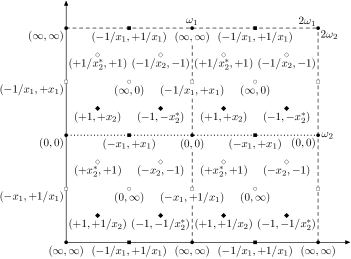
$$x_{1}=i\sqrt{\frac{\sqrt{1+16g^{2}}-1}{\sqrt{1+16g^{2}}+1}}\,,\qquad x_{2}=\frac{\sqrt{1+4ig}-1}{\sqrt{1+4ig}+1}\,$$

Figure 14: Some special points $(x^{+},x^{-})$ in the rapidity plane.

We have already discussed shifts by the real half-period which act trivially. A shift by an imaginary half-period acts as

$$x^{\pm}(z+\omega_{2})=1/x^{\pm}(z)\,,\qquad u(z+\omega_{2})=u(z)\,,\qquad C(z+\omega_{2})=-C(z).$$ (A.10)

This map essentially interchanges the representation with its conjugate. It is called the antipode map and it plays a central role for crossing symmetry, see Sec. 3.7. In addition to these, there are further interesting discrete transformations of the rapidity plane. An extensive list is given in Tab. 3. The transformations of the maps can be verified using the addition formulas of elliptic functions $\mathop{\operator@font sn}\nolimits,\mathop{\operator@font cn}\nolimits,\mathop{\operator@font dn}\nolimits$. Of particular interest may be the map $z\mapsto-z$. This map inverts the momentum but leaves the energy invariant. It thus represents parity inversion.

Points invariant under some of the transformations are shown in Fig. 14. They are all of the form $z={\textstyle\frac{1}{4}}m_{1}\omega_{1}+{\textstyle\frac{1}{4}}m_{2}\omega_{2}$ with $m_{1}+m_{2}$ even. At these points the parameters $x^{+},x^{-}$ take special values: The values $0,\infty$ are invariant under taking the negative and $\pm 1$ are invariant under inversion. The remaining points are such that the product or quotient of $x^{\pm}$ is $-1$.

References

• [1] J. M. Maldacena, “The large N limit of superconformal field theories and supergravity”, Adv. Theor. Math. Phys. 2, 231 (1998), hep-th/9711200.
• [2] S. S. Gubser, I. R. Klebanov and A. M. Polyakov, “Gauge theory correlators from non-critical string theory”, Phys. Lett. B428, 105 (1998), hep-th/9802109.
• [3] E. Witten, “Anti-de Sitter space and holography”, Adv. Theor. Math. Phys. 2, 253 (1998), hep-th/9802150.
• [4] G. ’t Hooft, “A Planar Diagram Theory for Strong Interactions”, Nucl. Phys. B72, 461 (1974).
• [5] O. Aharony, S. S. Gubser, J. M. Maldacena, H. Ooguri and Y. Oz, “Large N field theories, string theory and gravity”, Phys. Rept. 323, 183 (2000), hep-th/9905111.
• [6] E. D’Hoker and D. Z. Freedman, “Supersymmetric gauge theories and the AdS/CFT correspondence”, hep-th/0201253, in: “Strings, Branes And Extra Dimensions”, ed.: S. S. Gubser and J. D. Lykken, World Scientific (2004), Singapore.
• [7] J. A. Minahan and K. Zarembo, “The Bethe-ansatz for $\mathcal{N}=\mathord{}$4 super Yang-Mills”, JHEP 0303, 013 (2003), hep-th/0212208.
• [8] N. Beisert, C. Kristjansen and M. Staudacher, “The Dilatation Operator of $\mathcal{N}=\mathord{}$4 Conformal Super Yang-Mills Theory”, Nucl. Phys. B664, 131 (2003), hep-th/0303060.
• [9] N. Beisert and M. Staudacher, “The $\mathcal{N}=\mathord{}$4 SYM Integrable Super Spin Chain”, Nucl. Phys. B670, 439 (2003), hep-th/0307042.
• [10] L. N. Lipatov, “Evolution equations in QCD”, in: “Perspectives in Hadronic Physics”, ed.: S. Boffi, C. Ciofi Degli Atti and M. Giannini, World Scientific (1998), Singapore.
• [11] V. M. Braun, S. E. Derkachov and A. N. Manashov, “Integrability of three-particle evolution equations in QCD”, Phys. Rev. Lett. 81, 2020 (1998), hep-ph/9805225.
• [12] A. V. Belitsky, “Fine structure of spectrum of twist-three operators in QCD”, Phys. Lett. B453, 59 (1999), hep-ph/9902361.
• [13] G. Mandal, N. V. Suryanarayana and S. R. Wadia, “Aspects of semiclassical strings in $AdS_{5}$, Phys. Lett. B543, 81 (2002), hep-th/0206103.
• [14] I. Bena, J. Polchinski and R. Roiban, “Hidden symmetries of the $AdS_{5}\times S^{5}$ superstring”, Phys. Rev. D69, 046002 (2004), hep-th/0305116.
• [15] G. Arutyunov, S. Frolov and M. Staudacher, “Bethe ansatz for quantum strings”, JHEP 0410, 016 (2004), hep-th/0406256.
• [16] N. Beisert and M. Staudacher, “Long-Range PSU(2,2$/$4) Bethe Ansaetze for Gauge Theory and Strings”, Nucl. Phys. B727, 1 (2005), hep-th/0504190.
• [17] N. Beisert, “The Dilatation Operator of $\mathcal{N}=\mathord{}$4 Super Yang-Mills Theory and Integrability”, Phys. Rept. 405, 1 (2004), hep-th/0407277.
• [18] K. Zarembo, “Semiclassical Bethe ansatz and AdS/CFT”, Comptes Rendus Physique 5, 1081 (2004), hep-th/0411191.
• [19] J. Plefka, “Spinning strings and integrable spin chains in the AdS/CFT correspondence”, Living. Rev. Relativity 8, 9 (2005), hep-th/0507136.
• [20] A. V. Belitsky, V. M. Braun, A. S. Gorsky and G. P. Korchemsky, “Integrability in QCD and beyond”, Int. J. Mod. Phys. A19, 4715 (2004), hep-th/0407232.
• [21] R. R. Metsaev and A. A. Tseytlin, “Type IIB superstring action in $AdS_{5}\times S^{5}$ background”, Nucl. Phys. B533, 109 (1998), hep-th/9805028.
• [22] N. Y. Reshetikhin and P. B. Wiegmann, “Towards the classification of completely integrable quantum field theories”, Phys. Lett. B189, 125 (1987).
• [23] H. Bethe, “Zur Theorie der Metalle I. Eigenwerte und Eigenfunktionen der linearen Atomkette”, Z. Phys. 71, 205 (1931).
• [24] B. Sutherland, “A brief history of the quantum soliton with new results on the quantization of the Toda lattice”, Rocky Mtn. J. Math. 8, 413 (1978).
• [25] M. Staudacher, “The factorized S-matrix of CFT/AdS”, JHEP 0505, 054 (2005), hep-th/0412188.
• [26] D. Berenstein, J. M. Maldacena and H. Nastase, “Strings in flat space and pp waves from $\mathcal{N}=\mathord{}$4 Super Yang Mills”, JHEP 0204, 013 (2002), hep-th/0202021.
• [27] N. Beisert, “The SU(2$/$2) Dynamic S-Matrix”, hep-th/0511082.
• [28] G. Arutyunov, S. Frolov, J. Plefka and M. Zamaklar, “The Off-shell Symmetry Algebra of the Light-cone $AdS_{5}\times S^{5}$ Superstring”, hep-th/0609157.
• [29] N. Y. Reshetikhin, “A method of functional equations in the theory of exactly solvable quantum system”, Lett. Math. Phys. 7, 205 (1983).
• [30] R. A. Janik, “The $AdS_{5}\times S^{5}$ superstring worldsheet S-matrix and crossing symmetry”, Phys. Rev. D73, 086006 (2006), hep-th/0603038.
• [31] N. Beisert, “On the scattering phase for $AdS_{5}\times S^{5}$ strings”, hep-th/0606214.
• [32] N. Beisert, R. Hernández and E. López, “A Crossing-Symmetric Phase for $AdS_{5}\times S^{5}$ Strings”, JHEP 0611, 070 (2006), hep-th/0609044.
• [33] J. Hubbard, “Electron Correlations in Narrow Energy Bands”, Proc. R. Soc. London A276, 238 (1963).
• [34] E. H. Lieb and F. Y. Wu, “Absence of Mott transition in an exact solution of the short-range, one-band model in one dimension”, Phys. Rev. Lett. 20, 1445 (1968).
• [35] F. H. L. Essler, H. Frahm, F. Göhmann, A. Klümper and V. E. Korepin, “The one-dimensional Hubbard model”, Cambridge University Press (2005), Cambridge, UK, 690p.
• [36] B. S. Shastry, “Exact Integrability of the One-Dimensional Hubbard Model”, Phys. Rev. Lett. 56, 2453 (1986).
• [37] A. Rej, D. Serban and M. Staudacher, “Planar $\mathcal{N}=\mathord{}$4 Gauge Theory and the Hubbard Model”, JHEP 0603, 018 (2006), hep-th/0512077.
• [38] K. Iohara and Y. Koga, “Central extensions of Lie superalgebras”, Comment. Math. Helv. 76, 110 (2001).
• [39] A. H. Kamupingene, H. A. Ky and T. D. Palev, “Finite-Dimensional representations of the Lie superalgebra gl(2$/$2) in a $gl(2)\oplus gl(2)$ basis. I. Typical representations”, J. Math. Phys. 30, 553 (1989).
• [40] T. D. Palev and N. I. Soilova, “Finite-Dimensional representations of the Lie superalgebra gl(2$/$2) in a $gl(2)\oplus gl(2)$ basis. II. Nontypical representations”, J. Math. Phys. 31, 953 (1990).
• [41] Y.-Z. Zhang and M. D. Gould, “A Unified and Complete Construction of All Finite Dimensional Irreducible Representations of gl(2$/$2)”, J. Math. Phys. 46, 013505 (2005), math.qa/0405043.
• [42] G. Götz, T. Quella and V. Schomerus, “Tensor products of psl(2$/$2) representations”, hep-th/0506072.
• [43] G. Götz, T. Quella and V. Schomerus, “The WZNW model on PSU(1,1$/$2)”, hep-th/0610070.
• [44] A. B. Balantekin and I. Bars, “Dimension and character formulas for Lie supergroups”, J. Math. Phys. 22, 1149 (1981).
• [45] N. Beisert, “The SU(2$/$3) Dynamic Spin Chain”, Nucl. Phys. B682, 487 (2004), hep-th/0310252.
• [46] A. B. Zamolodchikov and A. B. Zamolodchikov, “Factorized S-matrices in two dimensions as the exact solutions of certain relativistic quantum field models”, Annals Phys. 120, 253 (1979).
• [47] D. M. Hofman and J. M. Maldacena, “Giant magnons”, J. Phys. A39, 13095 (2006), hep-th/0604135.
• [48] H. Lin, O. Lunin and J. M. Maldacena, “Bubbling AdS space and 1/2 BPS geometries”, JHEP 0410, 025 (2004), hep-th/0409174.
• [49] C. Gomez and R. Hernández, “The magnon kinematics of the AdS/CFT correspondence”, JHEP 0611, 021 (2006), hep-th/0608029.
• [50] J. Plefka, F. Spill and A. Torrielli, “On the Hopf algebra structure of the AdS/CFT S-matrix”, Phys. Rev. D74, 066008 (2006), hep-th/0608038.
• [51] N. Beisert and A. A. Tseytlin, “On Quantum Corrections to Spinning Strings and Bethe Equations”, Phys. Lett. B629, 102 (2005), hep-th/0509084.
• [52] R. Hernández and E. López, “Quantum corrections to the string Bethe ansatz”, JHEP 0607, 004 (2006), hep-th/0603204.
• [53] L. Freyhult and C. Kristjansen, “A universality test of the quantum string Bethe ansatz”, Phys. Lett. B638, 258 (2006), hep-th/0604069.
• [54] G. Arutyunov and S. Frolov, “On $AdS_{5}\times S^{5}$ string S-matrix”, Phys. Lett. B639, 378 (2006), hep-th/0604043.
• [55] N. Dorey, “Magnon bound states and the AdS/CFT correspondence”, J. Phys. A39, 13119 (2006), hep-th/0604175.
• [56] N. Beisert and R. Roiban, “Beauty and the Twist: The Bethe Ansatz for Twisted $\mathcal{N}=\mathord{}$4 SYM”, JHEP 0508, 039 (2005), hep-th/0505187.
• [57] Z. Maassarani, “Uq(osp)(2,2) lattice models”, J. Phys. A28, 1305 (1995), hep-th/9407032.
• [58] A. J. Bracken, M. D. Gould, J. R. Links and Y.-Z. Zhang, “A New Supersymmetric and Exactly Solvable Model of Correlated Electrons”, Phys. Rev. Lett. 74, 2768 (1995), cond-mat/9410026.
• [59] M. P. Pfannmüller and H. Frahm, “Algebraic Bethe Ansatz for gl(2,1) Invariant 36-Vertex Models”, Nucl. Phys. B479, 575 (1996), cond-mat/9604082.
• [60] N. Beisert, “An SU(1$/$1)-Invariant S-Matrix with Dynamic Representations”, Bulg. J. Phys. 33S1, 371 (2006), hep-th/0511013.
• [61] F. Woynarowich, “Low-energy excited states in a Hubbard chain with on-site attraction”, J. Phys. C16, 6593 (1983).
• [62] P.-A. Bares, J. M. P. Carmelo, J. Ferrer and P. Horsch, “Charge-spin recombination in the one-dimensional supersymmetric t-J model”, Phys. Rev. B46, 14624 (1992).
• [63] F. H. L. Essler and V. E. Korepin, “A New solution of the supersymmetric T-J model by means of the quantum inverse scattering method”, hep-th/9207007.
• [64] N. Beisert, V. A. Kazakov, K. Sakai and K. Zarembo, “Complete Spectrum of Long Operators in $\mathcal{N}=\mathord{}$4 SYM at One Loop”, JHEP 0507, 030 (2005), hep-th/0503200.
• [65] O. J. Heilmann and E. H. Lieb, “Violation of the Noncrossing Rule: The Hubbard Hamiltonian for Benzene”, New York Academy of Sciences (1971), New York, USA.
• [66] C. N. Yang, $\eta$ Pairing and Off-Diagonal Long-Range Order in a Hubbard Model”, Phys. Rev. Lett. 63, 2144 (1989).
• [67] C. N. Yang and S. C. Zhang, $SO(4)$ Symmetry in a Hubbard Model”, Mod. Phys. Lett. B4, 759 (1990).
• [68] P. B. Ramos and M. J. Martins, “Algebraic Bethe ansatz approach for the one-dimensional Hubbard model”, J. Phys. A30, L195 (1997), hep-th/9605141.
• [69] F. Göhmann, unpublished.
• [70] H.-Q. Zhou, “Quantum integrability for the one-dimensional Hubbard open chain”, Phys. Rev. B54, 41 (1996).
• [71] M. Shiroishi and M. Wadati, “Integrable Boundary Conditions for the One-Dimensional Hubbard Model”, J. Phys. Soc. Jap. 66, 2288 (1997), cond-mat/9708011.
• [72] F. H. L. Essler, V. E. Korepin and K. Schoutens, “New exactly solvable model of strongly correlated electrons motivated by high T(c) superconductivity”, Phys. Rev. Lett. 68, 2960 (1992), cond-mat/9209002.
• [73] F. C. Alcaraz and R. Z. Bariev, “Interpolation between Hubbard and supersymmetric t-J models: two-parameter integrable models of correlated electrons”, J. Phys. A32, L483 (1999), cond-mat/9908265.
• [74] X.-W. Guan, A. Foerster, L. J., H.-Q. Zhou, A. Prestes Tonel and R. H. McKenzie, “Integrable variant of the one-dimensional Hubbard model”, J. Math. Phys. 43, 3445 (2002), cond-mat/0103059.
• [75] M. J. Martins and P. B. Ramos, “The Quantum Inverse Scattering Method for Hubbard-like Models”, Nucl. Phys. B522, 413 (1998), solv-int/9712014.
• [76] F. Göhmann, “Algebraic Bethe ansatz for the gl(1$/$2) generalized model and Lieb-Wu equations”, Nucl. Phys. B620, 501 (2002), cond-mat/0108486.
• [77] B. S. Shastry, “Decorated star-triangle relations and exact integrability of the one-dimensional Hubbard model”, J. Stat. Phys. 50, 57 (1988).
• [78] R. Yue and T. Deguchi, “Analytic Bethe Ansatz for 1-D Hubbard model and twisted coupled XY model”, J. Phys. A30, 849 (1997), cond-mat/9606039.
• [79] I. Krichever, O. Lipan, P. Wiegmann and A. Zabrodin, “Quantum integrable models and discrete classical Hirota equations”, Commun. Math. Phys. 188, 267 (1997), hep-th/9604080.
• [80] P. P. Kulish and N. Y. Reshetikhin, “On GL3-invariant solutions of the Yang-Baxter equation and associated quantum systems”, J. Math. Sci. 34, 1948 (1986).
• [81] M. Jimbo, T. Miwa and M. Okado, “An $A^{(1)}_{n-1}$ family of solvable lattice models”, Mod. Phys. Lett. B1, 73 (1987).
• [82] N. Beisert, V. Kazakov, K. Sakai and K. Zarembo, “The Algebraic Curve of Classical Superstrings on $AdS_{5}\times S^{5}$, Commun. Math. Phys. 263, 659 (2006), hep-th/0502226.
• [83] N. Dorey and B. Vicedo, “On the dynamics of finite-gap solutions in classical string theory”, JHEP 0607, 014 (2006), hep-th/0601194.
• [84] V. I. Inozemtsev, “Integrable Heisenberg-van Vleck chains with variable range exchange”, Phys. Part. Nucl. 34, 166 (2003), hep-th/0201001.
• [85] D. Serban and M. Staudacher, “Planar $\mathcal{N}=\mathord{}$4 gauge theory and the Inozemtsev long range spin chain”, JHEP 0406, 001 (2004), hep-th/0401057.
• [86] S. Schäfer-Nameki, M. Zamaklar and K. Zarembo, “Quantum corrections to spinning strings in $AdS_{5}\times S^{5}$ and Bethe ansatz: A comparative study”, JHEP 0509, 051 (2005), hep-th/0507189.
• [87] S. Schäfer-Nameki and M. Zamaklar, “Stringy sums and corrections to the quantum string Bethe ansatz”, JHEP 0510, 044 (2005), hep-th/0509096.
• [88] S. Schäfer-Nameki, “Exact expressions for quantum corrections to spinning strings”, Phys. Lett. B639, 571 (2006), hep-th/0602214.
• [89] J. Ambjørn, R. A. Janik and C. Kristjansen, “Wrapping interactions and a new source of corrections to the spin-chain / string duality”, Nucl. Phys. B736, 288 (2006), hep-th/0510171.
• [90] N. Mann and J. Polchinski, “Finite density states in integrable conformal field theories”, hep-th/0408162, in: “From Fields to Stings: Circumnavigating Theoretical Physics”, ed.: M. Shifman, A. Vainshtein and J. Wheater, World Scientific (2005), Singapore.
• [91] N. Mann and J. Polchinski, “Bethe ansatz for a quantum supercoset sigma model”, Phys. Rev. D72, 086002 (2005), hep-th/0508232.
• [92] N. Gromov, V. Kazakov, K. Sakai and P. Vieira, “Strings as multi-particle states of quantum sigma-models”, hep-th/0603043.
• [93] J. Teschner, “The Sinh-Gordon Model — A Warm-Up for Noncompact Nonlinear Sigma Models?”, Talk at Workshop on Integrability in Gauge and String Theory, AEI, Potsdam, Germany, July 24-28, 2006, http://int06.aei.mpg.de/presentations/teschner.pdf.
• [94] A. G. Bytsko and J. Teschner, “Quantization of models with non-compact quantum group symmetry: Modular XXZ magnet and lattice sinh-Gordon model”, J. Phys. A39, 12927 (2006), hep-th/0602093.