Freely decaying turbulence and Bose-Einstein condensation in Gross-Pitaevski model

Abstract

We study turbulence and Bose-Einstein condensation (BEC) within the two-dimensional Gross-Pitaevski (GP) model. In the present work, we compute decaying GP turbulence in order to establish whether BEC can occur without forcing and if there is an intensity threshold for this process. We use the wavenumber-frequency plots which allow us to clearly separate the condensate and the wave components and,therefore, to conclude if BEC is present. We observe that BEC in such a system happens even for very weakly nonlinear initial conditions without any visible threshold. BEC arises via a growing phase coherence due to anihilation of phase defects/vortices. We study this process by tracking of propagating vortex pairs. The pairs loose momentum by scattering the background sound, which results in gradual decrease of the distance between the vortices. Occasionally, vortex pairs collide with a third vortex thereby emitting sound, which can lead to more sudden shrinking of the pairs. After the vortex anihilation the pulse propagates further as a dark soliton, and it eventually bursts creating a shock.

1 Background and motivation

For dilute gases with large energy occupation numbers the Bose-Einstein condensation (BEC) [3, 4, 5] can be described by the Gross-Pitaevsky (GP) equation [1, 2]:

$$i\Psi_{t}+\Delta\Psi-|\Psi|^{2}\Psi=0,$$ (1)

where $\Psi$ is the condensate “wave function”. GP equation also describes light behavior in media with Kerr nonlinearities.

Many interesting features were found in GP turbulence in both the nonlinear optics and BEC contexts [6, 7, 8, 9, 12, 11]. Initial fields, if weak, behave as wave turbulence (WT) where the main nonlinear process is a four-wave resonant interaction described by a four-wave kinetic equation [7]. This closure was used in [6, 8, 9] to describe the initial stage of BEC. It was also theoretically predicted that the four-wave WT closure will eventually fail due to emergence of a coherent condensate state which is uniform in space [9]. At this stage the nonlinear dynamics can be represented as interactions of small perturbations about the condensate state. Once again, one can use WT to describe such a system, but now the leading process will be a three-wave interaction of acoustic-like waves on the condensate background [9]. Coupling of such acoustic turbulence to the condensate was considered in [15] which allowed to derived the asymptotic law of the condensate growth.

In [10], the stage of transition from the four-wave to the three-wave WT regimes, which itself is a strongly nonlinear process involving a gas of strongly nonlinear vortices, was studied. These vortices anihilate and their number reduces to zero in a finite time, marking a finite-time growth of the correlation length of the phase of $\Psi$ to infinity. This is similar to the Kibble-Zurek mechanism of the early Universe phase transitions which has been introduced originally in cosmology [16, 17]. It has been established that the vortex anihilation process is aided by the presence of sound and it becomes incomplete if sound is dissipated. Fourier transforms in both space and time were analysed using the wavenumber-frequency plots which, in case of weak wave turbulence, are narrowly concentrated around the linear dispersion relation $\omega=\omega_{k}$. At the initial stage, narrow $(k,\omega)$-distributions around $\omega=\omega_{k}=k^{2}$, were seen whereas at late evolution stages we saw two narrow components: a condensate at horizontal line $\omega=\langle\rho\rangle=\langle|\Psi|^{2}\rangle$ and an acoustic component in proximity of the Bogolyubov curve $\Omega_{k}=\langle\rho\rangle+\sqrt{k^{4}+2\langle\rho\rangle k^{2}}$.

In [10], the system was continuously forced at either large or small scales because this is a classical WT setting. WT predictions were confirmed for the energy spectra of GP turbulence. However, it remained unclear if presence of forcing is essential for complete BEC process, and whether there is any intensity threshold for this process in the absence of forcing. This questions are nontrivial because, in principle, even a weakly forced system could behave very differently from the forced one due to an infinite supply of particles over long time.

In the present paper we will examine these questions via numerical simulations of the 2D GP model without forcing. In addition, we will carefully examine and describe the essential stages of the typical route to the vortex anihilation leading to BEC. In many ways our work is closely related with numerical studies of decaying 3D GP turbulence of Ref. [12], where transition from the 4-wave WT regime to condensation and superfluidity was studied by visualising emergence and decay of a superfluid vortex tangle. However, our work addresses additional issues which were not discussed in the previous papers, particularly emergence and dispersive properties of the 3-wave acoustic turbulence, crucial role of sound for the vortex decay process, separating the wave and the condensate components using novel numerical diagnostics based on $(k,\omega)$-distributions.

Below, we will only describe our numerical setup and results. For a summary of WT theory and its predictions in the GP context we reffer to our previous paper [10].

2 Setup for numerical experiments

In this paper we consider a setup corresponding to homogeneous turbulence and, therefore, we ignore finite-size effects due to magnetic trapping in BEC or to the finite beam radii in optical experiments. For numerical simulations, we have used a standard pseudo-spectral method [18] for the 2D equation (1): the nonlinear term is computed in physical space while the linear part is solved exactly in Fourier space. The integration in time is performed using a second-order Runge-Kutta method. The number of grid points in physical space was set to $N\times N$ with $N=256$. Resolution in Fourier space was $\Delta k=2\pi/N$. Sink at high wave numbers was provided by adding to the right hand side of equation (1) the hyper-viscosity term $\nu(-\nabla^{2})^{n}\psi$. Values of $\nu$ and $n$ were selected in order to localized as much as possible dissipation to high wave numbers but avoiding at the same time the bottleneck effect, - a numerical artifact of spectrum pileup at the smallest scales [13]. Note that importance of introducing the small-scale dissipation to eliminate the bottleneck effect has long been realised in numerical simulations of classical Navier-Stokes fluids, and it was also recently realised in the context of GP turbulence in [14]. We have found, after a number of trials, that $\nu=2\times 10^{-6}$ and $n=8$ were good choices for our purposes. Time step for integration was depended on the initial conditions. For strong nonlinearity smaller time step were required. Numerical simulations were performed on a PowerPC G5, 2.7 Ghz. Initial conditions were provided by the following:

$$\psi(k_{x},k_{y},t=0)=\frac{\alpha}{\sqrt{\pi^{1/2}\sigma}}e^{-\frac{(k-k_{0})^{2}}{2\sigma^{2}}}e^{i\phi}$$ (2)

where $k=\sqrt{k_{x}^{2}+k_{y}^{2}}$. $\alpha$ is a real number which was varied in order to change the nonlinearity of the initial condition for different simulations. $\phi=\phi(k_{x},k_{y})$ are uniformly distributed random numbers in the interval $[0,2\pi]$. The simulations that will be presented here have been obtained with $k_{0}$= 35 $\Delta k$ and $\sigma=5\Delta k$. The nonlinearity of the initial condition was measured as $\varepsilon$=$k_{0}\alpha$. We have performed simulations ranging from $\varepsilon_{min}=0.018$ to $\varepsilon_{max}=1.3$, so we have spanned almost 2 decades of nonlinear parameter in the initial conditions.

3 Numerical results

3.1 Evolving spectra

We start by examining the most popular turbulence object, the spectrum,

$$n_{k}=\langle|\Psi_{k}|^{2}\rangle.$$

Since we study the setup corresponding to BEC, we start with a spectrum concentrated at high wavenumbers leaving a range of smaller wavenumbers initially empty so that it could be filled during the evolution. In figures 1 and 2 we show the spectra at different times for the strongest and the weakest nonlinear initial condition we have analyzed.

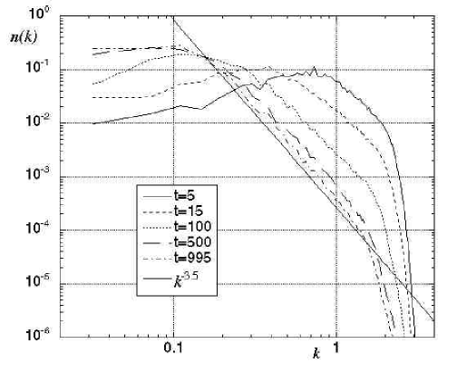
Figure 1: Spectra at different times for the initial condition characterized by $\varepsilon=1.3$

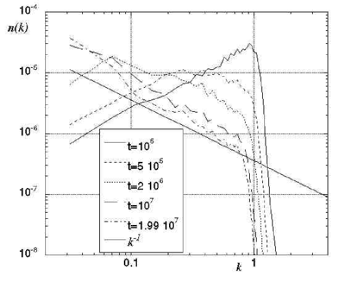
Figure 2: Spectra at different times for the initial condition characterized by $\varepsilon=0.018$

At early stages, for both small and large initial intensities, we see propagation of the spectrum toward lower wavenumbers. However, we do not observe formation of a scaling range corresponding to the wave energy equipartition $n_{k}\sim 1/\omega_{k}=1/k^{2}$ (i.e. energy density $\omega_{k}n_{k}$ is constant in the 2D $k$-space) as it was the case in the simulations with continuous forcing [10].

At later stages, no matter how small the initial intensity is, the low-k front reaches the smallest wavenumber and we observe steepening reaching slope $\sim-3.5$ for large initial intensities (figure 1) and $\sim-1$ for the weakest initial data (figure 2). This corresponds to WT breakdown and onset of BEC. However, the information contained in spectrum $n_{k}$ is very incomplete as it does not allow to distinguish between the coherent condensate and random waves that may both occupy the same wavenumber range. Thus, we turn to study the direct measures of condensation such as the correlation length and the wavenumber-frequency plots.

3.2 Explosive growth of correlation length

By definition, condensate is a coherent structure whose correlation length is of the same order as the bounding box. We define the correlation length directly based on the auto-correlation function of field $\Psi$,

$$C_{\psi}(r)=\langle{\cal R}\Psi({\bf x})\,{\cal R}\Psi({\bf x+r})\rangle/\langle{\cal R}\Psi({\bf x})^{2}\rangle,$$ (3)

where ${\cal R}\Psi$ denotes the real part of $\Psi$ (result based on the imaginary part would be equivalent). Correlation length $\lambda$ can be defined as

$$\lambda^{2}=\int_{0}^{r_{0}}C_{\psi}(r)\,d{\bf r},$$ (4)

where $r_{0}$ is the first zero of $C_{\psi}(r)$. Note that initially $C_{\psi}(r)$ can strongly oscillate, which is a signature of weakly nonlinear waves. However, only one oscillation (i.e. within the first zero crossing) is relevant to the condensate, which explains our definition of $\lambda$. Figure 3 shows evolution of $1/\lambda^{2}$ which, as we see that $\lambda$ always reaches the box size wich is a signature of BEC.

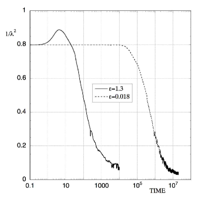
Figure 3: Evolution in time of the correlation length for different nonlinearity.

3.3 Wavenumber-Frequency plots

As we discussed above, the spectra cannot distinguish between random waves and coherent structures especially when they are present simultaneously and overlap in the $k$-space. Besides, the spectra do not tell us if the wave component is weakly or strongly nonlinear. To resolve these ambiguities, following [10], let us perform an additional Fourier transform over a window of time and examine the resulting $(k,\omega)$-plots of space-time Fourier coefficients.

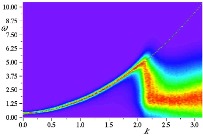
Figure 4: ($k,\omega)$ plot for the initial stage for the case of $\varepsilon=0.4$. Solid curve shows the Bogolyubov dispersion relation.

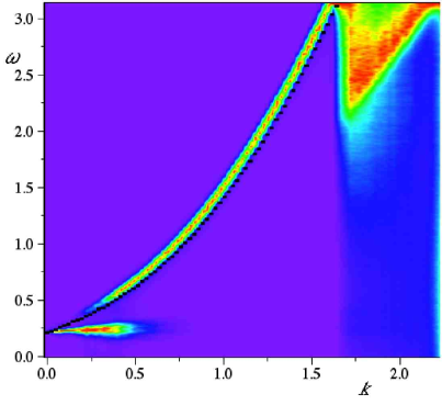
Figure 5: ($k,\omega)$ plot for the late stage for the case of $\varepsilon=0.4$. Solid curve shows the Bogolyubov dispersion relation.

Figure 4 corresponds to an early time of the system with relatively weak initial intensity ($\varepsilon=0.4$). We see that the distribution is narrowly concentrated near $\omega=k^{2}$ which indicates that these waves are weakly nonlinear. The weak nonlinear effects manifestate themselves in a small up-shift and broadening of the $(k,\omega)$-distribution with respect to the $\omega=k^{2}$ curve. For sufficiently small initial intensities, these early stages of evolution are characterised by weak 4-wave turbulence. The breakdown of the $\omega=k^{2}$ curve at high $k$’s occurs due to the the numerical dissipation in the region close to the maximal wavenumber (this component is weak but clearly visible because the color map is normalised to the maximal value of the spectrum at each fixed $k$).

Figure 5 shows a late-time plot for the same run (i.e. $\varepsilon=0.4$). The late-stage $(k,\omega)$-plots for the most nonlinear intensities are in shown in figure 6. We see that in both cases we now see two clearly separated components quite narrowly concentrated around the following curves:

• (A) A horizontal line with $\omega\approx\langle\rho\rangle$,

• (B) The upper curve which follows the Bogolyubov curve $\omega=\Omega_{k}=\langle\rho\rangle+\sqrt{k^{4}+2\langle\rho\rangle k^{2}}$.

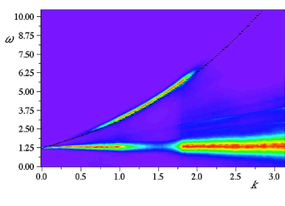
Figure 6: ($\omega-k)$ plot for the latest stages for the most nonlinear case, $\varepsilon=1.3$. Solid curve shows the Bogolyubov dispersion relation.

Component (A) corresponds to BEC. Its coherency can be seen in the fact that the frequency of different wavenumbers is the same. Note that usually BEC is depicted as a component with the lowest possible wavenumber in the system, whereas in our case we see a spread over, although small, but finite range of wavenumbers. This wavenumber spread is caused by few remaining deffects/vortices.

Curve (B) corresponds the Bogolyubov sound-like waves. We see that the the $(k,\omega)$-distribution is quite narrow and close to the Bogolyubov dispersion curve, which indicates that these waves are weakly nonlinear. However, now these weakly nonlinear waves travel on a strongly nonlinear BEC background. This is a three-wave acoustic weak turbulence regime [9, 15, 10].

3.4 Separating the condensate and the wave components

Using the Wavenumber-Frequency plots we can separate BEC and the wave component and plot their spectra separately. In figure 7 we show the spectrum for the case of $\varepsilon=1.3$ at late time for the condensate and the rest of the wave field. These spectra have been obtained by integrating the $(\omega-k)$ from 0 to a threshold $\omega_{c}$ (this corresponds to condensate) and from $\omega_{c}$ to the maximum value of $\omega$ considered. In the present case, in order to separate the condensate, $\omega_{c}$ was set to 1.5 (see figure 6).

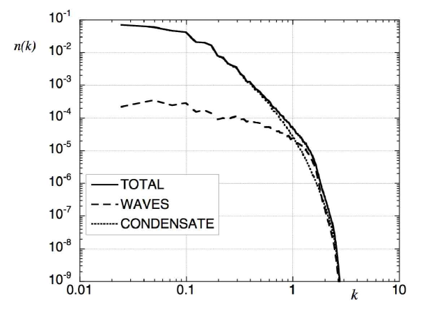
Figure 7: Total wave spectrum (solid line), condensate wave spectrum (dotted line) and background wave spectrum (dotted line)

As is clear from the the figure, most of the energy is concentrated in the condensate.

3.5 Typical events leading to vortex anihilation

Vortices ar phase deffects of $\Psi$ and, therefore, the correlation length growth is intimately connected with the decrease of the total number of vortices. As argued in [10] that $N_{vortices}\sim 1/\lambda^{2}$. To give an illustration of the anihilation process we show in figure 8 two snapshots of $|\Psi(x,y,t)|$ at different times. The vortices are seen as blue spots in these snapshots and we see a considerable decrease of their number at the later time (on the right).

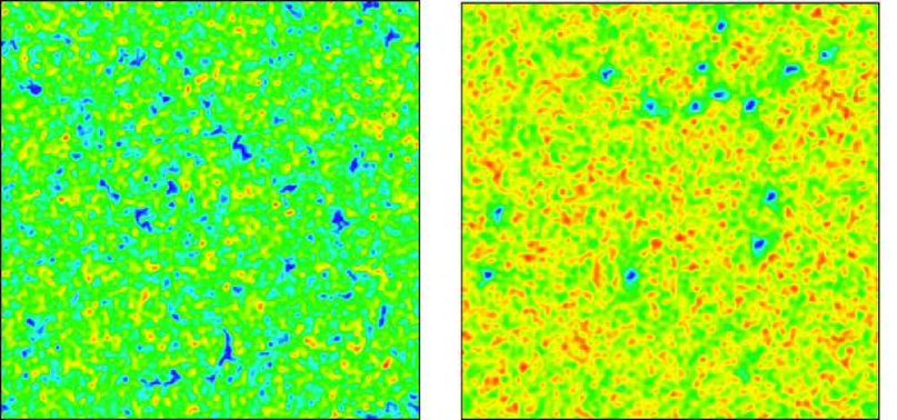
Figure 8: $|\Psi(x,y,t))|$ at two different instants of time

It was shown in [10] that Bogolyubov sound is an essential mediator in the vortex anihilation process, and that introducing a sound absorption can lead to frustration and incompleteness of the BEC process.

Let us now examine in detail the typical sequence of events leading to the vortex annihilation by tracking vortex pairs that are destined to anihilate. The vortex pair motion is best seen in a computer generated movie which is available upon request from the authors. In Figures 9, 10 and 11 we show a representative sequence of frames from this movie.

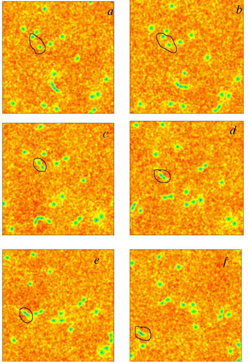
Figure 9:

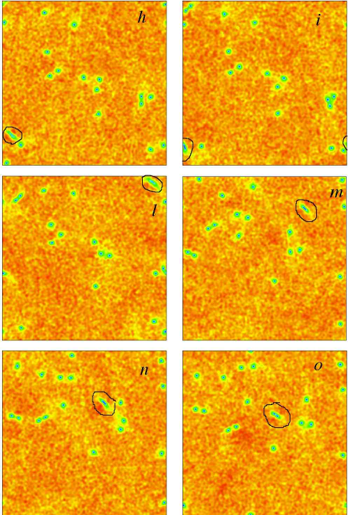
Figure 10:

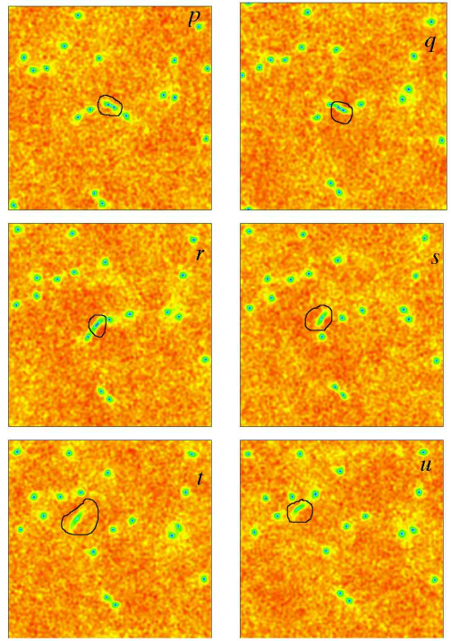
Figure 11:

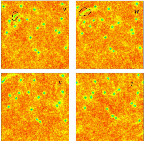
Figure 12:

We can see that the vortex pair forms in frames a to c so that the distance between the vortices in the pair is considerably less than distance to the other vortices. Such a pair propagates like a vortex dipole in fluid, as seen in frames c to f. During this propagation, the vortex pair scatters the ambient sound waves thereby transferring its momentum to the acoustic field. This momentum loss make vortices get closer to each other and, therefore, move faster as a pair. This process can be interpreted as a “friction” between the vortices and a “normal component” (phonons). It is easy to show that such process leads to the change of distance $d(t)$ between the vortices like

$$d(t)=\alpha\sqrt{t^{A}-t},$$ (5)

where coefficient $\alpha$ is proportional to the energy density of sound and $t^{A}$ is the anihilation time.

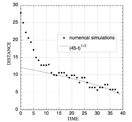
Figure 13: Distance between a pair vortices as a function of time for the vortex pair and the time range of Figure 9.

Figure 13 shows evolution of the inter-vortex distance $d(t)$, calculated for the vortex pair and the time range of Figure 9. We see that for the time range when the vortex pair is more or less isolated from the other vortices, $11<t<40$, the inter-vortex distance shrinks in qualitative agreement with law (5). However, immediately after that, in frame h in Figure 10, the vortex pair collide with a third vortex and suddenly shrink and anihilate. Further on the movie we see that the vortex pair momentum was not completely lost and it keep propagating a Jones-Roberts dark soliton [19]. In between of frames h and o the soliton “cannot make up his mind” oscillating between the state with and without vortices near the vortex anihilation threshold, until frame p where it re-emerges as a vortex pair. It collides with yet another vortex and changes its propagation direction to 90 degree in between of frames q and r, it annihilates again in frame s, propagates as a dark soliton until frame v. Eventually, this soliton is weakened due to further sound generation and scattering and it becomes too weak to maintain its stability and integrity. At this point it bursts thereby generating a shock wave as seen in frames v to y.

Summarizing, we can identify the following important events on the route to vortex anihilation:

• Gradual shrinking of the inter-vortex distance due to the sound scattering when the vortex pair is sufficiently isolated from the rest of the vortices,

• Sudden shrinking events due to collisions with a third vortex and resulting sound generation (similar three-vortex event was described in [20]),

• Post-anihilation propagation of dark solitons,

• Occasional recovery of vortex pairs in dark solitons which are close to the critical amplitude,

• Weakening and loss of stability of the dark solitons resulting in a shock wave.

4 Conclusions

We have computed decaying GP turbulence in a 2D periodic box with initial spectrum occupying the small-scale range. We observed that BEC at large scales arises for any initial intensity without a visible threshold, even for very weakly nonlinear initial conditions. BEC was detected by analysing the spectra and the correlation length and, most clearly, by analysing the $(k,\omega)$ plots. On these plots BEC and Bogolyubov waves are seen as two clearly distinct components: (i) BEC coherently oscillating at nearly constant frequency and (ii) weakly nonlinear waves closely following the Bogolyubov dispersion. By separating BEC and the waves we observed that most of the energy at late times is residing in the BEC component at most of the important scales except for the smallest ones.

We also analysed the typical events on the path to vortex anihilation, - an essential mechanism of BEC.

Acknowledgments
Al Osborne is acknowledged for discussions in the early stages of the work.

References

- [1] E.P. Gross, Structure of a quantized vortex in boson systems, Nuovo Cimento, 20, 454, (1961).
- [2] L.P. Pitaevsky, Vortex lines in an imperfect Bose gas, Sov. Phys. JETP, 13, 451 (1961).
- [3] M. H. Anderson, J.R. Ensher, M.R. Matthews, C.E. Wieman, E.A. Cornell, Observation of Bose-Einstein Condensation in a Dilute Atomic Vapor, Science 269, 198 (1995).
- [4] C. C. Bradley, C. A. Sackett, J. J. Tollett, and R. G. Hulet, Evidence of Bose-Einstein Condensation in an Atomic Gas with Attractive Interactions, Phys. Rev. Lett, 75, 1687-1690 (1995).
- [5] K. B. Davis, M. -O. Mewes, M. R. Andrews, N. J. van Druten, D. S. Durfee, D. M. Kurn, and W. Ketterle, Bose-Einstein Condensation in a Gas of Sodium Atoms, Phys. Rev. Lett, 75 3969, (1995).
- [6] Yu.M. Kagan, B.V. Svistunov and G.P. Shlyapnikov, Kinetics of Bose condensation in an interacting Bose gas, Sov. Phys. JETP, 75, 387, (1992).
- [7] V.E. Zakharov, S.L. Musher, A.M. Rubenchik, Hamiltonian approach to the description of nonlinear plasma phenomena Phys. Rep. 129, 285 (1985).
- [8] D.V. Semikoz and I.I. Tkachev, Kinetics of Bose Condensation, Phys. Rev. Lett. 74, 3093 3097 (1995).
- [9] A. Dyachenko, A.C. Newell, A. Pushkarev, V.E. Zakharov, Optical turbulence: weak turbulence, condensates and collapsing filaments in the nonlinear Schroödinger equation, Physica D 57, 96 (1992).
- [10] S. Nazarenko and M. Onorato, Wave turbulence and vortices in Bose-Einstein condensation Physica D, 219, 1 (2006).
- [11] Y. Pomeau, Asymptotic time behavior of nonlinear classical field equations, Nonlinearity 5m 707-720, 1992
- [12] N.G. Berloff and B.V. Svistunov, Scenario of strongly nonequilibrated Bose-Einstein condensation, Physical Review A 66, 013603, 2002.
- [13] G. Falkovich, Bottleneck phenomenon in developed turbulence, Physics of Fluids, Volume 6, Issue 4, April 1994, pp.1411-1414
- [14] M. Kobayashi and M. Tsubota, Kolmogorov Spectrum of Superfluid Turbulence: Numerical Analysis of the Gross-Pitaevskii Equation with a Small-Scale Dissipation, Phys. Rev Lett. 94, 065302 (2005)
- [15] V.E.Zakharov and S.V. Nazarenko, Dynamics of the Bose-Einstein condensation, Physica D, 201 203-211 (2005).
- [16] T.W.B. Kibble, Topology of cosmic domains and strings, J. Phys. A: Math. Gen. 9, 1387 (1976).
- [17] W.H. Zurek, Cosmological experiments in superfluid helium?, Nature 317 505 (1985); Acta Physica Polonica B24 1301 (1993).
- [18] B. Fornberg, A practical guide to pseudospectral methods Cambridge Monographs on Applied and Computational Mathematics (No. 1), February 1999
- [19] C.A. Jones and P.H. Roberts, Motions in a Bose condensate. IV. Axisymmetric solitary waves, J. Phys. A: Math. Gen. 15 2599 (1982).
- [20] C.F. Barenghi, N.G. Parker, N.P. Proukakis and C.S. Adams, Decay of quantised vorticity by sound emission, J. Low Temperature Physics 138 629 (2005).