Phase space structures and ionization dynamics of hydrogen atom in elliptically polarized microwaves

Abstract

The multiphoton ionization of hydrogen atoms in a strong elliptically polarized microwave field exhibits complex features that are not observed for ionization in circular and linear polarized fields. Experimental data reveal high sensitivity of ionization dynamics to the small changes of the field polarization. The multidimensional nature of the problem makes widely used diagnostics of dynamics, such as Poincaré surfaces of section, impractical. We analyze the phase space dynamics using finite time stability analysis rendered by the fast Lyapunov Indicators technique. The concept of zero–velocity surface is used to initialize the calculations and visualize the dynamics. Our analysis provides stability maps calculated for the initial energy at the maximum and below the saddle of the zero–velocity surface. We estimate qualitatively the dependence of ionization thresholds on the parameters of the applied field, such as polarization and scaled amplitude.

I Introduction

The multiphoton ionization of the hydrogen atom in a strong microwave field is an example of a low–dimensional quantum system that manifests behavior typical of classical nonlinear systems, such as chaos and high sensitivity to field parameters. Ever since the first experiments on the ionization of hydrogen atoms in a strong microwave field bayfield74 this system has been studied extensively for various regimes of the applied field: From high– to low–frequency regimes, and from linear to circular polarization of the field koch95 . The ionization dynamics turns out to be strongly dependent on the parameters of the applied field, such as frequency, field amplitude, the shape of the field envelope, and the choice of initial ensemble of states subjected to the field beller97 ; brun97 .

Experiments beller97 ; beller96 on the ionization of hydrogen atom in strong elliptically polarized (EP) microwaves have demonstrated the dynamics in this case to be quite complex, exposing new effects that are absent from the circularly polarized (CP) and linearly polarized (LP) field limits. The ionization dynamics was observed to be extremely sensitive to the polarization degree of the electric field. Moreover, three-dimensional classical simulations of the experiment, reproduce the experimental results very well beller96 ; rich97 . It was shown in beller97 that the ionization yields, deduced experimentally and numerically, interpolate unevenly between LP and CP limits and for the EP fields follow a non–monotonic rise with the increase of the scaled field amplitude. By viewing the system in the frame rotating with the time–dependent angular velocity of the EP field the authors in oks83 ; oks99 used a quantum–mechanical approach to show that the problem can be reduced to a Rydberg atom subjected to two effective static fields, magnetic and electric. The sensitivity of the ionization to the ellipticity degree observed experimentally was ascribed to dependence of the effective magnetic interaction on the ellipticity degree. While the use of the quantum–mechanical approach for hydrogen in an EP field reproduces the experimental trends, a connection with the classical approach, which has been traditional in this subject, is desirable. The question still remains open: Why are the current experimental data on ionization yield curves of hydrogen atom in EP microwave fields in good agreement with the corresponding classical simulations beller97 ; fu90 ?

Most classical treatments in the literature use some simplifications of dynamics based on the existing symmetries or reduction of the full three-dimensional dynamics of the system to a lower–dimensional one rich97 ; griff92 ; kappertz93 . To give an example, the adiabatic approximation used by Griffith and Farrelly griff92 to study three-dimensional hydrogen atom in EP field reduces the dimensionality of the effective phase space and limits the dynamics to that of the circular Rydberg states. The averaging that is performed in rich97 is valid only in the low–frequency regime (the driving frequency of the field is much smaller than the unperturbed Kepler frequency of the problem). The presence of a time–dependent term in the rotating-frame Hamiltonian is another challenge that the EP field brings. In addition, the absence of conserved quantities, such as energy and angular momentum integrals, prevents one from reducing the dimensionality of the dynamics. For the LP and CP problems such a reduction is possible due to existence of additional constants of motion. In contrast, for the EP field problem the energy and angular momentum are not conserved. In this paper we discuss the possibility to view a full–dimensional system dynamics by means of fast Lyapunov Indicator (FLI) fields of stability froe97 . The FLI method is independent of the dimensionality of the system. It provides pictures of global stability structures for any given subspace of the phase space of the system shch04 . Besides, the method is robust because it is applicable even in regimes which cannot be studied by any other existing analytical methods.

The complex features of ionization dynamics of hydrogen atom in EP microwave field reported in recent experiments beller97 are due to the higher dimensionality of the EP problem as opposed to the CP and LP problems. Classically, for systems of three or higher degrees of freedom the phase space dynamics is known to possess much richer features than the one for the lower– dimensional systems. The principal feature that distinguishes the phase space dynamics of Hamiltonian system of dimension three and higher is the possibility of a well–known phenomenon of Arnold diffusion (diffusion along the resonances) arnold89 . This phenomenon is essential for examining all the possible scenarios that lead to the classical ionization for hydrogen subjected to the electromagnetic field.

The relevance of the phase space dynamics to the classical ionization of hydrogen in non–stationary fields has been noted by many authors koch95 ; milcz96 ; farrelly95 ; chand02 . In short, invariant tori can prevent chaotic diffusion of trajectories and, therefore, can hinder them from ionizing. The onset of stochastic ionization for the Hamiltonian systems has been traditionally investigated by means of the resonance overlap criterion proposed by Chirikov chirik79 . It was applied to the classical ionization dynamics for the hydrogen atom driven by LP and CP field in koch95 ; chand02 ; casati87 ; jensen84 ; howard92 ; blumel94 . The set of action–angle variables required for this analysis is only well–defined in the limit of vanishing field. For the classical system of hydrogen atom subjected to a strong EP field the application of action-angle variables in an overlap criterion is not practical. Instead, we propose to study the onset of stochasticity in the phase space of the system by means of fast Lyapunov Indicator (FLI) stability analysis froe97 . By evaluating the indicator of chaoticity for each integrated trajectory from an ensemble of trajectories we obtain the underlying resonant structures for any given subspace.

The experimental data beller97 do not provide much information about the character of the states that determine the observed ionization threshold. In fact, most of the initial states used in the experiment are switched by the turn–on of the field to different locations in the phase space kappertz93 ; farrelly95 . Some of the states that remain bounded after the rise of the field pulse are closer to stochastic ionization than the other states. The character of the states more favorable to ionization has been a matter of debate in the theory community. Investigations on the ionization by the CP field in high–frequency regime were carried out by Howard howard92 and by Sacha and Zakrzewski sacha97 . Using essentially the same technique, the Chirikov overlap criterion, these two groups arrived at different conclusions regarding to the type of the orbits that ionize first under the application of the field. Howard claimed that most orbits become elongated before they ionize, hence that the high eccentricity orbits are more prone to ionization. However, results in sacha97 contradict this point of view and the authors show that ionization occurs first for the medium eccentricity orbits. In Refs. kappertz93 ; farrelly95 it was pointed out that the ionization mechanism strongly depends on the region of phase space that the original ensemble will be switched to by the application of the field. Generally speaking, orbits with different eccentricities can be switched to different regions of the phase space and to different energies in the rotating frame of the CP field problem. In this paper we describe in details the character of the states that undergo ionization and determine the behavior of ionization yields for the low amplitudes of the field. The principal difficulty is the direct comparison of our results with experiments beller97 . It is essential to point out, that our qualitative analysis is performed for ensembles of states with the same initial energy and different values of classical action and angular momentum, as opposed to the ensemble of states used in the experiment. Our purpose in this choice is to relate the underlying phase space structures to the ionization dynamics of the system.

The recent experimental success in creating field-maintained non-spreading electronic wave packets maeda04 has renewed the discussion on synthesizing coherent states launched from the Lagrange equilibria of the effective potential bialyn94 ; brunello96 ; Lee97 . It was argued in Ref. Lee97 that the size of the stability region surrounding the Lagrange equilibrium points is important in maintaining stable non–spreading three-dimensional coherent quantum states at those points. The addition of a magnetic field to the CP problem was shown to play an important role in the stabilization of the equilibria and enlarge the critical region of stability in the parameter space defined by the Jacobi constant, and the amplitudes of the electric and magnetic fields. We extend these findings to the EP problem by using fast Lyapunov Indicator stability technique. We show that the stability of the Lagrange equilibria can be controlled by manipulating the field polarization in addition to the Jacobi constant, and the amplitudes of the electric and magnetic fields.

Much of our understanding of complex details of the classical ionization mechanism depends on a thorough knowledge of the multidimensional dynamics of the system. Therefore, we will apply the FLI method so as to obtain some insight into the stability of the phase-space structures of the system.

The paper is organized in five sections. In Sec. II we introduce the Hamiltonian and describe the concept of time–dependent zero–velocity surface (ZVS) in the frame rotating with the frequency of the applied field. A brief description of the method of Fast Lyapunov indicators (FLI) is given in Sec. III. We discuss the results of the stability analysis rendered by FLI method in Sec. IV. By mapping out the value of the FLI for each trajectory from the configuration space we obtain the FLI stability plots. First, the structures of the FLI stability plots are described for the well–studied cases of LP and CP electric fields and zero magnetic field. The energy of the initial states is equal to the maximum of the ZVS. In the case of the CP problem the FLI plot matches perfectly the Poincaré surface structure. Secondly, we perform the FLI analysis for more complicated problems of hydrogen in EP fields (the magnetic field is again equal to zero). The ionization dynamics for the EP problem is analogous to the LP and CP problems: two distinct sets of bounded orbits located around the center and near the maximum of the ZVS are identified. With the increase of the amplitude of the electric field the orbits from the latter set become chaotic and ionize. The size of the stability zone around the ZVS maximum is used to estimate qualitatively the behavior of the ionization probabilities versus scaled amplitude of the field. Then, the FLI stability analysis is applied to the ensemble of initial states with the energy much below the saddle of the ZVS. Section IV concludes with the detailed description of two ensembles of initial states involved in our calculations. A summary of our results and conclusions are presented in Sec. V.

II Hamiltonian

The Hamiltonian for a hydrogen atom subjected to an EP electric field (of magnitude $F$ and microwave frequency $\omega$) simultaneously with the static magnetic field ${\bf B}=B\hat{{\bf z}}$ applied perpendicular to the plane of polarization is, in atomic units ($a_{0}=\hbar=e=\mu=1$) and assuming infinite nuclear mass, as follows:

$$H = \frac{1}{2}(p_{x}^{2}+p_{y}^{2}+p_{z}^{2})-\frac{1}{2}B(xp_{y}-yp_{x})$$ (1)

$$-\frac{1}{r}+\frac{1}{8}B^{2}(x^{2}+y^{2})$$

$$+F(x\cos\omega t+\alpha y\sin\omega t)~{},$$

where $r=\sqrt{x^{2}+y^{2}+z^{2}}$ and $\alpha\in[0,1]$ is a polarization of the electric field : $\alpha=1$ for the circularly polarized field, and $\alpha=0$ for the linearly polarized field. In this paper we study the planar classical model of hydrogen restricted to the $x-y$ polarization plane. Most of the previous classical and quantum calculations were performed in the planar limit brun97 ; griff92 ; kappertz93 ; farrelly95 ; Lee97 . The planar limit of $3$D system is a reliable approximation to the actual three–dimensional dynamics for the orbits with initial conditions initiated on the $z=0,p_{z}=0$ subspace. This subspace is invariant. Moreover the classical phase space dynamics for the planar limit of the hydrogen atom inside CP and LP fields can be studied by means of Poincaré surfaces of section, which in this case is two–dimensional. Since the applied electric field is polarized in the $x-y$ plane the ionization of hydrogen is expected to occur along any direction on the plane as in the Stark effect.

Insight into the dynamics can be obtained by considering the system in the rotating frame precessing with the frequency of the field $\omega$. By introducing the canonical transformation

$$S(\bar{x},\bar{y},p_{x},p_{y}) = -(\bar{x}\cos\omega t-\bar{y}\sin\omega t)p_{x}$$ (2)

$$-(\bar{x}\sin\omega t+\bar{y}\cos\omega t)p_{y},$$

one obtains the Hamiltonian in the rotating frame (for convenience we omit the bars in the following expression and thereafter):

$$H = \frac{1}{2}(p_{x}^{2}+p_{y}^{2})-(1+\frac{1}{2}B)(xp_{y}-yp_{x})$$ (3)

$$-\frac{1}{r}+\frac{1}{8}B^{2}(x^{2}+y^{2})+Fx$$

$$+F(\alpha-1)(x\sin^{2}\omega t+y\sin\omega t\cos\omega t)~{}.$$

It is more convenient to work with scaled frequencies and field strengths. We introduce the scaling of time, coordinates, momenta, and field amplitudes as follows: $t^{{}^{\prime}}=\omega t,r^{{}^{\prime}}=\omega^{2/3}r,p^{{}^{\prime}}=\omega^{-1/3}p,K=\omega^{-2/3}H,F^{{}^{\prime}}=\omega^{-4/3}F,B^{{}^{\prime}}=\omega^{-1}B$. After dropping the primes, the scaled Hamiltonian becomes:

$$K = \frac{1}{2}(p_{x}^{2}+p_{y}^{2})-(1+\frac{1}{2}B)(xp_{y}-yp_{x})$$ (4)

$$-\frac{1}{r}+\frac{1}{8}B^{2}(x^{2}+y^{2})+Fx$$

$$+F(\alpha-1)(x\sin^{2}t+y\sin t\cos t)~{}.$$

For the CP field ($\alpha=1$) the Hamiltonian is time–independent and the system has two effective degrees of freedom. The Jacobi constant introduced in celestial mechanics hill78 ; szebehely67 is equal to the energy of the system in the rotating frame. For the EP field ($0<\alpha<1$) the Hamiltonian is a time–dependent quantity. For the EP problem due to the absence of integrals of motion the system cannot be reduced to the two–dimensional one as was done for the CP problem. Instead, the time–dependent Hamiltonian in $(4)$ can be made autonomous by introducing canonical transformation $S(x,y,p_{x},p_{y},t,w)=wK(x,y,p_{x},p_{y},t)$ where $w=t$ is a generalized coordinate. The corresponding generalized momentum is defined as $p_{w}=-K(t)$. The transformation yields the expression for the effective autonomous Hamiltonian:

$$H_{eff} = \frac{1}{2}(p_{x}^{2}+p_{y}^{2})+p_{w}-(1+\frac{1}{2}B)(xp_{y}-yp_{x})$$ (5)

$$-\frac{1}{r}+\frac{1}{8}B^{2}(x^{2}+y^{2})$$

$$+F(\alpha-1)(x\sin^{2}w+y\cos w\sin w)~{}.$$

Equation $(4)$ describes an autonomous Hamiltonian system with three degrees of freedom . In practice, the Hamiltonian is regularized by changing coordinates to the set of semi–parabolic coordinates. This substitution is used in order to avoid the singularity near the origin $(x,y)=(0,0)$ chand02 .

An additional complexity in the problem comes from the the velocity–dependent Coriolis term proportional to $xp_{y}-yp_{x}$ in the expression for Hamiltonian $(5)$. In its presence, the Hamiltonian can not be split into a positive definite kinetic term depending on momenta alone and potential energy term depending exclusively on positions. Because of the Coriolis term, the potential energy surface cannot be used for understanding the stability of equilibria. Instead, the concept of zero velocity surface, which constitutes an effective potential, is adapted from celestial mechanics hill78 ; szebehely67 . To define the ZVS we express Hamiltonian $(4)$ in terms of velocities and positions :

$$K = \frac{1}{2}(\dot{x}^{2}+\dot{y}^{2})-\frac{(1+B)}{2}(x^{2}+y^{2})-\frac{1}{r}+Fx$$ (6)

$$+F(\alpha-1)(x\sin^{2}t+y\cos t\sin t)~{}.$$

Setting velocities in the above expression to zero we arrive at the following form of the effective time–dependent potential surface:

$$V(x,y,t) = -\frac{1}{r}-\frac{(1+B)}{2}(x^{2}+y^{2})+Fx$$ (7)

$$+F(\alpha-1)(x\sin^{2}t+y\cos t\sin t)~{}.$$

For the CP case ($\alpha=1$) the ZVS is time–independent in the rotating frame. There are two equilibria lying on the $x$–axis $(y=0)$ corresponding to the maximum $(+)$ and saddle point $(-)$ of the surface:

$$-(1+B)x^{3}_{\pm}+F[1+(\alpha-1)\sin^{2}t]x^{2}_{\pm}\pm 1=0~{}.$$ (8)

The expression for the maximum $K_{max}$ and the saddle $K_{sad}$ of the ZVS results:

$$K_{max(sad)} = -\frac{1}{|x_{\pm}|}-\frac{(1+B)}{2}x_{\pm}^{2}$$ (9)

$$+F(1+(\alpha-1)\sin^{2}t)x_{\pm}~{}.$$

Fig. 1 shows the zero–velocity contour plot and the location of the equilibria $x_{\pm}(0)$ at time $t=0$.

Unlike the maxima of the potential surface that are always unstable, the maxima of the ZVS need not to be. In fact, linear stability analysis carried out in the vicinity of equilibria in Ref. Lee97 demonstrates that in the CP limit the stability of equilibria of the ZVS depends on the parameters of the field such as a scaled amplitudes of the electric and magnetic field. The equilibria for the CP problem play the same role as the Lagrange points $L_{4}$ and $L_{5}$ for the restricted three–body problem hill78 ; szebehely67 .

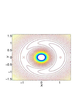
Figure 1: (Color online) Zero velocity surface contour plot at time $t=0$ for the hydrogen in the EP microwave electric field. $F=0.117,B=0$ (in scaled units). The circle (cross) indicates the location of the maximum (saddle) point of the ZVS.

Equation $(7)$ shows that the ZVS of the EP problem is not constant and oscillates around the origin with the frequency of the applied field. The linear stability analysis of equilibria performed in Lee97 for CP problem is not tractable for the EP problem. We study local dynamics around the Lagrange maximum by applying linear stability analysis rendered by the fast Lyapunov indicator (FLI) method.

III Description of the fast Lyapunov indicator method

To characterize the multidimensional phase space structures a method is needed that provides a clear representation of the chaotic and regular regions in the phase space, similarly to the pictures obtained by Poincaré sections. However for the three– and higher–dimensional systems the construction and visualization of Poincaré sections might be very complicated. An alternative is to define an indicator of chaoticity for each trajectory from a given subspace of phase space. Various diagnostics for different types of dynamical behavior are present in the literature; for instance, indicators of chaoticity are the characteristic Lyapunov exponent lich83 , the strength of diffusion of the instantaneous frequency in the frequency space laskar93 , the measure of complexity of the Fourier spectrum powell79 , and other available indicators that distinguish chaotic and regular dynamics cincotta00 ; cipriani98 . As a short–term dynamical diagnostic a method of Fast Lyapunov indicators (FLI) was proposed in Ref. froe97 to study weak chaos in high–dimensional systems. The main idea of the method is to study the evolution of the tangent vectors computed along a given trajectory of the system. This method has been applied to search for phase space structures in different types of problems: coupled standard maps guzz02 , celestial mechanics problems astakh04 , and vibrational dynamics of polyatomic molecules shch04 . In this paper we apply this method to the atomic system. Below we present a brief description of the method (for more details, see Ref. guzz02 ).

To obtain a numerical estimate on the growth of tangent vectors along the flow the equations of motion are integrated together with the corresponding equations for Jacobian matrix, i.e., we integrate the flow given by $f(X)$ and the tangent flow:

$$\frac{d}{dt}X=f(X)~{},\qquad\qquad\frac{d\mathcal{J}}{dt}=\mathcal{D}f(X)\mathcal{J}~{},$$ (10)

where $X=(x_{1},x_{2},\ldots,x_{n})$ is a $n$–dimensional vector in the phase space, $\mathcal{J}$ is $n\times n$ Jacobian matrix of the flow, $\mathcal{D}f(X)$ is the matrix of partial derivatives $\{\partial{f}_{i}/\partial{x}_{j}\}_{i,j=1,n}$ of the flow, and ${\mathcal{J}}(0)$ is the identity matrix. The columns of Jacobian matrix are the tangent vectors of the flow $\{{\bf v}_{j}\}_{j=1,n}$. Given initial tangent vector ${\bf v}_{0}$ for each initial condition ${\bf x}_{0}$ from the phase space of the system the fast Lyapunov indicator (FLI) is defined at time $t$ as follows:

$$\phi(t;{\bf x}_{0})=\max_{0\leq t^{\prime}\leq t}\log\|{\bf v}(t^{\prime};{\bf x}_{0})\|~{},$$ (11)

where ${\bf v}(t^{\prime};{\bf x}_{0})$ is the tangent vector at time $t^{\prime}$. For any initial choice of the tangent vector ${\bf v_{0}}$ it will eventually converge to the direction of the most unstable eigenvector of the Jacobian matrix $\mathcal{J}$. Hence, characteristic dynamics can be observed by integrating Eqs. $(10)$ for one of the tangent vectors from the set of all the tangent vectors in $\mathcal{J}$.

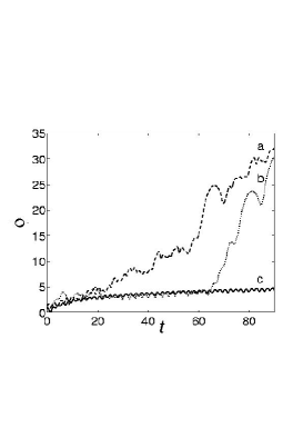
Figure 2: FLI curves for chaotic and regular trajectories of the hydrogen atom in a CP microwave field. $F=0.117,K_{max}=-1.3807,B=0$. Initial coordinates $(x,y)$ for the corresponding trajectories are: a) (1.5, 0.01), b) (0.9,0.01), and c) (0.8, 0.01). The values of the initial momenta are chosen as described in Sec. IV.1.1. The time $t$ is scaled and dimensionless.

The Lyapunov indicator defined in Eq. $(11)$ serves as an efficient diagnostic of chaoticity for any analyzed trajectory with initial condition ${\bf x}_{0}$. The FLI procedure supplies information about the dynamical behavior of a trajectory, analogously to the method of the characteristic Lyapunov exponents. The tangent vector growth evaluated by integration of Eq. $(10)$ is proportional to the growth of the distance between two neighboring trajectories in phase space. In fact, the evolution of the tangent vector computed for chaotic trajectories obeys an overall exponential law. Therefore, the FLI increases linearly in time. At the same time, the tangent vector growth for regular trajectories follows approximately a global linear behavior. Thus the FLI increases logarithmically in time. Already after a short interval of time it is possible to make a clear distinction between different dynamical behaviors of trajectories by looking at the maximum value attained by the FLI. To provide an example, in Fig. 2 the FLI evolution in time is shown for two chaotic and one regular trajectories from the phase space of the system defined by Hamiltonian $(5)$ . Already after a time $t=100$ two different types of dynamical behavior can be clearly identified. Meanwhile the curves $(a)$ and $(b)$ evolve almost linearly, the curve $(c)$ follows logarithmic growth with time. Note that $(b)$ and $(c)$ are launched very close and hence the FLI are very close for some time before they are distinguished since $(b)$ is chaotic and $(c)$ is regular (by inspections of their Poincaré sections)

The main advantage of FLI technique over other available methods is its power to discriminate regular from chaotic motions over a relatively short time period.

IV Numerical results

IV.1 Ionization dynamics at the maximum of zero–velocity surface

IV.1.1 Choice of initial conditions

We analyze the ionization dynamics of hydrogen atom in EP field by applying FLI stability analysis for trajectories from a mesh of initial conditions from the $x-y$ plane. For the CP problem we consider the subspace of initial conditions defined in Ref. Lee97 . Namely, the initial energy is chosen to be equal to the maximum of the ZVS: $K(0)=K_{max}$ as defined in Eq. $(9)$. The initial momenta $p_{x},p_{y}$ are chosen to satisfy the relation $p_{x}x+p_{y}y=0$.

For the CP problem the above defined subspace of initial conditions is two–dimensional and coincides with the two–dimensional Poincaré section. Similarly to the CP problem the dynamics for the EP problem is visualized on the $x-y$ plane. For the EP problem the effective Hamiltonian of the system has three degrees of freedom. In order to reduce the configuration space of the system to two–dimensional in five–dimensional energy subspace one needs to specify three initial conditions for coordinates and momenta. One condition is the same as for the CP problem. Additional conditions are defined by taking generalized coordinate $w=0$ and initial generalized momentum $p_{w}=-K(0)$.

IV.1.2 FLI analysis for CP and LP fields

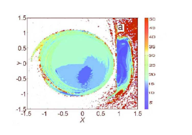
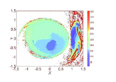
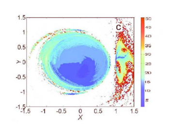
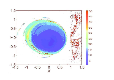
Figure 3: (Color online) FLI contour plots for hydrogen in a LP microwave field. Initial energy is equal to the maximum of the ZVS $K_{max}=-1.3807,B=0$. The scaled amplitudes of the electric field $F$ are: a) 0.117, b) 0.13, c) 0.16, and d) 0.2.

In this section the FLI stability results are presented for the LP field case. The magnetic field is zero. For each initial condition from the subspace defined in the previous section Eq. $(10)$ is integrated for a time $t=100$ (the time unit is one picosecond). The value of $\phi(t)$ in Eq. $(11)$ was evaluated at each moment of time. The maximum value attained over the integration interval $[0,100]$ is mapped onto the FLI plot. In Fig. 3 FLI contour plots are shown for several distinct amplitudes of the scaled LP electric field. The color code is assigned according to the maximum value of the FLI evaluated for each trajectory. The dark (blue in color version) color corresponds to the low values of the FLI and hence regular behavior; meanwhile the light (yellow and red) color indicates high values of the FLI and hence chaotic behavior. All the trajectories that ionize quickly are discarded and not marked on the plot (white regions). In addition, strongly chaotic trajectories with the value of the FLI greater than the critical value $\phi_{c}>50$ were discarded. In most cases strongly chaotic trajectories with $\phi(100)>50$ escape to infinity and ionize over the finite–time interval.

In the FLI contour plots presented in Fig. 3 two islands of stable motions can be clearly distinguished. In fact, a similar structure of the FLI plots exists for amplitudes of the electric field in the interval $[0.117,0.2]$. The central and right islands are located at the center and at the maximum of the ZVS respectively (see Fig. 1). The structure of the central island does not change with increasing amplitude of the field. This island is constituted by the bounded states that remain stable in a given range of the field amplitude. A layer of chaotic motions is located around the edges of the main stable islands. By comparing the FLI plots on Fig. 3 with the zero–velocity contour plot in Fig. 1 we observe that the stable island on the right hand side is located exactly in the vicinity of the Lagrange maximum of the ZVS. The area and the structure of the island change with increasing amplitude. The island remains almost the same for the field amplitudes $F=0.117$ and $F=0.13$. It shrinks at a field amplitude $F=0.16$ and completely disappears at $F=0.2$. These changes are the consequence of the break-up of invariant tori within the island. With increasing amplitude of the field they open paths for chaotic orbits to escape from the vicinity of the Lagrange maximum and to ionize.

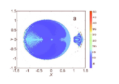
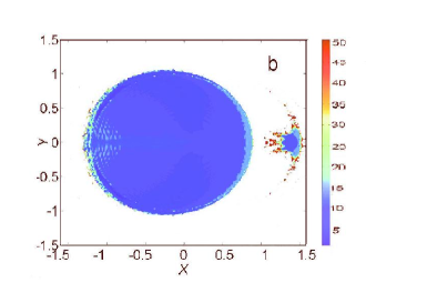
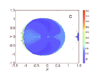
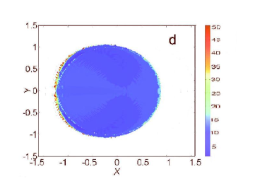
Figure 4: (Color online) FLI contour plots for hydrogen in a CP microwave field. Initial energy is equal to the maximum of the ZVS $K_{max}=-1.3807,B=0$. The color scale is assigned according to the values of the FLI. The scaled amplitudes of the electric field $F$ are: a) 0.117, b) 0.13, c) 0.14, and d) 0.15.

In Fig. 4 the FLI plots are shown for the CP problem. First, one observes that in all the four plots the size of the stability island around the Lagrange maximum is much smaller than the size of similar structures for the LP problem. Second, the size and structure of the central island look exactly the same as for the LP case. For the CP problem, the bounded states inside the central island remain stable for all the field amplitudes from the interval $[0.117,0.2]$. The field amplitude for which all the trajectories launched from the right hand side island ionize ($F=0.15$) is lower than the corresponding amplitude ($F=0.2$) for the LP case. As was mentioned before, for the CP field the system is time–independent in the rotating frame. The structures of the FLI contour plot coincide with the ones of the Poincaré section. As an example, in Fig. 5 the Trojan bifurcation is shown on the Poincaré section ($(a)$ panel) and on the FLI contour plot ($(b)$ panel). Figure 5$(b)$ is the magnification of the small island of Fig. 4$(a)$.

Figure 5: (Color online) The Poincaré surface of section and the magnification of the small island from Fig. 4$(a)$ are shown on panels $(a)$ and $(b)$ respectively.

A one–to–one correspondence of both plots is evident. On a close inspection, the symmetry about the $y$ axis is observed. The resonant zones on the Poincaré section correspond to the dark (blue in color version) islands on the FLI plot. The chaotic zones are marked around the edges of the islands.

To illustrate the FLI stability results, we show the ionization dynamics for the trajectories with the initial conditions inside two stable regions identified on the FLI plots and one trajectory with initial conditions inside the chaotic region. In Fig. 6 the configurations of three trajectories are shown as well as ZVS surface in the rotating frame. Initial conditions are chosen from different regions in Fig. 4: $(a)$ from the big stable island, $(b)$ from the small stable island, and $(c)$ from the chaotic region. Trajectories $(a)$ and $(b)$ correspond to the low eccentricity bounded states and trajectory $(c)$ is chaotic and ionizes after several close encounters with the nucleus.

IV.1.3 FLI analysis for EP field

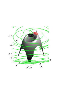
Figure 6: (Color online) Two stable orbits $(a)$, $(b)$, and one ionizing orbit $(c)$ versus the zero–velocity surface. The parameters are $K=K_{max},F=0.117,B=0$, and $\alpha=1$.

The FLI plots in Fig. 7 illustrate the structures for the hydrogen atom in EP field for the polarization degree $\alpha=0.6$. The scaled amplitude of the electric field is taken within the interval $[0.117,0.17]$. In general, the structure of the FLI plots for the EP field appears to be similar to the stability plots for the CP field case. Two islands of stability are apparent: a big island located at the center of ZVS and a small island located at the maximum of ZVS (see Fig. 1). The ellipticity of the field destroys the symmetry that is present for the CP field case. It is evident that the right hand side island in Fig. 7 $(c)$ is not symmetric around the $y$ axis as opposed to the ones around the maximum in Fig. 4. Lightly-colored regions can be seen on the edges of the two islands. These are initial conditions corresponding to chaotic trajectories with high values of the FLI. Trajectories with the values of the FLI higher than the critical $\phi_{c}=50$ are not represented. It can be observed that the large area surrounding the stable islands corresponds to rapidly ionizing chaotic motions. Similarly to the structure of the central island observed in Figs. 3 and 4, the equivalent structure for the EP field remains essentially unchanged with increasing strength of the field. At the same time noticeable changes are seen in the size and structure of the small island. The size of the small island varies substantially with the increase of the field amplitude. The growth of the island at certain amplitudes is accounted for the stabilization of some resonant motions within the island. For example, at $F=0.13$ the size of the island is noticeably larger than its size at $F=0.117$ in Fig. 7 $(a)$. At $F=0.17$ the small island disappears, i.e. most of the invariant tori within the island that existed at lower amplitudes of the field have been broken and almost all of the trajectories in the vicinity of the maximum become chaotic and ionize.

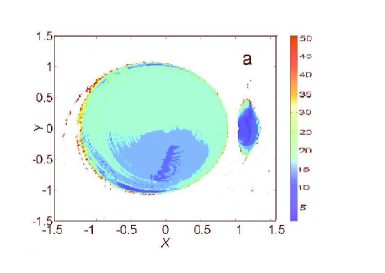
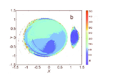
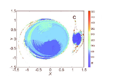
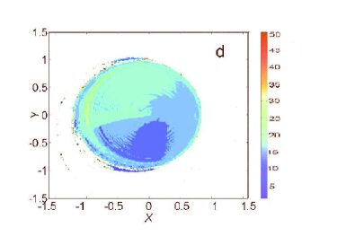
Figure 7: (Color online) FLI stability plots for hydrogen in EP microwave field. $K_{0}=K_{max},\alpha=0.6,B=0$. The scaled amplitudes of the electric field $F$ are: a) 0.117, b) 0.13, c) 0.15, and d) 0.17.

The FLI plots shows that the dynamics in the EP case is more regular than the CP case. For example, the size of the stable zone around the maximum point in Fig.  7 appears to be larger than the size of the stable zone in Fig. 4. On the other hand the size of the right hand side island in Fig. 7 for the EP field is much smaller than the size of the corresponding island in Fig. 3 for the LP field. From our detailed examination of the FLI results for the initial energy equal to the maximum of ZVS we conclude that the phase space dynamics is more regular for the LP field case than for the EP and CP field cases. Moreover, the size of the stable region around the Lagrange maximum point is observed to vary non–monotonically with the increase of the field amplitude for the EP field case. These changes are ascribed to various nonlinear resonant effects that were studied classically in Ref. rich97 and quantum mechanically using Floquet state approach in Ref. oks99 .

IV.2 Study of ionization probability curves

It has been pointed out in Ref. farrelly95 that the apparent ionization threshold for Rydberg atoms in the CP microwave field must be determined by the fraction of orbits that undergo first transition to chaos. Such orbits are located outside of the ZVS and they represent the atomic states that can be easily populated in the experiment beller97 . In connection with these results we found the set of bounded orbits in the vicinity of the Lagrange maximum of the ZVS. These are the orbits that undergo the transition from a regular to chaotic behavior within the range of electric field amplitude $F\in[0.12,0.18]$. The FLI plots in Figs. 3, 4 and 7, which are computed for the linear ($\alpha=0$), circular ($\alpha=1$), and intermediate ($\alpha=0.6$) polarizations, illustrate the changes of the stability of these orbits. While the dynamics in the central island remain unaffected by the increase of the field, the orbits located near the Lagrange maximum become chaotic and ionize with the increase of the field amplitude. For this reason, we determine an apparent ionization threshold by measuring the fraction of chaotic orbits from the phase space volume enclosing the Lagrange maximum. The calculations of the ionization probabilities are carried out for the polarizations of the field from the circular to the linear limit ($0<\alpha<1$). The behavior of the ionization probabilities versus scaled electric field amplitude $F\in[0.12,0.18]$ is estimated by means of the FLI analysis.

By monitoring the evolution of the FLI along each integrated trajectory we count the number of chaotic trajectories with the FLI value equal or above the critical value $\phi_{c}=50$. All chaotic trajectories are considered as possible candidates for the classical ionization. Indeed, the absence of invariant tori outside of the two stable structures distinguished by the FLI analysis shows that all chaotic trajectories escape from the vicinity of the Lagrange maximum to a zone associated with the high classical action values. The FLI plots in Figs. 3,4 and 7 show that the phase space surrounding the island at the Lagrange maximum is chaotic. There are no stable structures (except the big stable island at the center) that can prevent the escape of chaotic trajectories and their subsequent ionization.

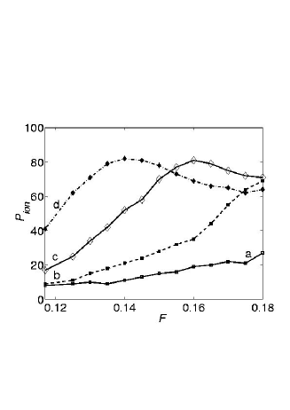
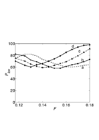
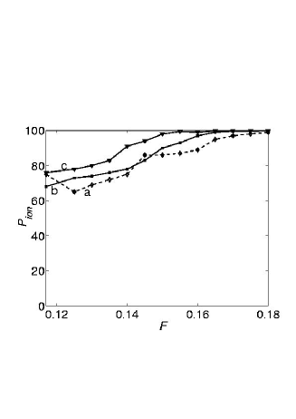
Figure 8: Ionization probability $P_{ion}$ computed for the ensemble of trajectories of hydrogen in EP microwave electric field. The parameters are $B=0,K(0)=K_{max}=-1.3807$. Top: ionization probabilities for the polarizations close to LP: a) 0, b) 0.1, c) 0.2, and d) 0.3. Center: Ionization probabilities for the intermediate polarizations: a) 0.4, b) 0.5, c) 0.6, and d) 0.7. Bottom: Ionization probabilities for the polarizations close to CP: a) 0.8, b) 0.9, and c) 1.

We define the percentage ionization probability from the ratio of the number of chaotic trajectories $N_{chaot}$ to the total number of trajectories $N_{total}$ from the volume of phase space surrounding the maximum point as follows:

$$P_{ion}=\frac{N_{chaot}}{N_{total}}\times 100\%.$$ (12)

The resulting apparent ionization probabilities versus the scaled field amplitude are shown in Fig. 8. Each curve represents the ionization probability for different field polarizations $\alpha$. On the top panel of Fig. 8 results are shown for the polarizations of the field close or equal to the LP limit. The curve $(a)$ indicates the percentage of chaotic trajectories in the vicinity of Lagrange maximum for the LP field. It is clearly seen that on average the percentage of chaotic trajectories within the phase space volume around the Lagrange maximum point is below $20\%$. The ionization probability $(a)$ increases slowly with the increase of the amplitude of the field. It is evident, that for the LP limit the dynamics around the Lagrange maximum remains predominantly regular for the electric field amplitude $F$ in the interval $[0.12,0.18]$. A qualitative illustration of the changes in dynamics for the LP limit is given in Fig. 3. From this figure one observes that transition from regular to chaotic dynamics occurs at $F=0.2$. On the top panel of Fig. 8 sharp changes in the behavior of the probabilities $(c)$ and $(d)$ are observed for the polarizations $\alpha=0.2$ and $\alpha=0.3$ respectively. First, the probabilities $(c)$ and $(d)$ rise rapidly from the $20\%$ and $40\%$ for $F=0.117$ to $80\%$ for the higher field amplitudes. Secondly, ionization probabilities $(c)$ and $(d)$ exhibit non–monotonic rise with the increasing field amplitude. Two pronounced local maxima in the ionization probabilities are observed for $F=0.16,~{}\alpha=0.2$ and for $F=0.14,~{}\alpha=0.3$. The main feature of the ionization probabilities seen on top panel is the sharp transition from almost monotonic behavior for $\alpha=0$ and $\alpha=0.1$ to the non–monotonic behavior for $\alpha=0.2$ and $\alpha=0.3$. This shows that dynamics around the Lagrange maximum strongly depends on the field polarization.

On the central panel the ionization probabilities are shown for intermediate polarizations. The behavior of the ionization probabilities is non–monotonic. For instance, there is a local maximum at $F=0.13$ and local minimum at $F=0.162$ for the curve $(a)$. The percentage of chaotic trajectories in the vicinity of the Lagrange maximum is equal to $80\%$. In fact, for the field amplitude $F=0.18$ and polarization $\alpha=0.6$ the percentage of chaotic trajectories is almost $90\%$, which means that most of the orbits around the Lagrange maximum ionize at these parameters of the field. These results were shown previously on the FLI stability plots in Fig. 7. Close inspection of the top and central panels shows that the probabilities for the higher polarizations are shifted to the left with respect to the probabilities for the lower polarizations. For example, the maximum for the $(a)$ probability from the central panel happens at $F=0.13$ and the maximum for the $(d)$ probability from the left panel occurs at $F=0.14$.

On the bottom panel of Fig. 8 the ionization probabilities are shown for polarizations of the field close to the CP limit. The fact that the ionization probabilities stay close to each other for polarizations $\alpha\in[0.8,1]$ demonstrates the lack of significant variations of dynamics in the vicinity of the Lagrange maximum. The probabilities change from the $80\%$ for $F=0.12$ up to $100\%$ for $F=0.18$. Moreover, the ionization curves follow almost monotonic growth with the increase of the amplitude of the field. For the CP limit all the trajectories around the Lagrange maximum become chaotic and ionize for $F=0.15$. This is the lowest ionization bound observed.

IV.3 Phase space dynamics below the saddle point of zero–velocity surface

In this section we discuss the FLI stability results for the ensemble of states with initial energy below the ZVS saddle point. In addition, non-zero constant magnetic field was applied perpendicular to the plane of polarization.

Previously it has been shown that the application of a magnetic field perpendicular to the polarization plane leads to stabilization of some of the phase space invariant tori for hydrogen in a CP field Lee97 ; chand02 . In turn, the invariant tori create barriers to the diffusion of chaotic trajectories within the phase space. In this section we perform FLI stability analysis for the hydrogen in EP microwave field and non–zero magnetic field. As a starting point, the FLI stability analysis is applied to hydrogen in CP field for the same parameters of the electric and magnetic fields. The FLI calculations are carried out on a grid of points from the $x-y$ plane for magnetic field $B=0.2$ and initial energy $K_{0}=-2$ (the saddle point value of the ZVS is $K_{sad}=-1.7022$). The resulting FLI stability plots are shown in Fig. 9.

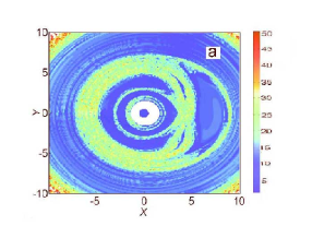
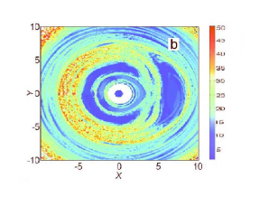
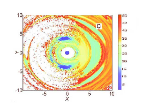
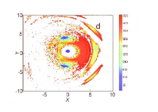
Figure 9: (Color online) FLI stability plots for hydrogen in an EP microwave field. $F=0.117,B=0.2,K=-2$. The polarization of the field is : a) 1, b) 0.8, c) 0.5, and d) 0.3. The color scale is assigned according to the maximum values of the FLI attained over the integration interval $t=100$.

On panel $(a)$ the structure of the phase space is shown for the CP field. Note the dark (blue in color version) island of stability around the nucleus. The same stable island was observed in Figs. 3, 4 and 7. It is located around the center of the ZVS. The island is surrounded by the classically inaccessible region. The phase space outside of the region is foliated with regular and chaotic motions. Chaotic dynamics is associated with high values of the FLI and color coded with light colors (yellow and red in color version). The large resonant zone is located on the right from the center of the FLI plot. The phase space appears to be mostly regular, except for thin chaotic layers winding around the large resonant zones. It is easy to notice that the structure is symmetric with respect to the $y$ axis. On panel $(b)$ the phase space dynamics is pictured for the polarization $\alpha=0.8$. The structure resembles the one shown on panel $(a)$: the FLI plot shows the same resonant structures and chaotic layers as those observed on panel $(a)$. However, the overall dynamics appear more chaotic than for the CP field case. The stability results for the intermediate polarizations $\alpha=0.5$ and $\alpha=0.3$ are shown on the panels $(c)$ and $(d)$ correspondingly. The phase space dynamics on both panels appear to be much more chaotic than the dynamics for the CP limit. Although the large part of the phase space on contour plots $(c)$ and $(d)$ corresponds to strongly chaotic motions, several stable islands can be distinguished. For example, two small islands of stability are located symmetrically with respect to the $y$ axis.

Our main observation from the FLI stability results described in this section is that the application of magnetic field leads to the stabilization of the resonant structures within the phase space of the system. The FLI plots reflect the onset of stochasticity in the phase space of the system that occurs when the field polarization approaches LP limit. The phase space structure appears to be more regular for the field polarizations close to the CP limit as opposed to the polarizations close to the LP limit.

IV.4 Description of an ensemble of initial states and comparison with the stability analysis results

Finally, in this section we introduce the classification of the ensemble of orbits used for the FLI stability calculations in the previous sections. In the experiment beller97 the ensemble of initial states are prepared spanning a narrow range of the Keplerian energy $E=-\frac{1}{2n^{2}}$ and a variety of high eccentricity orbits. As the field is turned on, the states with the same action $n$ will appear in different regions of the phase space having different values of energy and eccentricities $\epsilon=\sqrt{1-l_{z}^{2}/n^{2}}$ ($l_{z}$ is angular momentum) in the rotating frame. While the Hamiltonian dynamics is traditionally studied by restricting the phase space to the constant energy manifold, one would ideally prefer to relate numerical results with the experiment and to study an ensemble of states with the same Keplerian energy. However, most of the numerical simulations based on the examining the structure of the Poincaré section use trajectories with different values of the Keplerian energy $K$. For the FLI stability analysis we use an ensemble of initial states with equal initial energies $K(0)$ and different values of initial action $n$ and eccentricity $\epsilon$. We choose these initial states to compare the stability pictures given by the FLI method with the Poincaré sections.

The interpretation of numerical results and comparison with experiments is much more complicated for the EP problem. The presence of the time–dependent term in the expression of the Hamiltonian in the rotating frame prevents the one-to-one relation between the initial state (at time $t=0$) and the final state (obtained after the turn–on of the field). Therefore, it is instructive to relate the FLI stability results for the ensemble of states analyzed with their initial eccentricities, actions and angular momenta. The importance of the configuration of initial states in the ionization mechanism was realized, e.g., in Refs. kappertz93 ; farrelly95 ; brunello96 . We found that our results agree in their key features with the conclusion stressed out in Ref. brunello96 : the fate of the initial states subjected to the application of the field cannot be predicted from the initial action values and eccentricities of such states. In essence, the states with the same initial action and eccentricity values can be moved by the application of the field to different parts of the phase space. We illustrate these conclusions by comparing the FLI stability results given in Secs. IV.1 and IV.3 with the configuration of initial states involved in the FLI computations.

Figure 10: The action variable $n$, angular momentum $l_{z}$, and eccentricity $\epsilon$ of the initial states of hydrogen in the EP microwave field are shown on panels $(a),(b),$ and $(c)$ correspondingly. The parameters are $F=0.117,K_{max}=-1.3807$, and $B=0$.

First, we analyze the ensemble of states with initial energy equal to the maximum of the ZVS. In Fig. 10 the action variables $n$, angular momenta $l_{z}$ and eccentricities $\epsilon$ are computed for the ensemble of initial states used for the FLI stability analysis in Sec. IV.1. The case of zero magnetic field is considered. The scaled amplitude of the electric field is $F=0.117$, polarization is $\alpha=1$, and the initial energy value is equal to the maximum $K_{max}=-1.3807$ of the ZVS defined in Eq. $(9)$. On panel $(b)$ the values of initial angular momentum $l_{z}$ are shown. It can be seen from Fig. 10$(b)$ and FLI plots in Fig. 7 that the states inside the central stable island correspond to negative angular momentum states. The rest of the trajectories in the FLI plots in Fig. 7 corresponds to positive angular momentum initial states. Another important observation is that the central stable island is associated with bounded states of different eccentricities. From the stability results given in Sec. IV.1 these states remain bounded for the range of the scaled field amplitude $[0.117,0.2]$ and for different polarizations of the field. From Fig. 10$(c)$ and FLI plots in Fig. 7 it is apparent that the initial states around the maximum of ZVS are the low eccentricity states. In fact, these are the states that determine the low ionization threshold computed in Sec. IV.2. Summarizing data given in Figs. 7 and 10 we argue that the ultimate fate of initially low eccentricity and positive angular momentum states is to be moved by the driving field to the chaotic region of the phase space and undergo fast ionization. At the same time, the initial states with negative value of angular momentum located around the center of the ZVS remain bounded.

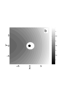
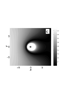
Figure 11: The action variable $n$, angular momentum $l_{z}$, and eccentricity $\epsilon$ of the initial states of hydrogen in the EP microwave field are shown on panels $(a),(b),$ and $(c)$ correspondingly. The parameters are $F=0.117,K=-2$, and $B=0.2$. The initial energy of the states $K$ is taken below the saddle point energy $K_{sad}=-1.7022$.

Next, we classify the initial states with energy below the saddle point of the ZVS. In Fig. 11 the action, angular momentum and eccentricity together with the FLI plot are presented for the initial states of hydrogen subject to EP field $F=0.117$ with polarization $\alpha=0.9$ and magnetic field $B=0.2$. The initial energy $K(0)=-2$ is chosen below the saddle point $K_{sad}=-1.7022$ of the ZVS. The main conclusion from the data given in Figs. 9 and  11 is that the initial states with low eccentricity tend to be more stable than the states with high eccentricity values. For example, from Fig. 9$(d)$ one observes three small stable islands with low values of the FLI: one island is around the center of ZVS and the other two islands are symmetric with respect to the $y$–axis. Two symmetric islands correspond to low eccentricity states in Fig. 11$(c)$.

The comparison of data presented in this section with the stability results given by FLI analysis show that, although the fate of initial states can be determined from their eccentricity and angular momentum values in some cases, in general, this information is not sufficient for predicting the dynamics of the states after the turn–on of the field. Instead, the analysis of the character of the states should be performed in conjunction with the stability analysis.

V Conclusions

In this article, we provide a qualitative description of the classical phase space and its relevance to the ionization of hydrogen atom in a strong EP microwave field. Using the FLI stability analysis, the complex multidimensional dynamics is shown to depend sensitively on the changes of parameters including polarization, amplitude of the electric and magnetic fields and the initial state ensemble. The FLI stability analysis allows us to picture complex phase space structures, such as important resonant and chaotic zones.

We map out the FLI values for each trajectory originating on the zero–velocity subspace for the ensemble of orbits with initial energy at the maximum of the ZVS. Our FLI stability computations for the LP and CP fields reveal two main resonant structures: a small stable island around the Lagrange maximum of the ZVS and a large stable island around the center of the ZVS. The small stable island corresponds to the initial states with low eccentricity values and positive angular momenta. In contrast, the initial states from large stable island are the negative angular momentum states with different eccentricity values. These states remain bounded and their dynamics is almost unaffected by the application of the microwave field. The remaining part of phase space is attributed to chaotic motions that ionize quickly over the interval of time considered in the computations. The main feature of FLI stability results is that the ionization dynamics is determined by the orbits with low eccentricity and positive momentum states located around the maximum of the ZVS. These states are the first to become chaotic and ionize for a given strength of the field. Similar observations hold for the EP field case: The FLI plots reflect stable structures similar to those observed for the LP and CP problems. The main distinction from the LP and CP field results is the behavior of stable island around the Lagrange maximum. It changes non–monotonically with the increase of the amplitude of the electric field due to break–up and stabilization of resonant torus structures within the island.

Our main conclusion is that the nonlinear stability of the Lagrange maximum is determined by the parameters of the field, such as the amplitude of electric and magnetic field as well as the field polarization. The ionization probabilities versus the amplitude of the electric field reflect the changes in the local dynamics around the Lagrange maximum. They manifest non–monotonic growth for intermediate ellipticities of the field. This behavior agrees with the experimentally observed ionization yields in Ref.  beller97 .

The FLI stability analysis was also carried out for the ensemble of states with initial energy below the saddle value of the ZVS. In this case the FLI plots reflect the onset of stochasticity in phase space that takes place as the field polarization changes from the circular to the linear limit. The FLI simulations reveal the detailed structure of phase space that is more regular for the field polarizations close to the circular limit as opposed to the polarizations close to the linear limit.

The application of the method can be potentially important for the control of ionization of Rydberg states in recent experiments  sirko02 . The main advantage of this technique over other available analytical and numerical methods is its independence from the dimensionality of the system. Thus, the stability analysis can be carried out for any subspace of initial conditions in the full–dimensional phase space of the system.

The method can be useful for estimating the size of a stable zone around the equilibria for the wave packet calculations and stabilization of quantum wave packets at the Lagrange equilibria points discussed in Ref. Lee97 . We expect that by varying polarization and amplitude of electric and magnetic fields, one can achieve the stabilization of a set of resonances around the Lagrange maximum that can possibly lead to the stabilization of the quantum wave packets in the EP field system.

- (1) J. E. Bayfield and P. M. Koch, Phys. Rev. Lett. 33, 258 (1974).
- (2) P. M. Koch and K. A. H. van Leeuwen, Phys. Rep. 255, 289 (1995).
- (3) M. R. W. Bellermann, P. M. Koch and D. Richards, Phys. Rev. Lett. 78, 3840 (1997).
- (4) H. Maeda and T. F. Gallagher, Phy. Rev. Lett. 93, 133004 (2004).
- (5) A. Brunello, T. Uzer and D. Farrelly D, Phys. Rev. Lett. A 55, 3730 (1997).
- (6) M. R. W. Bellermann, P. M. Koch, D. R. Mariarni and D. Richards, Phys. Rev. Lett. 76, 892 (1996).
- (7) D. Richards, J. Phys. B : At. Mol. Opt. Phys. 30, 4019 (1997).
- (8) E. A. Oks and V. P. Gavrilenko, Opt. Commun. 46, 205 (1983).
- (9) E. Oks and T. Uzer, J. Phys. B : At. Mol. Opt. Phys. 32, 3601 (1999).
- (10) Panming Fu, T. J. Scholz, J. M. Hettema, and T. F. Gallagher, Phys. Rev. Lett. 64, 511 (1990).
- (11) J. A. Griffiths and D. Farrelly, Phys. Rev. A 45, R2678 (1992).
- (12) P. Kappertz and M. Nauenberg, Phys. Rev. A. 47, 4749 (1993).
- (13) C. Froeschlé, E. Lega and R. Gonczi, Celest. Mech. Dyn. Astron. 67, 41 (1997).
- (14) E. Shchekinova , C. Chandre, Y. Lan and T. Uzer, J. Chem. Phys. 121, 3471 (2004).
- (15) H. Salwen, Phys. Rev. 99, 1274 (1955).
- (16) V. I. Arnold, Mathematical methods of classical mechanics, (Springer–Verlag, New York, 1989).
- (17) J. von Milczewski, G. H. F. Diercksen, and T. Uzer, Phys. Rev. Lett. 76, 2890 (1996).
- (18) D. Farrelly and T. Uzer, Phys. Rev. Lett. 74, 1720 (1995).
- (19) C. Chandre, D. Farrelly and T. Uzer, Phys. Rev. A 65, 053402 (2002).
- (20) B. V. Chirikov, Phys. Rep. 52, 263 (1979).
- (21) G. Casati, B. V. Chirikov, D. L. Shepelyansky, and I. Guarnieri, Phys. Rep. 154, 77 (1987).
- (22) R. V. Jensen, Phys. Rev. A 30, 386 (1984).
- (23) J. E. Howard, Phys. Rev. A 46, 364 (1992).
- (24) R. Blümel, Phys. Rev. A 49, 4787 (1994).
- (25) K. Sacha and J. Zakrzewski, Phys. Rev. A 30, 568 (1997).
- (26) I. Bialynicki–Birula, M. Kaliński and J. H. Eberly, Phys. Rev. Lett. 73, 1777 (1994).
- (27) A. F. Brunello, T. Uzer and D. Farrelly, Phys. Rev. Lett. 76, 2874 (1996).
- (28) E. Lee, A. F. Brunello and D. Farrelly, Phys. Rev. Lett. 75, 3641 (1997).
- (29) G. W. Hill, Am. J. Math. 1, 5 (1878).
- (30) V. Szebehely, Theory of Orbits: The Restricted Problem of Three Bodies, (Academic, New York and London, 1967).
- (31) A. J. Lichtenberg and M. A. Lieberman, Regular and Stochastic Motion (Springer–Verlag, New York, 1983).
- (32) J. Laskar, Physica D 67, 257 (1993).
- (33) G. E. Powell and I. C. Percival, J. Phys. A.12, 2053 (1979).
- (34) P. Cincotta and S. Simó, Astron.& Astrophys. 147, 205 (2000).
- (35) P. Cipriani and M. Bari, Planet. Space Science, 46, 1543 (1998).
- (36) M. Guzzo, E. Lega and C. Froeschlé, Physica D 163, 1 (2002).
- (37) S. A. Astakhov and D. Farrelly, Mon. Not. R. Astron. Soc. 354, 971 (2004).
- (38) L. Sirko and P. M. Koch, Phys. Rev. Lett. 89, 274101 (2002).