Formation and evolution of singularities in anisotropic geometric continua

Abstract.

Evolutionary PDEs for geometric order parameters that admit propagating singular solutions are introduced and discussed. These singular solutions arise as a result of the competition between nonlinear and nonlocal processes in various familiar vector spaces. Several examples are given. The motivating example is the directed self assembly of a large number of particles for technological purposes such as nano-science processes, in which the particle interactions are anisotropic. This application leads to the derivation and analysis of gradient flow equations on Lie algebra valued densities. The Riemannian structure of these gradient flow equations is also discussed.

1. Introduction

Many physical processes may be understood as aggregation of individual ‘components’ at a variety of scales into a final ‘product’. Diverse examples of such processes include the formation of stars, galaxies and solar systems at large scales, organization of insects and organisms into colonies at mesoscales and self-assembly of proteins, nanotubes or micro/nanodevices at micro- and nanoscales [1]. Some of these processes, such as nano-scale self-assembly of molecules and particles are of great technological interest [2, 3]. In most practical cases, the assembling pieces do not have spherical symmetry, and the interaction between those pieces is not central, i.e., it is dependent not only on the density of the particles, but also on their mutual orientation. A recent example, motivating this paper, is self-assembly of non-circular floating particles (squares, hexagons etc.) [4, 5, 6]. Due to the large number of particles involved in self-assembly for technological purposes, ($10^{9}-10^{12}$), the development of continuum descriptions for aggregation or self-assembly is a natural approach toward theoretical understanding and modeling.

Progress has been made recently in the derivation of continuum evolutionary equations for self-assembly of molecules evolving under a long-range central interaction potential. The resulting continuum models emerge in a class of partial differential equations (PDEs) that are both nonlinear and nonlocal [7, 8]. Nonlinearity and nolocality may combine in an evolutionary process to form coherent singular structures that propagate and interact amongst themselves. Thus, self-assembly is modeled in the continuum description as the emergent formation of singular solutions. Classic examples of equations admitting such singular solution behavior include the Poisson-Smoluchowsi (PS) equation [9], Debye-Hückel equations [10] and the Keller-Segel (KS) system of equations [11]. PS and KS are gradient flows for densities that collapse to subspaces in finite time. Their respective collapses model the formation of clumps from randomly walking sticky particles (PS) and the development of concentrated biological patterns via chemotaxis (KS). For recent thorough review and references, see [12]. A variant of these equations of potential use in modeling formation of clustering in biology (e.g., formation of herds of antelope, or schools of fish) was introduced in Bertozzi and Topaz [13]. Dynamics and collapse of self-gravitating systems has been studied by Chavanis, Rosier and Sire [14]. Finally, aggregation of particles with the applications to directed self-assembly in nanoscience was considered by Holm and Putkaradze (HP) in [7, 8]. The singular solutions of the latter HP equation emerge as delta functions supported on a subspace from smooth initial conditions. These clumps or “clumpons” then propagate and interact by aggregating into larger (more massive) clumps when they collide. See also [15] for a thoughtful discussion of singularity formation in fundamental mathematical terms.

Remarkably, the aggregation and emergence of singular solutions from smooth initial data due to nonlinearity and nonlocality need not be dissipative. A Hamiltonian example is provided by the Camassa-Holm (CH) equation for shallow water waves in its limit of zero linear dispersion [16]. In this limit, the CH equation describes geodesic motion on the Lie group of smooth invertible maps with smooth inverses (the diffeomorphisms, or diffeos, for short) with respect to the $H^{1}$ Sobolev metric. Being an integrable Hamiltonian system, the CH equation has soliton solutions which emerge in its initial value problem. In its dispersionless limit these CH soliton solutions develop a sharp peak at which the derivative is discontinuous, so the second derivative is singular. At the positions of these propagating peaks (the peakons), the momentum density is concentrated into delta functions. The CH peakons propagate and interact elastically by exchanging momentum; so they bounce off each other when they collide.

CH arises as an Euler-Poincaré (EP) equation from Hamilton’s principle defined using a Lagrangian which is right-invariant under the action of the diffeos on their own Lie algebra (the tangent space at the identity) [17]. In the EP approach, variations in Hamilton’s principle of the vectors in linear representation spaces of the group of diffeos are induced from variations of the diffeos themselves. Hence these variations in the EP Hamilton’s principle arise as geometrical operations, primarily as Lie derivatives of elements of the appropriate linear representation spaces. Moreover, evolution by CH – or more generally by any of the class of EP equations on the diffeos (EPDiff) – is by coadjoint action of the diffeos on the momentum density. This infinitesimal action is defined as the Lie derivative of momentum density by its corresponding velocity vector field. The momentum density for a singular solution of CH is supported on its singular set, regarded as an embedded submanifold [18].

CH and other equations in the class of EPDiff equations hint that the actions of diffeos may be taken as a paradigm for the development and propagation of singularities in other geometrical quantities, or at least would provide a framework for studying the process and discovering additional examples of it. In fact, the HP equation was discovered by following Otto [19] in formulating the process of nonlinear nonlocal evolution using a variational principle in which the variations were induced by the infinitesimal actions of diffeos on densities [7, 8]. Just as in Hamilton’s principle for the EP equations, this infinitesimal action is the Lie derivative with respect to a vector field and for HP the vector field was related by Darcy’s Law to the flux of density.

The derivation of evolution equations for density in the framework of Darcy’s law is now well established: The velocity of a particle is taken to be proportional to the force acting on it, and the conservation law for density $\rho$ readily establishes a PDE for its evolution. The Darcy law evolution equation for density corresponds to conservation of the $n$-form in $n$-dimensional space $\rho\mbox{d}^{n}\mathbf{x}$ along characteristics of a velocity determined from the density and its gradient. Physically, the conservation law for $\rho\mbox{d}^{n}\mathbf{x}$ means preservation of the number of particles, or mass, in an infinitesimal volume.

The density evolution equation closes if the potential of interaction between the particles depends only on their relative position. This framework is simple and attractive. However, the energy of some physical systems depends strongly on additional geometric quantities, such as the mutual orientations of their pieces. Examples of such systems are numerous and range from micro-biological applications (mutual attraction of cells, viruses or proteins), to electromagnetic media (dipoles in continuous media, orientation of domains), to interaction of living organisms [1].

Summary of the paper. This paper provides a new geometric framework for continuum evolutionary models of particle systems whose interactions depend on orientation. Interestingly enough, this framework is completely general and can be applied to the evolution of any geometric quantity. The problems which involve both density and orientation are perhaps the most intricate, and for pedagogical reasons we shall treat them towards the end of the paper, after we have first illustrated the general framework by treating the familiar cases of scalars and 3-forms (particle densities).

After this preparation establishing the pattern for the results in simpler cases, we shall derive the covariant evolution equation (9.7) for quantities which depend on both particle densities and orientations. In this framework, one may use the same principles in deriving evolution equations for any geometric quantity. Of course, the forms of the various evolution equations will strongly depend on what geometric quantity is being considered.

Once the equations of motions for the geometric quantities are derived, we shall concentrate on the establishment of singular analytical solutions of these equations. Earlier work for the case of density evolution [7, 8] demonstrated that when such solutions exist, they play a dominant role in the dynamics. Thus, we seek additional examples of the formation of coherent, propagating singularities in solutions of evolutionary PDEs. These singularities arise as a result of the competition between nonlinear and nonlocal processes in various familiar vector spaces. We follow the same strategy as [7, 8] in taking variations of a free energy that are induced by infinitesimal actions of diffeos on these vector spaces. To close the equations, we also introduce a geometric analog of Darcy’s Law, based on the dual representation of these actions. This approach yields several other nonlinear nonlocal PDEs whose solutions form coherent propagating singular structures in finite time. The present approach should be useful whenever geometry figures in the formation and evolution of moving singularities. However, the development of this approach is only beginning and the full extent of its applications remains to be proven. Besides the applications mentioned earlier, see for example, the spontaneous formation of singularities (self-focusing) in the spin wave turbulence [20].

Plan. The plan of the paper is the following. Section 2 reviews earlier work on the gradient flow evolution for density and formulates the geometric order parameter (GOP) equation. This formulation summons the diamond operator from differential geometry, whose properties are discussed in Section 3. Section 4 introduces a necessary condition for the existence of singular solutions of GOP equations in the general case. Applications require explicit calculation of the diamond operator for each geometric quantity, which is accomplished in Section 5. Section 6 derives explicit expressions for GOP equations of motion and Section 7 gives examples of singular solutions. Finally, Section 8 is devoted to the equations of motion for orientation densities whose Lie-algebra-valued singular solutions are called gyrons. We also compare the results of our theory to recent experiments on self-organization of oriented particles.

2. Problem statement

We consider continuum evolution of the macroscopic state of a system of many particles at time $t$ and position $\boldsymbol{x}$ that is defined by an order parameter $\kappa(\boldsymbol{x},t)$, which take values in a vector space $V$. The vector space has a dual space $V^{*}$, defined in terms of the $L^{2}$ pairing

$$\langle\boldsymbol{\cdot}\,,\,\boldsymbol{\cdot}\rangle:\,V\times{V^{*}}\mapsto\mathbb{R}\,.$$

For example, scalar functions are dual to densities, one-forms are dual to two-forms and vector fields are dual to one-form densities.

In addition, we assume that the physical situation dictates a free energy, which is a functional of the order parameter expressed as $E[\kappa]$, where square brackets $[\,\cdot\,]$ denote dependence which may be spatially nonlocal. That is, $E[\kappa]$ may also be a functional of $\kappa$; for example, it could depend on the spatially averaged or filtered value of $\kappa$ defined later. Hence, the variation of total integrated energy is given by the pairing,

$$\delta E[\kappa]=\bigg{\langle}\delta\kappa\,,\,\frac{\delta E}{\delta\kappa}\bigg{\rangle}=\int\delta\kappa\cdot\frac{\delta E}{\delta\kappa}\,,$$

where dot $(\,\cdot\,)$ denotes the appropriate pairing of vector and covector indices of $\kappa$ to produce a density, an $n-$form (denoted as $\Lambda^{n}$) which then may be integrated to yield a real number. Of course, $n$ is the dimension of the space. In this paper, we shall concentrate on the cases $n=1,2,3$. In this setting, we seek evolution equations for the order parameter $\kappa(\boldsymbol{x},t)$ that
(1) respect its vector space property $\kappa\in V$;
(2) reduce to gradient flows when $\kappa$ is a density; and
(3) possess solutions that may aggregate the order parameter $\kappa$ into “clumpons” (quenched states) which propagate and interact as singular weak solutions.

Thus we seek evolution equations whose solutions describe a geometric order parameter supported on embedded subspaces of the ambient space. For example, these solutions may be spatially distributed on curves in 2D, or on surfaces in 3D. In fact, we seek evolution equations for which these embedded singular solutions are attractors which emerge even from arbitrary smooth initial conditions, as in the case of the emergent singular densities for the nonlocal gradient flows studied in [7, 8]. Our ultimate goal is to find classes of equations that are relevant for the evolution of a macroscopic order parameter that may be of potential use in the design of directed self-assembly processes in nanoscience.

Previous work focused on emergent singularities in an order parameter density [7, 8]. These singularities correspond to the formation of dense clumps of maximum possible density in self-assembly of nano-particles. Two different cases were distinguished in the model. The first case arises when the mobility of the particles $\mu$ always remains finite, in which case the evolution forces the particles to collapse into a set of $\delta$-functions. These $\delta$-functions can be understood as a large-scale view of individual clumps. The second case arises upon modeling the clumping process in greater detail, by limiting the mobility so that it will eventually decrease to zero at some maximal value of averaged density. This leads to formation of patches of constant density. (See also [21] for the case of density-dependent mobility.) In the next section, we shall cast the results of previous work into the geometric framework taken here in the derivation of the equations.

2.1. An example: the HP equation for the gradient flow of a density

      

Holm and Putkaradze [7, 8] derived the HP gradient flow, whose singular densities (the clumpons) emerge in finite time for any smooth initial conditions possessing a maximum density. The HP equation is the gradient flow of a density $\rho\in\Lambda^{n}$ given by

(2.1) $$\frac{\partial\rho}{\partial t}=-\,{\rm div}\,\bigg{(}\rho\mu[\rho]\,\nabla\,\frac{\delta E}{\delta\rho}\bigg{)}\,.$$

Equation (2.1) has a clear physical meaning as follows. A potential at a given point $\delta E/\delta\rho$ gives rise to the force $\nabla(\delta E/\delta\rho)$. The particles move with covariant velocity $\eta$ proportional to the force applied to them. The mobility $\mu$ gives the coefficient of proportionality. Thus, the instantaneous contravariant velocity at a given point is

(2.2) $$\eta=\left(\mu\nabla\delta E/\delta\rho\right)^{\sharp}.$$

The familiar musical operations sharp $(\sharp)$ and flat $(\flat)$ raise and lower vector indices, respectively, thereby mapping a covector into a contravector and vice versa, as needed for the operations of divergence, Lie derivative, etc. to make proper mathematical sense. In particular, the contravariant velocity $\mathbf{u}$ advects the particle density according to

(2.3) $$\frac{\partial\rho}{\partial t}=-\,\pounds_{(\mu{\nabla}\frac{\delta E}{\delta\rho})^{\sharp}}\rho\,,$$

which provides the geometric meaning of the HP evolution equation (2.1).

In the traditional framework, each extensive quantity is assumed to be conserved, so its density per unit volume $\rho$ satisfies the continuity equation

(2.4) $$\frac{\partial\rho}{\partial t}=-\,{\rm div}\,\mathbf{J}\,,$$

where $\mathbf{J}$ is the flux density of the conserved quantity. This flux density is assumed to be proportional to the density of the extensive quantity. It is also taken to be proportional to the gradient of the thermodynamic conjugate variable $\delta E/\delta\rho$ in the First Law for specific energy $E$, modified to be contravariant so that its divergence may be properly defined. Thus the name, “gradient flow.” Finally, a phenomenological characterization of the freedom of motion of the particles is introduced, called their “mobility” $\mu[\rho]$, which transforms as $\rho$. Thus, one finds the Darcy Law for flow through a porous medium, for example, as,

(2.5) $$\mathbf{J}=\rho\,\Big{(}\mu\,\nabla\,\frac{\delta E}{\delta\rho}\Big{)}^{\sharp}\,.$$

By this thermodynamic reasoning one recovers the HP equation (2.1), from the continuity equation (2.4) and the definition of mobility in Darcy’s Law (2.5). As a consequence, the energy $E[\rho]$ evolves according to

(2.6) $$\frac{dE}{dt} = \bigg{\langle}\,\Big{(}\mu\,\nabla\,\frac{\delta E}{\delta\rho}\Big{)}^{\sharp},\,\Big{(}\rho\,\nabla\,\frac{\delta E}{\delta\rho}\Big{)}\bigg{\rangle}$$

$$= \int\rho\,\mu[\rho]\Big{|}\nabla\,\frac{\delta E}{\delta\rho}\Big{|}^{2}\,d\,^{n}x=\int\frac{1}{\rho\mu[\rho]}\big{|}\mathbf{J}\big{|}^{2}\,d\,^{n}x\,.$$

Note that for attracting particles, $E<0$, so the absolute value of energy decays in time $d|E|/dt<0$ when $\rho\,\mu[\rho]>0$.

Holm and Putkaradze [7, 8] analyzed the solutions of the gradient flow (2.1) when the mobility density $\mu[\overline{\rho}]$ depended on the spatially averaged density $\overline{\rho}=H*\rho$, defined as the convolution of density $\rho$ with the kernel $H$. The latter was chosen to be the Green’s function for the Helmholtz operator. The energy density was chosen in [7, 8] so that $\delta E/\delta\rho=G*\rho$, where $G$ was a Helmholtz kernel whose scale length is larger than that for $H$. Thus, $\delta E/\delta\rho$ depended on the average density at the lengthscale of $G$, rather than the pointwise density.

With these choices, the solution $\rho$ of the HP gradient flow, paired with a smooth scalar test function $\phi$ satisfies

$$\Big{\langle}\frac{\partial\rho}{\partial t}\,,\,\phi\Big{\rangle} = \Big{\langle}-\,{\rm div}\,\bigg{(}\rho\Big{(}\mu[\overline{\rho}]\,\nabla\,\frac{\delta E}{\delta\rho}\Big{)}^{\sharp}\bigg{)}\,,\,\phi\Big{\rangle}$$

$$= \Big{\langle}\rho\Big{(}\mu[\overline{\rho}]\,\nabla\,\frac{\delta E}{\delta\rho}\Big{)}^{\sharp}\,,\,\nabla\phi\Big{\rangle}$$

$$= \Big{\langle}\rho\,,\,\Big{(}\mu[\overline{\rho}]\,\nabla\,\frac{\delta E}{\delta\rho}\Big{)}^{\sharp}\cdot\nabla\phi\Big{\rangle}$$

$$= \Big{\langle}\rho\,,\,\pounds_{(\mu[\overline{\rho}]\,\nabla\,\frac{\delta E}{\delta\rho})^{\sharp}}\,\phi\Big{\rangle}\,.$$

Under the the $L^{2}$ pairing $\langle\boldsymbol{\cdot}\,,\,\boldsymbol{\cdot}\rangle$, the third line matches with the derivative of a delta function; so the HP gradient flow admits singular solutions.

2.2. Singular solutions for the HP gradient flow of a density

Provided $\mu[\overline{\rho}]$ and $\delta E/\delta\rho$ are sufficiently smooth, the HP equation (2.1) admits solutions $\rho$ that are sums of delta functions supported on $N$ manifolds of dimension $K_{a}$, $a=1,2,3,\dots,N$, with coordinates $s$ embedded in $\mathbb{R}^{3}$. Namely,

(2.7) $$\rho(\boldsymbol{x},t) = \sum_{a}\int_{s}p_{a}(t,s)\delta\big{(}\boldsymbol{x}-\boldsymbol{q}_{a}(t,{s})\big{)}\,ds\,,$$

(2.8) $$\overline{\rho}(\boldsymbol{x},t) = H*\rho=\int H(\boldsymbol{x},\boldsymbol{x}^{\prime})\rho(\boldsymbol{x}^{\prime})\,d\,^{3}x^{\prime}$$

$$= \sum_{a}\int_{s}p_{a}(t,s)H\big{(}\boldsymbol{x}\,,\,\boldsymbol{q}_{a}(t,{s})\big{)}\,ds\,.$$

Integrating this solution ansatz for density $\rho(\boldsymbol{x},t)$ against a smooth test function $\phi$ yields the dynamics of the parameters $p_{a}(t,s)$ (which are also densities) and the positions $\boldsymbol{q}_{a}(t,s)\in\mathbb{R}^{3}$, as follows. After integrating by parts, one finds (suppressing obvious subscripts on $s_{a}$ and $s_{b}$)

$$\Big{\langle}\phi\,,\,\rho_{t}+\nabla\cdot\Big{(}\rho\,\mu(\overline{\rho})\nabla(G*\rho)\Big{)}\Big{\rangle}=\int\phi(\boldsymbol{x})\sum_{a=1}^{N}\int_{s_{a}}\dot{p}_{a}(t,s)\,\delta\big{(}\boldsymbol{x}-\boldsymbol{q}_{a}(t,s)\big{)}\,d\,^{3}x$$

$$+\int\nabla\phi(\boldsymbol{x})\cdot\sum_{a=1}^{N}\int_{s_{a}}p_{a}\Big{(}\mathbf{\dot{q}}_{a}-\sum_{b=1}^{N}\int_{s_{b}}p_{b}(t,s)\mu\big{(}\overline{\rho}\big{)}\nabla G\big{(}\boldsymbol{x}\,,\,\boldsymbol{q}_{b}(t,{s})\big{)}\Big{)}\delta\big{(}\boldsymbol{x}-\boldsymbol{q}_{a}(t,s)\big{)}\,d\,^{3}x$$

Thus, substituting the singular solution ansatz (2.7) and pairing with a smooth test function $\phi$ results in an expression in which $\phi$ and its gradient $\nabla\phi$ appear linearly.

Matching coefficients of $\phi$ and $\nabla\phi$ then yields a closed set of equations for the parameters $p_{a}(t,s)$ and $\boldsymbol{q}_{a}(t,s),$ $a=1,2,\dots,N,$ of the solution ansatz (2.7), as

(2.9) $$\dot{p}_{a}(t,s) = 0\,,$$

(2.10) $$\mathbf{\dot{q}}_{a}(t,s) = \mu\big{(}\overline{\rho}\big{)}\frac{\partial}{\partial\boldsymbol{q}_{a}}\sum_{b=1}^{N}\int_{s_{b}}p_{b}(s_{b})G\big{(}\boldsymbol{q}_{a}(t,{s})\,,\,\boldsymbol{q}_{b}(t,{s}_{b})\big{)}\,d{s}_{b}\,.$$

Here the average density $\overline{\rho}$ is introduced in equation (2.8). Thus, the density weights $p_{a}(t,s)=p_{a}(s)$ are preserved, and the positions $\boldsymbol{q}_{a}(t,{s})$ in (2.7) follow the characteristics of the velocity $\eta=\mu(\overline{\rho})\nabla(G*\rho)$ along the Lagrangian trajectories given by $\boldsymbol{x}=\boldsymbol{q}_{a}(t,s)$.

Remarks.

• The result (2.9-2.10) holds in any number of dimensions. For example, it admits singular solutions of co-dimension one, supported on moving points in 1D, along moving curves in 2D and on moving surfaces in 3D.

• Holm and Putkaradze [7, 8] proved that the singular solutions (2.7) emerge spontaneously from smooth initial conditions and demonstrated their emergence in numerical simulations of equation (2.1) in one spatial dimension. In these 1D simulations, the mass of each individual solution remained constant, as required by equation (2.9). Moreover, when two singular solutions collided, they were found to add their weights $p_{1}$ and $p_{2}$, thereby “clumping” together. Eventually, all the singular solutions concentrated into a single “clumpon,” whose weight (mass) equaled the total weight of the initial condition.

• The dynamics (2.9,2.10) for the singular solution (2.7) of the HP equation (2.1) is a bit degenerate, because the weights $p_{a}(t,s)=p_{a}(s)$ each turn out to be preserved. This occurs because substituting the singular solution into the HP equation for density produces only one term proportional to the test function, $\phi$, which in turn yields trivial dynamics of the weights $p_{a}$, $a=1,2,\dots,N$. The other terms are proportional to $\nabla\phi$ and determine the dynamics of $\boldsymbol{q}_{a}(t,s)$.

• The general situation for the variational evolution of an arbitrary order parameter $\kappa\in V$ (not just a density $\rho\in\Lambda^{n}$) might be expected to possess multiple terms proportional to both $\phi$ and $\nabla\phi$, and thereby produce nontrivial dynamics for both $p_{a}(t,s)\in V$ and $\boldsymbol{q}_{a}(t,s)\in\mathbb{R}^{3}$. Note, however, that the singular solution (2.7) of HP only existed, because when paired with the test function $\phi$ the substitution of (2.7) into (2.1) produced no higher derivatives than $\nabla\phi$. This was the key condition for possessing singular solutions of HP.

2.3. Geometric order parameter equations

            

Cautionary note about signs: From now on, we will use the convention that the velocity of particles moving under the potential $E$ is $\mathbf{v}=-\mu\nabla\delta E/\delta\rho$. This convention introduces a minus sign, so that the force will be defined as minus the gradient of the potential. Hence, the formulas for Darcy velocity in the previous section each acquire a “$-$” sign. The equations for continuous evolution in [7, 8] may be obtained by changing the sign of energy $E\rightarrow-E$ in the final formulas.

Geometry of order parameters. Order parameters for continua need not be densities. Instead, they may be amplitudes, or phases, or direction fields, or any other type of geometrical object, such as scalars, vectors, tensors, differential one-forms, two-forms, etc. Such geometrical objects are characterized by how they transform under smooth invertible maps with smooth inverses (diffeomorphisms, called diffeos for short). The corresponding infinitesimal transformations of geometrical objects are defined as their Lie derivatives with respect to smooth vector fields.

To create evolution equations for these quantities, we mimic the pattern of the gradient-flow equation (2.1). Two features of this equation guide its generalization:

First, we seek an evolution equation for a geometric quantity $\kappa$ based on the following conservation law in weak form,

(2.11) $$\Big{\langle}\frac{\partial\kappa}{\partial t}\,,\,\phi\Big{\rangle}=\Big{\langle}-\,\pounds_{u[\kappa]}\kappa\,,\,\phi\Big{\rangle}\,,$$

In other words, the geometric quantity $\kappa$ is Lie-dragged with velocity $u[\kappa]$, a vector field whose dependence on $\kappa$ must be defined as a suitable generalization of Darcy’s velocity.

Second, the vector field $u$ which Lie-drags that object must be bilinear in the mobility $\mu$ and the variation of energy $\delta E/\delta\kappa$. In the gradient-flow equation (2.1), the Darcy vector field is $-(\mu[\kappa]\,\nabla\,\frac{\delta E}{\delta\rho})^{\sharp}$. We seek the generalization of this vector field for an arbitrary geometrical order parameter.

The previous derivation of the HP equation [7, 8] must be modified to admit an arbitrary geometric object $\kappa\in V$ in any representation vector space $V$ of the diffeomorphisms, rather than specializing to densities. Physically, this corresponds to identifying the order parameter by how it transforms under the diffeos and specifying its flux vector accordingly. This approach will allow us to address the formation of singularities in order parameters that are not densities. In particular, we compute the geometric variational flow for an order parameter $\kappa\in V$ taking values in any vector space $V$, by following steps similar to those followed in [7, 8] for deriving HP. Namely,

$$\Big{\langle}\frac{\partial\kappa}{\partial t}\,,\,{\phi}\Big{\rangle} = \Big{\langle}\delta\kappa\,,\,\frac{\delta E}{\delta\kappa}\Big{\rangle}$$

$$= \Big{\langle}\frac{\delta E}{\delta\kappa}\,,\,-\,\pounds_{u({\phi})}\,\mu[\kappa]\Big{\rangle}$$

$$= -\,\Big{\langle}\mu\,\diamond\,\frac{\delta E}{\delta\kappa}\,,\,u({\phi})\Big{\rangle}$$

$$= \Big{\langle}\Big{(}\mu\,\diamond\,\frac{\delta E}{\delta\kappa}\Big{)},\,({\phi}\,\diamond\,\kappa\,)^{\sharp}\Big{\rangle}$$

$$= \Big{\langle}({\phi}\,\diamond\,\kappa\,),\,\Big{(}\mu\,\diamond\,\frac{\delta E}{\delta\kappa}\Big{)}^{\sharp}\Big{\rangle}$$

(2.13) $$\Big{\langle}\frac{\partial\kappa}{\partial t}\,,\,{\phi}\Big{\rangle} = \Big{\langle}-\,\pounds_{(\mu\,{\diamond}\frac{\delta E}{\delta\kappa})^{\sharp}}\kappa,\,{\phi}\Big{\rangle}$$

The first step invokes symmetry of the $L^{2}$ pairing and takes variations of the order parameter $\kappa\in V$ by using the Lie derivative with respect to the vector field $u({\phi})$. The second step introduces the diamond operation $\diamond$. The diamond operation is defined in terms of the Lie derivative $\pounds_{u}$ action of a vector field $u$ acting on variables $a\in V$ and $b\in V^{*}$ that are dual under the $L^{2}$ pairing by

(2.14) $$\langle\pounds_{u}a\,,\,b\rangle=\langle u\,,\,a\diamond b\rangle=-\,\langle a\,,\,\pounds_{u}b\rangle=-\,\langle u\,,\,b\diamond a\rangle$$

As before, the sharp $(\sharp)$ operation raises vector indices in the key third step (2.3), which defines the velocity vector field $u({\phi})=-\,({\phi}\,\diamond\,\kappa\,)^{\sharp}$ in terms of $\kappa\in V$, $\phi\in V^{*}$ and the diamond operation. This is the generalization of vector field $\eta$ in equation (2.2) from a density to an arbitrary vector quantity,

(2.15) $${u}({\phi})=-\,({\phi}\,\diamond\,\kappa\,)^{\sharp}\,.$$

The last step used by (2.13) is the definition of the diamond operation to express the Lie derivative of the mobility $\pounds_{u}\kappa$ with respect to the vector field

(2.16) $$u=(\mu\,{\diamond}\,\frac{\delta E}{\delta\kappa})^{\sharp}.$$

From the physical point of view, the vector field velocity defined by (2.16) provides the natural generalization we seek of the Darcy velocity $\mu\nabla\delta E/\delta\rho$. Thus we obtain the following geometric order parameter (GOP) equation,

(2.17) $$\frac{\partial\kappa}{\partial t}=-\,\pounds_{(\mu\,{\diamond}\frac{\delta E}{\delta\kappa})^{\sharp}}\kappa\,.$$

When the order parameter is a density $\kappa=\rho\in\Lambda^{n}$, then diamond specializes to gradient, the Lie derivative becomes a divergence and one recovers the HP equation of [7, 8]. Thus, the GOP equation (2.17) generalizes the concept of gradient flow of a density to “diamond flow” of any geometric quantity. The corresponding energy equation follows from (2.17) as

(2.18) $$\frac{dE}{dt}=\Big{\langle}\frac{\partial\kappa}{\partial t}\,,\,\frac{\delta E}{\delta\kappa}\Big{\rangle} = \left\langle-\,\pounds_{(\mu\,{\diamond}\frac{\delta E}{\delta\kappa})^{\sharp}}\kappa,\,\frac{\delta E}{\delta\kappa}\right\rangle$$

$$= -\,\left\langle\Big{(}\mu\,\diamond\,\frac{\delta E}{\delta\kappa}\Big{)},\,\Big{(}\kappa\,\diamond\,\frac{\delta E}{\delta\kappa}\,\Big{)}^{\sharp}\right\rangle$$

In what follows, we shall consider several other forms of this equation for geometric order parameters in various vector spaces. The explicit forms of these GOP equations and their corresponding energetics need to be calculated using the definition of diamond and its properties.

3. Properties of the diamond operation

The diamond operation $\diamond$ is defined in (2.14) for Lie derivative $\pounds_{\eta}$ acting on dual variables $a\in V$ and $b\in V^{*}$ by

(3.1) $$\langle b\diamond a\,,\,\eta\rangle\equiv-\,\langle b\,,\,\pounds_{\eta}\,a\rangle=:-\,\langle b\,,\,a\,\eta\rangle\,,$$

where Lie derivative with respect to right action of the diffeomorphisms on elements of $V$ is also denoted by concatenation on the right. The diamond operator takes two dual quantities $a$ and $b$ and produces a quantity dual to a vector field, i.e., a $a\diamond b$ is a one-form density. For example, as we compute in more details below, if $a$ is a scalar and $b=B\mbox{d}^{n}\mathbf{x}$ is an $n$ form (where $n$ is the dimension of the space), then

$$a\diamond b=\left(B\nabla a\right)\cdot\rm{d}\mathbf{x}\otimes\rm{d}^{n}\mathbf{x}$$

The $\diamond$ operation is also known as the “dual representation” of this right action of the Lie algebra of vector fields on the representation space $V$ [17].

When paired with a vector field $\eta$, the diamond operation has the following three useful properties:

1. It is antisymmetric

   $$\langle\,b\diamond a+a\diamond b\,,\,\eta\rangle=0\,.$$

2. It satisfies the product rule for Lie derivative

   $$\langle\,\pounds_{\xi}\,(b\diamond a)\,,\,\eta\,\rangle=\langle\,(\pounds_{\xi}\,b)\diamond a+b\diamond(\pounds_{\xi}\,a)\,,\,\eta\,\rangle.$$

3. It is antisymmetric under integration by parts

   $$\langle\,db\diamond a+b\diamond da\,,\,\eta\,\rangle=0\,.$$

First, the $\diamond$ operation is antisymmetric,

(3.2) $$\langle b\diamond a\,,\,\eta\rangle=-\,\langle a\diamond b\,,\,\eta\rangle\,,$$

as obtained by using,

(3.3) $$\langle b\,,\,\pounds_{\eta}\,a\rangle+\langle\pounds_{\eta}\,b\,,\,a\rangle=0\,,\quad\hbox{or,}\quad\langle b\,,\,a\,\eta\rangle+\langle b\,\eta\,,\,a\rangle=0\,,$$

and the symmetry of the pairing $\langle\boldsymbol{\cdot}\,,\,\boldsymbol{\cdot}\rangle$.

Example. For example, if $a=\mathbf{A}\cdot\nabla$ and $\eta=\boldsymbol{\eta}\cdot\nabla$ are vector fields and $b=\mathbf{B}\cdot d\mathbf{x}\otimes d^{n}x$ is a one-form density in Euclidean coordinate notation, we find for the $L^{2}$ pairing in one dimension

$$\langle\,a\,,\,b\,\rangle=\int a\makebox[20.736pt][c]{\mbox{\rule{10.36812pt}{0.72229pt}\rule{0.72229pt}{10.36812pt}}}b=\int(\mathbf{A}\cdot\mathbf{B})d^{n}x$$

In this case, integrating the product rule identity for contraction (  )

$$\pounds_{\eta}(a\makebox[20.736pt][c]{\mbox{\rule{10.36812pt}{0.72229pt}\rule{0.72229pt}{10.36812pt}}}b)=(\pounds_{\eta}a)\makebox[20.736pt][c]{\mbox{\rule{10.36812pt}{0.72229pt}\rule{0.72229pt}{10.36812pt}}}b+a\makebox[20.736pt][c]{\mbox{\rule{10.36812pt}{0.72229pt}\rule{0.72229pt}{10.36812pt}}}\pounds_{\eta}b$$

yields, for the density (3-form) $\pounds_{\eta}(a\makebox[20.736pt][c]{\mbox{\rule{10.36812pt}{0.72229pt}\rule{0.72229pt}{10.36812pt}}}b)$ with homogeneous boundary conditions,

$$\int\pounds_{\eta}(a\makebox[20.736pt][c]{\mbox{\rule{10.36812pt}{0.72229pt}\rule{0.72229pt}{10.36812pt}}}b) = \int{\rm div}\,\big{(}(\mathbf{A}\cdot\mathbf{B})\,\boldsymbol{\eta}\big{)}\,d\,^{3}x=0$$

$$= \int(\pounds_{\eta}a)\makebox[20.736pt][c]{\mbox{\rule{10.36812pt}{0.72229pt}\rule{0.72229pt}{10.36812pt}}}b+a\makebox[20.736pt][c]{\mbox{\rule{10.36812pt}{0.72229pt}\rule{0.72229pt}{10.36812pt}}}\pounds_{\eta}b$$

$$= \langle\pounds_{\eta}a\,,\,b\rangle+\langle a\,,\,\pounds_{\eta}b\rangle$$

$$= \langle b\,,\,\pounds_{\eta}a\rangle+\langle a\,,\,\pounds_{\eta}b\rangle=-\,\langle b\diamond a\,,\,\eta\rangle-\,\langle a\diamond b\,,\,\eta\rangle$$

As expected, (3.2) follows for this case, re-affirming that the diamond operation is skew-symmetric. In other notation, the intermediate equation may be rewritten as

$$0=\langle\pounds_{\eta}a\,,\,b\rangle+\langle a\,,\,\pounds_{\eta}b\rangle = \langle\,{\rm ad}_{\eta}a\,,\,b\rangle+\langle a\,,\,{\rm ad}^{*}_{\eta}b\rangle\,,$$

where $\pounds_{\eta}b={\rm ad}^{*}_{\eta}b$ for a one-form density $b$. In vector notation,

$$\pounds_{\eta}a={\rm ad}_{\eta}a=[\eta\,,\,a]=\boldsymbol{\eta}\cdot\nabla\mathbf{A}-\,\mathbf{A}\cdot\nabla\boldsymbol{\eta}$$

and the intermediate equation is verified by integration by parts.

Second, the $\diamond$ operation satisfies the product rule under the Lie derivative,

(3.4) $$\langle\pounds_{\xi}\,(b\diamond a)\,,\,\eta\rangle=\langle(\pounds_{\xi}\,b)\diamond a\,,\,\eta\rangle+\langle b\diamond(\pounds_{\xi}\,a)\,,\,\eta\rangle.$$

This property may be verified directly, as

$$\langle\pounds_{\xi}\,b\diamond a\,,\,\eta\rangle +\langle b\diamond\pounds_{\xi}\,a\,,\,\eta\rangle=\langle b\,\xi\,\eta\,,\,a\rangle-\langle b\,\eta\,\xi\,,\,a\rangle$$

$$=\langle a\,,\,b\,({\rm ad}_{\xi}\,\eta)\rangle=-\,\langle a\diamond b\,,\,({\rm ad}_{\xi}\,\eta)\rangle$$

(3.5) $$=-\,\langle{\rm ad}^{*}_{\xi}(a\diamond b)\,,\,\eta\rangle=-\,\langle\pounds_{\xi}(a\diamond b)\,,\,\eta\rangle=\langle\pounds_{\xi}(b\diamond a)\,,\,\eta\rangle\,,$$

upon using $\langle b\,\xi\,,\,a\,\eta\rangle+\langle b\,\xi\eta\,,\,a\rangle=0$, implied by (3.3), in the first step.

Finally, the $\diamond$ operation is antisymmetric under integration by parts,

(3.6) $$\langle\,b\diamond da\,,\,\eta\rangle=-\,\langle db\diamond a\,,\,\eta\rangle\,,$$

as obtained from commutation of the two types of derivative $(da)\eta=d(a\eta)$ and integration by parts,

(3.7) $$\langle\,b\,,\,d(a\eta)\,\rangle+\langle\,db\,,\,a\eta\,\rangle=0\,.$$

These three properties of $\diamond$ are useful in computing the explicit forms of the various geometric gradient flows for order parameters (2.17). Of course, when the order parameter is a density undergoing a gradient flow, then one recovers HP from (2.17).

4. Dissipative bracket and its properties

The formula for energy decay in (2.18) suggests the following bracket notation for the time derivative of a functional $F[\kappa]$,

(4.1) $$\frac{dF[\kappa]}{dt}=\Big{\langle}\frac{\partial\kappa}{\partial t}\,,\,\frac{\delta F}{\delta\kappa}\Big{\rangle} = \left\langle-\,\pounds_{(\mu\,{\diamond}\frac{\delta E}{\delta\kappa})^{\sharp}}\kappa\,,\,\frac{\delta F}{\delta\kappa}\right\rangle$$

$$= -\,\left\langle\Big{(}\mu\,\diamond\,\frac{\delta E}{\delta\kappa}\Big{)},\,\Big{(}\kappa\,\diamond\,\frac{\delta F}{\delta\kappa}\,\Big{)}^{\sharp}\right\rangle$$

$$=: \{\!\{\,E\,,\,F\,\}\!\}[\kappa]$$

Thus, the GOP equation (2.17) may be written in bracket form as

(4.2) $$\frac{\partial\kappa}{\partial t}=-\,\pounds_{(\mu\,{\diamond}\frac{\delta E}{\delta\kappa})^{\sharp}}\kappa=\{\!\{\,E\,,\,\kappa\,\}\!\}\,.$$

The properties of the GOP brackets $\{\!\{\,E\,,\,F\,\}\!\}$ defined in equation (4.1) are determined by the diamond operation and the choice of the mobility $\mu[\kappa]$. For example, the GOP bracket in equation (4.1) is neither symmetric nor antisymmetric, for a general choice of mobility $\mu[\kappa]$. However, any physical choice of mobility should produce strict dissipation of energy, i.e.

(4.3) $$\{\!\{\,E\,,\,E\,\}\!\}\leq 0$$

One particular choice for the mobility satisfying this energy dissipation condition is $\mu[\kappa]=\kappa M[\kappa]$, where $M[\kappa]\geq 0$ is a non-negative scalar functional of $\kappa$. For this choice, one finds

$$\{\!\{\,E\,,\,E\,\}\!\}=-M[\kappa]\bigg{\langle}\kappa\diamond\frac{\delta E}{\delta\kappa}\,,\,\Big{(}\kappa\diamond\frac{\delta E}{\delta\kappa}\Big{)}^{\sharp}\bigg{\rangle}\leq 0$$

4.1. Properties of the GOP Bracket: Leibnitz identity

Proposition 1 (Leibnitz property).

The GOP bracket (4.1) satisfies the Leibnitz property [22]. That is, it satisfies

$$\{\{\,EF\,,\,G\,\}\}[\kappa]=F\{\{\,E\,,\,G\,\}\}[\kappa]+E\{\{\,F\,,\,G\,\}\}[\kappa]$$

for any functionals $E,F$ and $G$ of $\kappa$.

Proof.

For arbitrary scalar functionals $E$ and $F$ of $\kappa$ and any smooth vector field $\eta$, the Leibnitz property for the functional derivative and for the Lie derivative together imply

$$\bigg{\langle}\mu\diamond\left(\frac{\delta(EF)}{\delta\kappa}\right)\,,\,\eta\bigg{\rangle} = \bigg{\langle}\mu\diamond\left(E\frac{\delta F}{\delta\kappa}+F\frac{\delta E}{\delta\kappa}\right)\,,\,\eta\bigg{\rangle}$$

$$= \bigg{\langle}\mu\,,\,-\pounds_{\eta}\left(E\frac{\delta F}{\delta\kappa}+F\frac{\delta E}{\delta\kappa}\right)\bigg{\rangle}$$

$$= E\bigg{\langle}\mu\,,\,-\pounds_{\eta}\frac{\delta F}{\delta\kappa}\bigg{\rangle}+F\bigg{\langle}\mu\,,\,-\pounds_{\eta}\frac{\delta E}{\delta\kappa}\bigg{\rangle}$$

$$= E\bigg{\langle}\mu\diamond\frac{\delta F}{\delta\kappa}\,,\,\eta\bigg{\rangle}+F\bigg{\langle}\mu\diamond\frac{\delta E}{\delta\kappa}\,,\,\eta\bigg{\rangle}$$

Choosing $\eta=\Big{(}\kappa\diamond\frac{\delta G}{\delta\kappa}\Big{)}^{\sharp}$ then proves the proposition that the bracket (4.1) is Leibnitz.

∎

4.2. Connection to Riemannian geometry

Following [19], we use the GOP bracket to introduce a metric tensor on the manifold connecting a “vector” $\partial_{t}\kappa$ and “co-vector” $\delta E/\delta\kappa$. That is, we express the evolution equation (2.17) in the weak form as

(4.4) $$\bigg{\langle}\frac{\partial\kappa}{\partial t}\,,\,\psi\bigg{\rangle}=g_{\kappa}\left(\frac{\delta E}{\delta\kappa}\,,\,\psi\right)$$

for an arbitrary element $\psi$ of the space dual to the $\kappa$ space, and where $g_{\kappa}(\cdot\,,\,\cdot)$ is a symmetric positive definite function – metric tensor – defined on vectors from the dual space. (Here, we choose a $+$ sign in front of metric tensor to be consistent with the choice of the sign for energy functional throughout this paper).

Let us first notice that for any choice of mobility producing a symmetric bracket (in particular, $\mu[\kappa]=\kappa M[\kappa]$)

$$\{\!\{\,E\,,\,F\,\}\!\}=\{\!\{\,F\,,\,E\,\}\!\}\,,$$

we may regard that symmetric bracket as defining an inner product between the functional derivatives,

(4.5) $$\{\!\{\,E\,,\,F\,\}\!\}=:g_{\kappa}\Big{(}\frac{\delta E}{\delta\kappa}\,,\,\frac{\delta F}{\delta\kappa}\Big{)}=\bigg{\langle}\mu\diamond\frac{\delta E}{\delta\kappa}\,,\,\left(\kappa\diamond\frac{\delta F}{\delta\kappa}\right)^{\sharp}\bigg{\rangle}$$

Alternatively, (4.5) can be understood as a symmetric positive definite function of two elements of dual space $\phi,\psi$:

(4.6) $$g_{\kappa}\Big{(}\phi\,,\,\psi\Big{)}=\bigg{\langle}\mu\diamond\phi\,,\,\left(\kappa\diamond\psi\right)^{\sharp}\bigg{\rangle}.$$

Notice that $g(\phi,\phi)\geq 0$ by (4.3).

Proposition 2 (Metric property of the GOP equation).

For the choice of metric tensor (4.5,4.6), the GOP equation (2.17) may be expressed as the metric relation (4.4).

Proof.

For an arbitrary element $\psi$ in the dual space,

(4.7) $$\Big{\langle}\frac{\partial\kappa}{\partial t}\,,\,{\psi}\Big{\rangle} = \Big{\langle}-\pounds_{(\mu\,{\diamond}\frac{\delta E}{\delta\kappa})^{\sharp}}\kappa\,,\,{\psi}\Big{\rangle}$$

$$= \Big{\langle}\kappa\diamond\psi\,,\,\left(\mu\diamond\frac{\delta E}{\delta\kappa}\right)^{\sharp}\Big{\rangle}$$

$$= \Big{\langle}\mu\diamond\frac{\delta E}{\delta\kappa}\,,\,\left(\kappa\diamond\psi\right)^{\sharp}\Big{\rangle}=g_{\kappa}\left(\frac{\delta E}{\delta\kappa}\,,\,\psi\right)$$

∎

This approach harnesses the powerful machinery of Riemannian geometry to the mathematical analysis of the GOP equation (2.17). This opens a wealth of possibilities, but it also limits the analysis to mobilities $\mu$ for which the GOP bracket (4.1) is symmetric and positive definite, as in the modeling choice $\mu[\kappa]=\kappa F[\kappa]$. Nevertheless, its strength seems to outweigh its limitations so we plan to apply this approach for modeling physical processes using GOP equations in our future work.

5. Existence of singular solutions for the GOP equation (2.17)

Let’s choose free energy and mobility $E[\kappa],\,\mu[\kappa]\in H^{2}$ and $\kappa\in H^{-1}$ (which includes delta functions). For example, one may choose $\delta E/\delta\kappa=G*\kappa$ and mobility tensor $\mu[\overline{\kappa}]$ with $\overline{\kappa}=H*\kappa$ with Helmholtz kernels $G$ and $H$ with two different length scales, as done for the HP equation (2.1) from (2.1) in [7, 8].

The geometric order parameter equation (2.17) is then,

$$\frac{\partial\kappa}{\partial t}=-\,\pounds_{(\mu[\overline{\kappa}]\,{\diamond}\frac{\delta E}{\delta\kappa})^{\sharp}}\kappa\equiv-\,\pounds_{u[\kappa]}\kappa\,,\quad\hbox{with}\quad u[\kappa]\equiv\Big{(}\mu[\overline{\kappa}]\,{\diamond}\frac{\delta E}{\delta\kappa}\Big{)}^{\sharp}\,.$$

When paired with a smooth test function $\phi$ dual to $\kappa$ in $L^{2}$, the solution $\kappa$ satisfies, cf. equations (2.3, 2.13)

$$\Big{\langle}\phi\,,\,\frac{\partial\kappa}{\partial t}\Big{\rangle} = \Big{\langle}\phi\,,\,-\,\pounds_{u[\kappa]}\kappa\Big{\rangle}$$

$$= \Big{\langle}\phi\diamond\kappa\,,\,u[\kappa]\Big{\rangle}$$

$$= \Big{\langle}\kappa\,,\,\pounds_{u[\kappa]}\phi\Big{\rangle}$$

(5.1) $$\Big{\langle}\phi\,,\,\frac{\partial\kappa}{\partial t}\Big{\rangle} = \bigg{\langle}\kappa\,\,,\,-\,\pounds_{\big{(}\mu\diamond\frac{\delta E}{\delta\kappa}\big{)}^{\sharp}}\phi\bigg{\rangle}$$

One may now substitute the singular solution Ansatz for GOP

(5.2) $$\kappa(\boldsymbol{x},t) = \sum_{a}\int_{s}p_{a}(t,s)\delta\big{(}\boldsymbol{x}-\boldsymbol{q}_{a}(t,{s})\big{)}\,ds\,,$$

with $\kappa,\,p_{a}\in V$ into the left hand side of (5.1). This substitution will produce only terms proportional to $\phi$ and $\nabla\phi$, after the appropriate integrations by parts. Fortunately, this precisely matches the corresponding terms on the right side for any $\kappa$, since the Lie derivative for arbitrary tensor quantity $\phi$ only contains terms proportional to $\phi$ and its gradient.

6. Two familiar examples

We write the GOP equation (2.17) explicitly in two familiar cases. In each case we express the GOP equation of motion (2.17) in terms of the Leibnitz bracket (4.1) as

(6.1) $$\frac{dF}{dt} = \{\!\{\,E\,,\,F\,\}\!\}[\kappa]$$

for any smooth functional $F[\kappa]$.

In three dimensional Euclidean coordinates, the Lie derivatives of a scalar $f$ and a density $D\,d^{3}x$ are:

(6.2) $$-\pounds_{\mathbf{v}}\ f=-\mathbf{v}\cdot\nabla\,f\quad\hbox{and}\quad-\pounds_{\mathbf{v}}\,(D\,d^{3}x)=-\nabla\cdot(D\mathbf{v})\ d^{3}x\,.$$

Having these two fomulas, we may compute from the definition of diamond (2.14) that

(6.3) $$\mu[f]\diamond\frac{\delta E}{\delta f}=\frac{\delta E}{\delta f}\nabla\mu\quad\hbox{and}\quad\mu[D]\diamond\frac{\delta E}{\delta D} = -\,\mu[D]\nabla\frac{\delta E}{\delta D}$$

6.1. Functions (bottom forms)

For functions $f$, the relation (5.1) with diamond becomes,

(6.4) $$\bigg{\langle}\mu[f]\diamond\frac{\delta E}{\delta f}\,,\,\big{(}\phi\diamond f\big{)}^{\sharp}\bigg{\rangle} = -\,\bigg{\langle}\Big{(}\frac{\delta E}{\delta f}\nabla\mu[f]\Big{)}\,,\,(\phi\nabla f)^{\sharp}\bigg{\rangle}$$

Consequently, the Leibnitz bracket (4.1) for functionals of a scalar function $f$ is

$$\{\{\,E\,,\,F\,\}\}[f]=-\int\frac{\delta E}{\delta f}\frac{\delta F}{\delta f}\nabla f\cdot\nabla\mu[f]\mbox{d}^{3}\mathbf{x}$$

As expected, this Leibnitz bracket is not symmetric for an arbitrary choice of mobility $\mu[f]$. However, it produces proper energy dissipation $\{\!\{\,E\,,\,E\,\}\!\}\leq 0$ provided $\nabla f\cdot\nabla\mu[f]\geq 0$.

6.2. Densities (top forms)

For densities, the diamond pairing is

(6.5) $$\bigg{\langle}\mu\diamond\frac{\delta E}{\delta D}\,,\,\big{(}D\diamond\phi\big{)}^{\sharp}\bigg{\rangle} = \bigg{\langle}\mu\nabla\frac{\delta E}{\delta D}\cdot(D\,\nabla\phi)^{\sharp}\bigg{\rangle}$$

and the Leibnitz bracket (4.1) is expressed as

(6.6) $$\{\{\,E\,,\,F\,\}\}[D]=-\int D\mu[D]\nabla\frac{\delta E}{\delta D}\cdot\nabla\frac{\delta F}{\delta D}\mbox{d}^{3}\mathbf{x}$$

In this case

(6.7) $$\frac{dE}{dt} = \{\{\,E\,,\,E\,\}\}[D]$$

$$= -\,\int D\mu[D]\,\Big{|}\nabla\frac{\delta E}{\delta D}\Big{|}^{2}\mbox{d}^{3}\mathbf{x}$$

$$\leq 0\quad\hbox{provided}\quad D\mu[D]\geq 0$$

Remark.

These relations determine the dependence of the GOP energetics (2.18) on the choice of mobility in other geometric cases case, simply by replacing $\phi$ in fomula (4.5 ) above by the appropriate variational derivative of energy.

7. GOP equations of motion

The diamond relations above lead to the following equations of motion.

7.1. GOP equation for a scalar

First, for a scalar $f\in\Lambda^{0}$

(7.1) $$\frac{\partial f}{\partial t} = -\,\pounds_{(\mu[f]\diamond\frac{\delta E}{\delta f})^{\sharp}}f$$

(7.2) $$= -\,\pounds_{(\frac{\delta E}{\delta f}\nabla\mu[f])^{\sharp}}f$$

(7.3) $$= -\,\Big{(}\frac{\delta E}{\delta f}\nabla\mu[f]\Big{)}^{\sharp}\cdot\nabla f$$

Equation (7.1) can be rewritten in characteristic form as $f(x,t)=$ const along

$$\frac{dx}{dt}=\frac{\delta E}{\delta f}\nabla\mu[f]$$

This is an unusual characteristic equation, since the speed of characteristics depends on the nonlocal quantities $\delta E/\delta f$ and mobility $\mu$.

7.2. GOP equation for a density

For the density $D\,d\,^{3}x\in\Lambda^{3}$, we have

(7.4) $$\frac{\partial D}{\partial t} = -\,\pounds_{(\mu[D]\diamond\frac{\delta E}{\delta D})^{\sharp}}D$$

$$= {\rm div}\,\bigg{(}D\Big{(}\mu[D]\nabla\frac{\delta E}{\delta D}\Big{)}^{\sharp}\bigg{)}\,.$$

This recovers the HP equation (2.1). (apart from the minus sign in front due to the revised definition of velocity, as noted in the beginning of section 2.3).

8. Examples of singular solutions for the GOP equation (2.17)

Substitution of the singular solution for GOP

(8.1) $$\kappa(\boldsymbol{x},t) = \sum_{a}\int_{s}p_{a}(t,s)\delta\big{(}\boldsymbol{x}-\boldsymbol{q}_{a}(t,{s})\big{)}\,ds\,,$$

into both sides of (5.1) will produce only terms proportional to $\phi$ and $\nabla\phi$, after the appropriate integrations by parts. Matching corresponding terms yields the dynamics of $p_{a}(t,s)$ and $\boldsymbol{q}_{a}(t,{s})$.

For example, by GOP formulas (2.17,5.1,6.4), the scalar $f$ satisfies,

(8.2) $$\Big{\langle}\phi\,,\,\frac{\partial f}{\partial t}\Big{\rangle} = \bigg{\langle}f\,{\diamond}\frac{\delta E}{\delta f}\,,\,\big{(}\phi\diamond\mu[f]\big{)}^{\sharp}\bigg{\rangle}$$

$$= -\,\bigg{\langle}\Big{(}\frac{\delta E}{\delta f}\nabla f\Big{)}\,,\,(\phi\nabla\mu[f])^{\sharp}\bigg{\rangle}$$

$$= \bigg{\langle}f\,,\,{\rm div}\,\phi\,\Big{(}\frac{\delta E}{\delta f}\nabla\mu[f]\Big{)}^{\sharp}\bigg{\rangle}$$

$$= \bigg{\langle}f\,,\,\nabla\phi\,\cdot\,\Big{(}\frac{\delta E}{\delta f}\nabla\mu[f]\Big{)}^{\sharp}+\,\phi\ {\rm div}\,\Big{(}\frac{\delta E}{\delta f}\nabla\mu[f]\Big{)}^{\sharp}\bigg{\rangle}$$

One inserts

(8.3) $$f(\boldsymbol{x},t) = \sum_{a}\int_{s}p_{a}(t,s)\delta\big{(}\boldsymbol{x}-\boldsymbol{q}_{a}(t,{s})\big{)}\,ds\,,$$

with scalars $\,p_{a}$ and $a=1,2,\dots,N$ into the left hand side of this equation and matches terms to find the equations for the parameters $\,p_{a}$ and $\boldsymbol{q}_{a}$ of the singular scalar equation. These take the forms,

(8.4) $$\dot{p}_{a}(t,s) = {p}_{a}(t,s)\,{\rm div}\,\Big{(}\frac{\delta E}{\delta f}\nabla\mu[f]\Big{)}^{\sharp}\bigg{|}_{\boldsymbol{x}=\boldsymbol{q}_{a}(t,{s})}$$

(8.5) $${p}_{a}(t,s)\,\mathbf{\dot{q}}_{a}(t,s) = {p}_{a}(t,s)\,\Big{(}\frac{\delta E}{\delta f}\nabla\mu[f]\Big{)}^{\sharp}\bigg{|}_{\boldsymbol{x}=\boldsymbol{q}_{a}(t,{s})}$$

One then chooses $E[f]$ and $\mu[f]$ so that the right hand sides make sense as functional relations.

In Figure 1, we demonstrate the spatio-temporal evolution of a scalar given by (7.1). We have taken $\delta E/\delta f=H*f$ where $H$ is the inverse Helmholtz operator $H(x)=e^{-|x|/\alpha}$ with length-scale, or filter width $\alpha=1$. The initial conditions consists of equally spaced $\delta$-peaks in $f$ with random strengths $p_{a}$: $f(x,0)=\sum_{a}p_{a}(0)\delta(x-q_{a}(0))$, $-1/2<p_{a}(0)<1/2$. The evolution of the positions and amplitudes of the peaks is highly complex and shows strong sensitivity to the initial conditions. Thus, although the exact solution to the nonlocal PDE follows from the system of ordinary differential equations (8.4,8.5), the solution of that system may still be highly complex and sensitive to the initial conditions of the $p$’s and $q$’s. Fortunately, an exact analytical solution for this system of ODEs is available in the important case of evolution of a pair of $\delta$-peaks. This solution imparts general understanding of the long-term behavior of (8.4,8.5) so we shall describe it in detail.

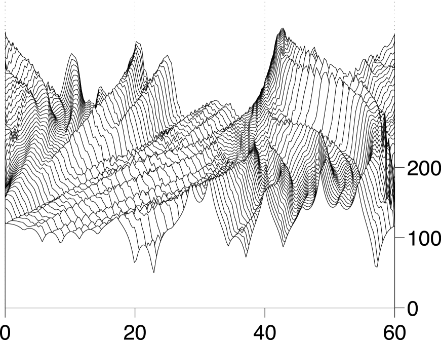
Figure 1. Numerical simulation demonstrates the evolution of an initial set of $\delta$-functions in $f$. The vertical coordinate represents $\overline{f}=H*f$, which remains finite even when $f$ forms $\delta$-functions for our choice $H(x)=e^{-|x|}$. This simulation of the initial value problem for equation (7.1) uses generalized initial conditions $f(x,0)=\sum_{a}p_{a}(0)\delta(x-q_{a}(0))$ with random initial amplitudes $-1/2<p_{a}(0)<1/2$.

We assume initial conditions for the scalar $f$ as

$$f(x,0)=p_{0}\delta(x-q_{0})+s\,p_{0}\delta(x-q_{0})\,.$$

Here, the sign $s=+1$ specifies symmetric initial conditions, whereas $s=-1$ enforces antisymmetric initial conditions. We shall choose the sign $s$ so the evolution due to (8.4,8.5) preserves the symmetric position of the $\delta$-function at $x=\pm q(t)$. If this choice is possible, then a solution of $p(t),q(t)$ in terms of quadratures can be found. Not all energies $E[f]$ and mobilities $\mu[f]$ allow symmetry preservation; however, many physically relevant cases do have this property. By reflection symmetry of the PDE, the even and odd parts of the solution are separately invariant. Consequently, we may assume a solution for all $t$ in the form,

(8.6) $$f(x,t)=p(t)\Big{(}\delta\left(x-q(t)\right)+s\,\delta\left(x+q(t)\right)\Big{)}\,.$$

Hence, the four equations (8.4,8.5) reduce by reflection symmetry to only two equations for $p(t),q(t)$:

(8.7) $$\dot{p}(t) = p(t)\,{\rm div}\,\Big{(}\frac{\delta E}{\delta f}\nabla\mu[f]\Big{)}^{\sharp}\bigg{|}_{x=\pm q(t)}$$

(8.8) $$\dot{q}(t) = \Big{(}\frac{\delta E}{\delta f}\nabla\mu[f]\Big{)}^{\sharp}\bigg{|}_{x=q_{a}(t)}$$

Let us first notice that the derivative is taken at $x=\pm q$, then

$$\,{\rm div}\,\Big{(}\frac{\delta E}{\delta f}\nabla\mu[f]\Big{)}^{\sharp}\bigg{|}_{x=\pm q(t)}=2\frac{\partial}{\partial q}\left(\Big{(}\frac{\delta E}{\delta f}\nabla\mu[f]\Big{)}^{\sharp}\bigg{|}_{x=\pm q(t)}\right)$$

If we now denote

(8.9) $$\Psi(p,q)=\left(\Big{(}\frac{\delta E}{\delta f}\nabla\mu[f]\Big{)}^{\sharp}\bigg{|}_{x=\pm q(t)}\right),$$

then equations (8.7,8.8) can be written as

(8.10) $$\dot{p}=2p\frac{\partial}{\partial q}\Psi(p,q)\,,\hskip 28.45274pt\dot{q}=\Psi(p,q)\,.$$

We are now ready to prove the following.

Theorem 2
Suppose $\Psi(p,q)$ defined by (8.9) is homogeneous with $\Psi(p,q)=p^{\gamma}\psi(q)$, and $s$ (symmetry parameter) is chosen so the solution retains its symmetry under the evolution. Then, a set of initial conditions $f=p_{0}\left(\delta(x-q_{0})+s\delta(x+q_{0})\right)$ exists, such that $q(t)$ in the solution (8.6) collapses $q\to 0$ in finite time, whenever $\psi(q)$ is a continuous function bounded away from zero with $|\psi(q)|\geq A>0$ in some neighborhood of $q=0$.
Note. Many physical choices of energy and mobility admit the required homogeneity of $\Psi(p,q)$. For example [7, 8] selected $\delta E/\delta f=G*f$, $\mu=1-H*f$, where $G$ and $H$ are given functions. This choice of energy and mobility implies $\Psi(p,q)=p^{2}\psi(q)$, so $\gamma=2$. Another example we shall employ here is $G(x)=e^{-x^{2}/\alpha^{2}}$ with $\alpha$ being a fixed parameter, and $\nabla\mu=1$, since the explicit formulas are particularly simple. This choice yields $\gamma=1$.
Proof of Theorem 2
First, let us notice that equations (8.10) integrate exactly (in terms of quadratures) if we assume that $\Psi(p,q)=p^{\gamma}\psi(q)$. Indeed, (8.10) are equivalent to

(8.11) $$\frac{dp}{dq}=2p\frac{1}{\psi(q)}\frac{d}{dq}\psi(q)$$

which integrates exactly in terms of initial conditions $p(0)=p_{0}$, $q(0)=q_{0}$ as

$$p=p_{0}\left(\frac{\psi(q)}{\psi(q_{0})}\right)^{2}.$$

Notice that by the assumption $|\psi(q)|\geq A>0$ in some neighborhood of $q=0$ we can choose $q_{0}$ sufficiently close to $0$ so $\psi(q_{0})\neq 0$. Then, the $q$-equation of (8.10) gives

(8.12) $$\dot{q}=p_{0}\psi(q_{0})^{-2\gamma}\psi(q)^{2\gamma+1}$$

If, by assumption, $\psi(q)<-A<0$ if $|q|<\delta$ for some $A>0,\delta>0$, let us choose $p_{0}>0$ and $0<q_{0}<\delta$. Then

$$\dot{q}\leq-\frac{p_{0}}{\psi(q_{0})^{-2\gamma}}A^{2\gamma+1}$$

so $q(t)$ goes to zero in time $t_{*}$ not exceeding

(8.13) $$t_{*}\leq\frac{q_{0}\psi(q_{0})^{2\gamma}}{p_{0}A^{2\gamma+1}}$$

The case $\psi(q)\geq A>0$ is treated analogously by choosing $p_{0}<0$.
We performed a simulation of the evolution of a scalar with initial conditions of the type (8.1). More precisely, we chose $\delta E/\delta f=G*f$ with $G(x)=e^{-x^{2}\alpha^{2}}$, and $\nabla\mu=1$. This gave values $\gamma=1$, $\psi(q)=e^{-4q^{2}/\alpha^{2}}$, so $\psi$ satisfies the conditions of the theorem. We chose initial conditions $f=p_{0}(\delta(x-q_{0})-\delta(x+q_{0}))$, since in this case, the antisymmetric solutions preserve symmetry under evolution, with the choice $p_{0}=-1/8$, $q_{0}=5/3$.

The evolution of positions for $\delta$-functions for this simulation is shown in Figure 2. The exact solution is shown with a solid line. The dashed line illustrates the position according to the numerics. The exact solution collapses in finite time whereas the numerical solution shows exponentially slow approach of the $\delta$-peaks. We attribute the apparent discrepancy for large time to numerical dissipation. Indeed, introducing a term $-\epsilon p$ mimicking numerical dissipation in the right-hand side of the $p$ equation in (8.10) prevents solution collapse, for any $\epsilon>0$, however small $\epsilon$ may be. Since every numerical scheme must necessarily involve some numerical dissipation or distortion, we believe it may be difficult to construct a numerical scheme that shows exact collapse of the solutions. This numerical question will be addressed elsewhere in future studies.

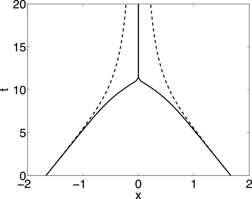
Figure 2. Collapse of a solution with initial condition having two $\delta$-functions with equal strength, opposite in sign $f(x,0)=p_{0}\left(\delta(x-q_{0})-\delta(x+q_{0})\right)$ with $p_{0}=1/8$, $q_{0}=2$. Exact solution is shown with a solid line, results of numerics is given with a dashed line.

The solution behavior may be investigated further by comparing the numerical and exact solutions for amplitude (8.4) in the evolution of a single $\delta$-peak. For this comparison, one may start with a single delta-function $f(x,0)=p_{0}\delta(x)$ and choose parameters $\mu=1-H*f$, $\delta E/\delta f=G*f$ and $G(x)=e{-|x|}$, $H(x)=\frac{1}{2}e^{-|x|}$. In this case, equation (8.4) reduces to $\dot{p}=-2p^{3}$, whose solution is

(8.14) $$\frac{1}{p^{2}}=\frac{1}{p_{0}^{2}}+4t$$

We illustrate the validity of this prediction in Fig. 3.

Figure 3. Evolution of the $1/p(t)^{2}$ versus time (circles). The theoretical prediction (8.14) is shown as a solid line. Note that (8.14) contains no fitting parameters.

The equations for the singular-solution parameters $\,p_{a}$ and $\boldsymbol{q}_{a}$ for the other quantities in equation (8.3) may be found the same way, by substituting the solution ansatz (8.3) above into the formulas (2.17,5.1,8.2) and matching terms.

Not unexpectedly, the density case recovers previous results for the HP equation.

9. $so(2)$- and $so(3)$-valued densities and gyrons

9.1. Derivation of equations

An interesting situation for practical applications occurs in the evolution of particles whose mutual interaction depends on their relative orientation. One example familiar from everyday life is the attraction of floating particles of non-circular shape, such as squares or stars. In this situation, the attraction between any two particles arising through their mutual deformation of the surface depends on their relative orientation.

Let us consider the motion of a set of particles whose energy $E$ depends on their relative orientations. A reasonable physical assumption is that each particle carries its own measure of orientation. (This is the case with floating particles – stars and squares, say.) However, notice that the rotation angle and density are independent – one may find dense regions with little relative rotation and regions of small mass density but large relative rotation. This possibility leads us to study the evolution of a physical quantity $\kappa$ which carries mass density and orientation separately. Mathematically, this corresponds to a density (an element of $\Lambda^{3}$) that carries a “charge” taking values in the real numbers $\mathbb{R}$ for the mass and in the dual of the Lie algebra $so(n)^{*}$ with $n=2$ or $3$ for orientation in two or three dimensions. Such a quantity is written as $\kappa\in(\mathbb{R}\otimes so(n)^{*})\otimes\Lambda^{3}$. These are (dual) Lie-algebra-valued “charge” densities. Let $e_{a}$ with $a=1,2,\dots,n(n-1)/2$ be a set of basis vectors for the Lie algebra $so(n)$. These basis vectors satisfy

(9.1) $$\left[e_{b},e_{c}\right]=t^{d}_{bc}e_{d}\hskip 28.45274pt(b,c,d>0)\,,$$

and $t^{d}_{bc}$ are the structure constants of the Lie algebra $so(n)$. For the case $n=3$ one recovers the familiar result that $t^{d}_{bc}=\epsilon_{ab}^{c}$ is the completely antisymmetric tensor density. Let us expand $\kappa$ in terms of the dual basis elements $e^{a}$ satisfying $\langle\,e_{a}\,,\,e^{b}\,\rangle=\delta^{b}_{a}$ in the form

(9.2) $$\kappa\,\mbox{d}^{n}x=\kappa_{a}e^{a}\mbox{d}^{n}x\,.$$

Here, the summation on the Lie algebra index $a$ ranges from $zero$ (for the mass density) to $dim(so(n))=n(n-1)/2$ for the orientation degrees of freedom. Thus, $a=0$ corresponds to the real-valued mass density and $a=1,2,\dots,n(n-1)/2$ denote the basis vectors of $so(n)$.

The Lie algebra $so(3)$ has three basis vectors. In contrast, $so(2)$ has only one basis vector, since only one number – angle of rotation – is sufficient to describe the rotation in two dimensions. Then, for example, in three dimensions we have $\kappa\in(\mathbb{R}\otimes so(3)^{*})\otimes\Lambda^{3}$. Correspondingly, the energy variation is given by $\delta E/\delta\kappa\in\mathbb{R}\otimes so(3)$ and is a function that takes real values for $a=0$ and takes values in the Lie algebra for $a>0$. The distinction between $so(3)$ and its dual $so(3)^{*}$ is purely notational for the present case, since these may both be identified with $\mathbb{R}^{3}$. However, we shall write the formulas below in notation that would be valid for an arbitrary Lie algebra.

The evolution equation for $\kappa\in(\mathbb{R}\otimes so(3)^{*})\otimes\Lambda^{3}$ in the space of densities taking values in the dual Lie algebra $so(3)^{*}$ is expressed as a pairing with a Lie algebra valued function $\phi\in\Lambda^{0}\otimes so(3)$. The mobility $\mu\in(\mathbb{R}\otimes so(3)^{*})\otimes\Lambda^{3}$ lies in the same space as $\kappa$. Let us introduce the real-valued velocity vector $\boldsymbol{\eta}=-\kappa_{b}\mathbf{D}^{\sharp}\phi^{b}$, where the spatial covariant derivative operator $\mathbf{D}$ is expressed in components as,

(9.3) $$D_{j}=\partial_{j}+{\rm ad}^{*}_{A_{j}}\,,\quad\hbox{or}\quad(D_{j}\phi)^{d}=(\delta^{d}_{a}\partial_{j}+t^{d}_{ab}A_{j}^{b})\phi^{a}\,.$$

Here, one sums over Lie algebra index $b$ and the operation $(\,\cdot\,)^{\sharp}$ in $\boldsymbol{\eta}=-\kappa_{b}\mathbf{D}^{\sharp}\phi^{b}$ raises the spatial index. This vector field has components

(9.4) $$\eta^{j}=-\kappa_{b}(D^{j}\phi)^{b}:=-\,\kappa_{b}\Big{(}\frac{\partial}{\partial x^{j}}\phi^{b}\Big{)}^{\sharp}+\kappa_{a}t_{cb}^{a}A^{jc}\phi^{b}\,.$$

Thus, $\boldsymbol{\eta}$ is a real vector field in $\mathbb{R}^{n}$. This formula expresses Darcy law velocity for Lie-algebra-valued quantities by using the spatial derivative in covariant form, with Lie-algebra-valued connection $\mathbf{A}^{c}e_{c}$ whose $j-$th spatial component is ${A_{j}}^{c}e_{c}$, with $j=1,2,\dots,n$ and $({A_{j}}^{c}e_{c})^{\sharp}=A^{jc}e_{c}$.

Likewise, we introduce the covariant time evolution operator as,

(9.5) $$D^{*}_{t}\kappa=\partial_{t}\kappa+{\rm ad}^{*}_{A_{0}}\kappa=(\partial_{t}\kappa_{a}+t^{d}_{ab}A^{b}_{0}\kappa_{d})e^{a}\,,$$

where $A_{0}=A^{a}_{0}e_{a}\in so(3)$ is the temporal component of the Lie algebra valued connection. We also introduce the covariant spatial divergence, cf. equation (9.3), as

(9.6) $$\mbox{Div}^{*}\kappa\boldsymbol{\eta}=D_{j}(\kappa\eta^{j})=\partial_{j}(\kappa\eta^{j})+{\rm ad}^{*}_{A_{j}}\kappa\eta^{j}\,.$$

Finally, we are ready to compute the covariant evolution equation. Applying the previous definitions and integrating by parts yields

$$\left<{\rm D}_{t}^{*}\kappa\,,\,\phi\right> = \left<\delta\kappa,\,\frac{\delta E}{\delta\kappa}\right>:=\left<-\,{\rm Div}^{*}\mu[\kappa]\boldsymbol{\eta},\,\frac{\delta E}{\delta\kappa}\right>=\left<\mu[\kappa]\boldsymbol{\eta},\,\mathbf{D}\,\frac{\delta E}{\delta\kappa}\right>$$

$$= \left<\mu[\kappa](-\kappa_{b}\mathbf{D}^{\sharp}\phi^{b}),\,\mathbf{D}\,\frac{\delta E}{\delta\kappa}\right>=\left<{\rm Div}^{*}\left(\kappa\Big{(}\mu[\kappa]_{a}\mathbf{D}^{\sharp}\frac{\delta E}{\delta\kappa_{a}}\Big{)}\right),\,\phi\right>\,.$$

Thus, we find the same equation we would have derived from thermodynamics, now written in terms of Lie-algebraic covariant derivatives,

(9.7) $${\rm D}_{t}^{*}\kappa={\rm Div}^{*}\left(\kappa\Big{(}\mu[\kappa]_{a}\mathbf{D}^{\sharp}\frac{\delta E}{\delta\kappa_{a}}\Big{)}\right)\,.$$

As one might have expected, this is the covariant form of the HP equation (7.4) for the orientation “charge density” $\kappa=\kappa_{b}e^{b}$ taking values in the dual of the Lie algebra. This is the covariant evolution equation we sought for interaction energies that depend on both particle densities and orientations.

The covariant form of Lie-algebra-valued scalar GOP equation. Comparing the patterns of equations (7.4) and (9.7) with that for the scalar case (7.1), we may immediately write the corresponding dynamics for a Lie-algebra-valued scalar $f=f^{a}e_{a}$ in covariant form, as

(9.8) $$D_{t}f = -\,\Big{(}\frac{\delta E}{\delta f}\,\mathbf{D}\mu[f]\Big{)}^{\sharp}\cdot\mathbf{D}f\,.$$

The index notation for the spatial and temporal covariant derivatives of densities in the dual Lie algebra was explained, respectively, in equations (9.3) and (9.5). The scalar equation (9.8) may also be expressed in index notation by raising or lowering the Lie algebra indices appropriately. This observation also sets the pattern for generalizing other GOP flows to Lie-algebra values.

Particular modeling choices for $SO(3)$. The Lie-algebra-valued connections $A_{0}$ and $\mathbf{A}$ are not yet defined. One may identify a good candidate for $A_{0}$ by examining the limit when the mobility vanishes, $\mu[\kappa]=0$. In this limit, when we choose the Lie algebra $so(3)$, and make a particular choice of $A_{0}$, equation (9.7) reduces to the famous Landau-Lifshitz equation for spin waves,

(9.9) $${\rm D}_{t}^{*}\kappa=(\partial_{t}\kappa_{a}-\epsilon^{d}_{ab}A^{b}_{0}\kappa_{d})e^{a}=0\,,$$

or, in obvious vector notation,

(9.10) $$\partial_{t}\kappa-A_{0}\times\kappa=0\,.$$

The Landau-Lifshitz equation now emerges upon making the choice $A_{0}={\delta E/\delta\kappa}$, so that

(9.11) $$\partial_{t}\kappa=\frac{\delta E}{\delta\kappa}\times\kappa=\kappa\times\Delta\kappa\,,\quad\hbox{when}\quad\frac{\delta E}{\delta\kappa}=-\,\Delta\kappa\,.$$

It remains to choose the spatial connection $\mathbf{A}$ as our final modeling parameter. For the sake of simplicity, in the rest of the paper we shall make the choice,

$$\mathbf{A}\cdot\mbox{d}\mathbf{x}=d\chi\chi^{-1}\in so(3)$$

with $\chi$ in the order parameter group $SO(3)$. This choice is a “pure gauge” connection whose spatial curvature is always zero. The quantity $\chi\in SO(3)$ is an auxiliary variable defined by relating its advective time derivative to the temporal part of the connection $A_{0}$ as

$$\dot{\chi}:=\frac{\partial\chi}{\partial t}+\mathbf{u}\cdot\nabla\chi=A_{0}\chi\quad\hbox{where}\quad\mathbf{u}=\Big{(}\kappa\diamond\frac{\delta E}{\delta\kappa}\Big{)}^{\sharp}\quad\hbox{and}\quad A_{0}=\frac{\delta E}{\delta\kappa}\,.$$

From its definition, one finds an evolution equation for the spatial part of the connection form,

(9.12) $$(d\chi\,\chi^{-1})\dot{\,}=(\mathbf{A}\cdot\mbox{d}\mathbf{x})\dot{\,} = \big{(}\partial_{t}\mathbf{A}+\mathbf{u}\cdot\nabla\mathbf{A}+(\nabla\mathbf{u)^{T}}\cdot\mathbf{A}\big{)}\cdot\mbox{d}\mathbf{x}$$

$$= dA_{0}+{\rm ad}_{A_{0}}(\mathbf{A}\cdot\mbox{d}\mathbf{x})$$

$$= \big{(}\partial_{j}A_{0}^{a}+\epsilon^{a}_{bc}A_{0}^{b}{A}_{j}^{c}\big{)}e_{a}\mbox{d}x^{j}$$

where $A_{0}=A^{b}_{0}e_{b}\in so(3)$ is the temporal component of the Lie algebra valued connection. This formula closes the system. Given the choice $A_{0}={\delta E/\delta\kappa}$ and the relation $A_{0}=\dot{\chi}\chi^{-1}$ for the auxiliary variable $\chi$, this calculation of the evolution equation for $\mathbf{A}\cdot\mbox{d}\mathbf{x}=d\chi\chi^{-1}$ extends to any order parameter group. The resulting system is

(9.13) $${\rm D}_{t}^{*}\kappa = {\rm Div}^{*}\left(\mu[\overline{\kappa}]\Big{(}\kappa_{a}\mathbf{D}^{\sharp}\frac{\delta E}{\delta\kappa_{a}}\Big{)}\right)$$

(9.14) $$\partial_{t}\mathbf{A} + \mathbf{u}\cdot\nabla\mathbf{A}+(\nabla\mathbf{u)^{T}}\cdot\mathbf{A}=\nabla A_{0}+{\rm ad}_{A_{0}}\mathbf{A}$$

where $\mathbf{u}=\Big{(}\kappa\diamond\frac{\delta E}{\delta\kappa}\Big{)}^{\sharp}$ and $A_{0}=\frac{\delta E}{\delta\kappa}$. In general, if the connection terms are small compared to spatial gradients, (9.14) becomes simply a nonlinear diffusion equation. Alternatively, if the connection terms are much larger than the spatial gradients, right-hand side of (9.14) becomes an integrable double-bracket equation considered in [24]). The left hand side of (9.14) drives the evolution of $\kappa$ through the presence of time derivative and Landau-Lifshitz terms.

9.2. Measure-valued solutions: gyrons

A special case that warrants further investigation arises when the Lie algebra in question is abelian, so that the structure constants vanish. As we shall show below, this case yields singular solutions.

Let us multiply (9.7) by an arbitrary function $\phi\in\mathbb{R}\otimes so(3)$. After the first integration by parts, we find

(9.15) $$\left<\frac{\partial\kappa_{b}}{\partial t},\phi^{b}\right>=\left<\kappa_{b}\bigg{(}\mu[\kappa]_{a}\frac{\partial}{\partial x^{j}}\frac{\delta E}{\delta\kappa_{a}}\bigg{)}^{\sharp},\,\frac{\partial\phi^{b}}{\partial x_{j}}\right>\,.$$

By proceeding analogously to the calculation of HP clumpons in previous sections, we see that singular solutions of the form

(9.16) $$\kappa_{a}=\int p_{a}(s,t)\delta(\mathbf{x}-\mathbf{q}(s,t))\mbox{d}s$$

are admitted, in which $p_{a}$ takes values in the dual Lie algebra. Since the right hand side of (9.15) contains no terms proportional to $\phi^{a}$, we find that $\partial_{t}p_{a}(s,t)=0$, for $a=0,1,\ldots,dim(so(n))$. Equations for the $j$-th component of $\mathbf{q}$ which are expressed from the equation for component $b$ are:

(9.17) $$p_{b}\frac{\partial q^{j}}{\partial t}=p_{b}\bigg{(}\mu[\kappa]_{a}\rm{D}_{j}\frac{\delta E}{\delta\kappa_{a}}\Big{|}_{(\mathbf{x}=\mathbf{q})}\bigg{)}^{\sharp}.$$

Assuming that $p_{b}\neq 0$, we get simple evolution equations for the strength $p$ and coordinates $q_{j}$:

(9.18) $$\frac{\partial p_{a}}{\partial t}=0\hskip 28.45274pt\frac{\partial q^{j}}{\partial t}=\bigg{(}\mu[\kappa]_{a}\rm{D}_{j}\frac{\delta E}{\delta\kappa_{a}}\Big{|}_{(\mathbf{x}=\mathbf{q})}\bigg{)}^{\sharp}.$$

As we shall see, the singular solutions (gyrons) do appear in experiments. Thus, the singular solutions derived here are an essential part of the dynamics for particles with orientation.

9.3. Comparison with experiments for the case of floating five-point stars

illustrate the power of our theory and connect it with the original problem of self-assembly of particles with orientation, we present a numerical simulation of the system (9.14) formulated for the particular case of a five-point floating stars.

In order to formulate (9.14) explicitly, we must first find a suitable approximation for the energy as a functional of density and orientation. Denote the density at a point $\boldsymbol{x}$ as $\rho(\boldsymbol{x})$ and orientation as $\sigma(\boldsymbol{x})$. If the energy between particles due to density is given by the (half)-sum of binary interactions (which is a suitable approximation for dilute states), the ’density’ part of the energy gives

(9.19) $$E_{\rho}=\frac{1}{2}\int\rho(\boldsymbol{x})\rho(\boldsymbol{x}^{\prime})G(\boldsymbol{x}-\boldsymbol{x}^{\prime})\mbox{d}\boldsymbol{x}\mbox{d}\boldsymbol{x}^{\prime}$$

For a given $\sigma(\boldsymbol{x})$, the orientation represents a vector with cartesian coordinates $(\cos\sigma(\boldsymbol{x}),\sin\sigma(\boldsymbol{x}))$. If we assume that a function $\boldsymbol{H}\left(\sigma(\boldsymbol{x}),\sigma(bx^{\prime})\right)$ describes interaction of orientations, then the energy due to orientations is given by

(9.20) $$E_{\sigma}=\frac{1}{2}\int\rho(\boldsymbol{x})\rho(\boldsymbol{x}^{\prime})\boldsymbol{H}\left(\sigma(\boldsymbol{x}),\sigma(\boldsymbol{x}^{\prime})\right)\mbox{d}\boldsymbol{x}\mbox{d}\boldsymbol{x}^{\prime}$$

One possible approximation would be to assume that the interaction function $\boldsymbol{K}$ is simply proportional to the scalar product between $\sigma(\boldsymbol{x})$ and $\sigma(\boldsymbol{x}^{\prime})$. However, for the case of interacting stars or any objects with an $m$-fold symmetry, we must take into account that $\sigma(\boldsymbol{x})$ and $\sigma(\boldsymbol{x}^{\prime})$ can differ by $2\pi/m$ without affecting the interaction energy. Thus, the following form of the interaction energy is proposed:

(9.21) $$E_{\sigma}=\frac{1}{2}\int\rho(\boldsymbol{x})\rho(\boldsymbol{x}^{\prime})K\big{(}|\boldsymbol{x}-\boldsymbol{x}^{\prime}|\big{)}\cos\left[m\big{(}\sigma(\boldsymbol{x})-\sigma(\boldsymbol{x}^{\prime})\big{)}\right]\mbox{d}\boldsymbol{x}\mbox{d}\boldsymbol{x}^{\prime}$$

Here, $K(r)$ is a scalar smoothing function, which must be determined from physical reasoning. An interesting case relevant for the evolution of the ‘pointy’ objects is that the orientation part of the energy $E_{\sigma}$ is of much longer range than the density part $E_{\rho}$. The total energy is then simply

(9.22) $$E[\kappa]=E_{\rho}+E_{\sigma},$$

where $\kappa=(\rho,\sigma)$.

In Figure 4 we present a numerical simulation for the evolution in two dimensions of a collection of five-point stars ($m=5$). In this case, there are two unknown variables: the mass density $\rho$, which multiplies the basis vector of $e_{0}$, and orientation $\sigma$ which is the coefficient of the basis vector $e_{1}$. The initial conditions for the evolution are taken to be a gaussian distribution of initial density, possessing random initial orientations (Fig. 4, top left). In the simulation, we observe the formation of large-scale structures which are predominantly either individual line segments or arrangements of three line segments meeting at a point to form a star-like structure (Fig. 4, top right). An experiment, conducted by P. D. Weidman, started with 4mm plastic floating stars distributed within a circular shape with random initial orientation (Fig. 4, bottom left). The stars are positioned on a net which is lowered slowly into the fluid. Care is taken to avoid residual water motion and convection. After 1 hour, the stars were found to assemble into line shapes or several-armed structures. Three-armed structures seem to be most common (Fig. 4, bottom right). While the position of the large-scale formations in the experiment is random and therefore impossible to predict analytically, the predominant shapes found in the experiment are reproduced in simulations using our model.

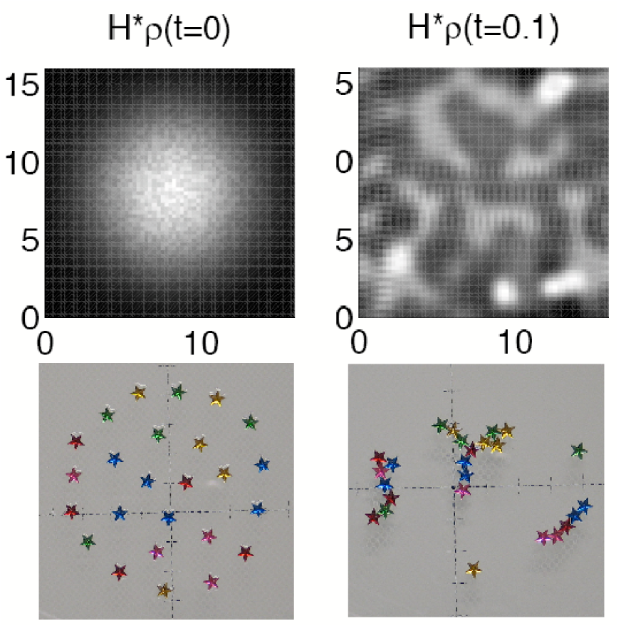
Figure 4. Top: Numerical simulation of density $\overline{\rho}=H*\rho$ where $H(\mathbf{r})=e^{-\mathbf{r}^{2}}$ is a Gaussian filter. White denotes the areas with high density whereas black marks the areas with small density. Left: initial state for density, taken to be Gaussian:$\rho(\mathbf{r},0)=\rho_{0,k}e^{-|\mathbf{r}|^{2}/l_{\rho}^{2}}$. In the simulation, the particles are assumed to have a five-fold symmetry. The initial conditions for orientation are random. Top right: final state. Bottom: an experiment reproducing this numerical solution (courtesy of P.D.Weidman). Bottom left: initial conditions - five-point stars are positioned on a net and slowly lowered into the fluid. Initial orientations for the stars are random. Bottom right: final state after 1 hr.

10. Acknowledgements

We are indebted to Cesare Tronci for his insightful comment about a key step in the derivation of the GOP equation, that made the diamond-form of Darcy’s law more generally applicable. This improvement will be pursued elsewhere. We are grateful for stimulating discussions with P. D. Weidman, whose remarkable experiments on anisotropic floating particles set this work in motion. We are also grateful for the permission to use Prof. Weidman’s experimental results in this work. We are also grateful to S. R. J. Brueck, who introduced us to the fascinating world of nanoscale self assembly. The authors were partially supported by NSF grant NSF-DMS-05377891. The work of DDH was partially supported by the Royal Society of London and the US Department of Energy Office of Science Applied Mathematical Research. VP acknowledges the support of von Humboldt foundation and the hospitality of the Institute for Theoretical Physics, University of Köln where this work was completed.

References

- [1] B. A. Grzybowski, G. M. Whitesides, Self-Assembly at All Scales Science, 295, 2418 (2002).
- [2] E. Rabani et al. D. R.Reichman, P. L.Geissler and L. E.Brus, Drying mediated self-assembly of nano-particles, Nature, 426, 271 (2003).
- [3] D. Xia and S. Brueck, A Facile Approach to Directed Assembly of Patterns of Nanoparticles Using Interference Lithography and Spin Coating, Nano Lett., 4, 1295(2004).
- [4] N. Bowden I. S. Choi, B. A. Grzybowski and G. M. Whitesides, Mesoscale self-assembly of hexagonal plates using lateral capillary forces: Synthesis using the capillary bond J. Am. Chem. Soc. 121, 5373 (1999).
- [5] B. A. Grzybowski et al. , N. Bowden, F. Arias, H. Yang and G. M. Whitesides, Modeling of Menisci and Capillary Forces from the Millimeter to the Micrometer Size Range J.Phys.Chem.B 105, 404 (2001).
- [6] B. A. Grzybowski, C. J. Campbell Chem.Eng.Sci 59,1667 (2004).
- [7] D. D. Holm and V. Putkaradze, Aggregation of finite-size particles with variable mobility Phys Rev Lett, 95, 226105 (2005).
- [8] D. D. Holm and V. Putkaradze, Formation of clumps and patches in self-aggregation of finite size particles Physica D, to appear; ArXiv:nlin.PS/0506020 (2006).
- [9] M. V. Smoluchowski, Versuch einer mathematischen Theorie der Koagulationskinetik kolloider Lösungen. Z. Phys. Chem. 92, 129-168 (1917). USA. 95:9280-9283.
- [10] P. Debye and E. Hückel, Zur Theorie der Elektrolyte: (2): Das Grenzgesetz für die Elektrische Leiftfahrigkeit (On the theory of electrolytes 2: limiting law of electrical conductivity). Phys. Z. 24, 305 (1923).
- [11] E. F. Keller and L. A. Segel, Initiation of slime mold aggregation viewed as aninstability. J. Theo. Biol. 26, 399 (1970); Ibid. Model for chemotaxis. J. Theo. Biol. 30, 225 (1971).
- [12] D. Horstmann, From 1970 until present: the Keller-Segel model in chemotaxis and its consequences. MPI Leipzig Report (2003).
- [13] C. M. Topaz, A. L. Bertozzi and M. A. Lewis, A nonlocal continuum model for biological aggregation Bull. Math. Bio. (2006), to appear, ArXiv: q-bio PE/0504001 (2005).
- [14] P. H. Chavanis, C. Rosier and C. Sire, Thermodynamics of self-gravitating systems, Phys.Rev. E 66 036105 (2002).
- [15] J.D. Gibbon and E.S. Titi, Cluster formation in complex multi-scale systems, Proc. Royal Soc. London Ser. A, 461, 3089 (2005).
- [16] R. Camassa, D D Holm An integrable shallow water equation with peaked solitons. Phys. Rev. Lett. 71, 1661 (1993).
- [17] D.D. Holm, J.E. Marsden and T.S. Ratiu, The Euler–Poincaré equations and semidirect products with applications to continuum theories. Adv. in Math., 137, 1-81 (1998). http://xxx.lanl.gov/abs/chao-dyn/9801015.
- [18] D.D. Holm and J.E. Marsden, Momentum maps and measure valued solutions (peakons, filaments, and sheets) of the Euler-Poincar e equations for the diffeomorphism group. In The Breadth of Symplectic and Poisson Geometry, A Festshrift for Alan Weinstein, 203-235, Progr. Math., 232, J.E. Marsden and T.S. Ratiu, Editors, Birkhäuser Boston, Boston, MA, 2004. http://arxiv.org/abs/nlin.CD/0312048
- [19] F. Otto, The geometry of dissipative evolution equations: the porous medium equation. Comm. Partial Diff. Eqs. 26, 101–174 (2001).
- [20] V.E. Zakharov, V.S. L’vov, S.S Starobinets Turbulence of spin-waves beyond threshold of their parametric-excitation, Usp. Fiz. Nauk 114, 4 (1974), 609–654; English translation Sov. Phys. - Usp. 17, 6 (1975), 896–919.
- [21] J.J.L. Velazquez, Stability of Some Mechanisms of Chemotactic Aggregation SIAM J. Appl. Math, 62, 1581 (2002).
- [22] J. P. Ortega, V. Planas-Bielsa, Dynamics on Leibnitz Manifolds, J. of Geometry and Physics, 52, 1-27 (2004); arXiv:math.DS/0309263.
- [23] P.G. Saffman, Vortex Dynamics. CUP Cambridge (1992).
- [24] A. M. Bloch, R. W. Brockett and T.S.Ratiu, Completely integrable gradient flows, Comm. Math. Phys. 147, 57-74 (1992).
- [25]