Geometry of intensive scalar dissipation events in turbulence

Abstract

Maxima of the scalar dissipation rate in turbulence appear in form of sheets and correspond to the potentially most intensive scalar mixing events. Their cross-section extension determines a locally varying diffusion scale of the mixing process and extends the classical Batchelor picture of one mean diffusion scale. The distribution of the local diffusion scales is analysed for different Reynolds and Schmidt numbers with a fast multiscale technique applied to very high-resolution simulation data. The scales take always values across the whole Batchelor range and beyond. Furthermore, their distribution is traced back to the distribution of the contractive short-time Lyapunov exponent of the flow.

When a scalar concentration field $\theta({\bf x},t)$ is transported in a turbulent flow very large scalar gradients are generated which can be associated with potentially intensive mixing Dimotakis2005 . Frequently, such large-amplitude gradient regions exist across scales that are finer than the smallest turbulent eddies, a case which is known as the Batchelor regime of scalar mixing Batchelor1959 . Their cross-section is usually estimated by a single mean diffusion scale, the Batchelor scale $\eta_{B}$, that equilibrates advection by flow and scalar diffusion. However, scalar gradients are known to fluctuate strongly in turbulent mixing. These fluctuations are caused by the fluctuating scalar amplitudes and by the varying spatial sections across which the scalar differences are built up. Both aspects will cause the strong spatial variability of potentially intensive mixing regions. Thus, a whole range of local diffusion scales $l_{d}$, which quantifies exactly this variability, will exist around the mean diffusion scale $\eta_{B}$. Their distribution is interesting for several reasons. It can enter mixing efficiency measures Doering2004 . The scales prescribe the extension of chemically reactive layers in which the combustion of fuel takes place Peters2000 or the variations of the fluorescence signal as used for the measurement of zooplankton patchiness in the ocean Wolk .

In this Letter, we want to calculate this local diffusion scale distribution $p(l_{d})$. It arises from the competition of two dynamic processes. On one hand, the scale distribution will be affected by molecular diffusion that causes a diminishing of existing steep gradients as well as the completion of their formation by reconnection Gibson1968 ; Villermaux2003 . On the other hand, the scales will be determined by the statistics of the local advection flow patterns that pile up scalar differences. While the strongest scalar gradients were related to instantaneous velocity gradients in Ref. Schumacher2003 , we will go one step further in the second part of the Letter and relate the local diffusion scale distribution to the distribution of Lagrangian contraction rates of the flow, as given by the smallest of the three finite-time Lyapunov exponents along Lagrangian trajectories. The Lagrangian approach incorporates the temporal evolution of the persistent flow patterns that eventually generate the strongest scalar gradients or the finest local dissipation scales in a finite time. The analysis is conducted for passive scalars in Navier-Stokes turbulence, a case that is not accessible to analytical treatment. Our investigations are therefore based on direct numerical simulations (DNS). In order to discuss trends with Reynolds and Schmidt number, we analyze five different data sets. Very high-resolution calculations (with up to $1024^{3}$ grid points) have to be conducted with resolution constraints that exceed the usually applied ones such that the finest scales of the turbulent mixing process are resolved properly. The fluctuations of the flow are sustained statistically stationary by a large-scale random forcing and the passive scalar is driven by a constant mean scalar gradient. We consider the scalar dissipation field diss which probes the magnitude of scalar gradients and which is defined as

$$\epsilon_{\theta}({\bf x},t)=\kappa|{\bf\nabla}\theta({\bf x},t)|^{2}\,.$$ (1)

Here, $\kappa$ is the scalar diffusivity. Experimental studies on the geometry of scalar dissipation fields are very challenging since gradients have to be measured and only a few exist Buch1998 ; Su2003 .

Figure 1 shows a two-dimensional (2D) slice cut through a DNS snapshot of $\epsilon_{\theta}({\bf x},t)$. We observe strongly folded filaments. The points that form the level set of largest dissipation amplitudes

$$L_{C}=\{{\bf x}:\epsilon_{\theta}\geq C\langle\epsilon_{\theta}\rangle\;\mbox{or}\;|{\bf\nabla}\theta|\geq\sqrt{C\langle|\nabla\theta|^{2}\rangle}\}\,,$$ (2)

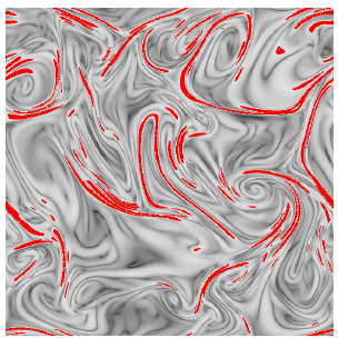
Figure 1: (color online) Contour plot of a two-dimensional slice cut through the instantaneous three-dimensional scalar dissipation rate field. Level set $L_{C}$ for $C=4$ (see Eq. (2)) is replotted in red. Data are from a pseudospectral simulation of the advection-diffusion equation for the passive scalar in combination with Navier-Stokes equations for a statistically stationary, homogeneous isotropic flow at a resolution of $1024^{3}$ grid points in a periodic box $V=(2\pi)^{3}$ Schumacher2003 . The Schmidt number is $Sc=\nu/\kappa=32$ and the Taylor microscale Reynolds number is $R_{\lambda}=\sqrt{15/(\nu\langle\epsilon\rangle)}\,\langle u_{x}^{2}\rangle=24$ with $\langle\epsilon\rangle$ being the mean energy dissipation rate and $\nu$ the kinematic viscosity. The Batchelor scale $\eta_{B}=\eta/\sqrt{Sc}$ is resolved with 2 grid cells. The viscous Kolmogorov length $\eta=\nu^{3/4}/\langle\epsilon\rangle^{1/4}$ measures then 11 grid cells. This spectral resolution is larger by a factor of 4 than the one usually adopted.

are redrawn in red. $C$ is a real constant. The resulting filaments are cross-sections of thin sheets in which the maxima of scalar dissipation are arranged in the three-dimensional volume Schumacher2003 . A closer inspection of Fig. 1 unravels various length and thickness scales of the filaments. The filaments are curved and tightly clustered in certain locations thus posing a challenge of separating each curved filament and computing its accurate variation scales.

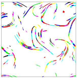
Figure 2: (color online) Reconstruction of the red colored filaments as shown in Fig. 1 by means of the fast multiscale clustering algorithm. Long filaments are composed of several subfilaments that are colored differently.

This is done here by a fast multiscale clustering algorithm Brandt2004 , which is based on the Segmentation by Weighted Aggregation (SWA) algorithm AMG , motivated by Algebraic Multigrid (AMG) SharonBrandtBasri2000 . The algorithm assigns data points into clusters starting at the finest resolution level, the grid spacing. All points ${\bf x}_{i}\in L_{C}$ are therefore gathered in a so-called proximity graph that contains their location and their connectivity to other points of $L_{C}$ as quantified by the inter-point weights which probe the nearest graph neighbors of each point only. Since the information about proximity is kept as one moves from finer to coarser resolution level, one can perform a fast recursive principal component analysis (PCA). The resulting eigenvalues characterize the length and width of the point clusters. Additionally, strongly curved filaments have to be decomposed into sub-filaments by applying a local convexity criterion along the filament. Figure 2 shows the reconstruction of the filaments from Fig. 1 and their division into sub-filaments. The local dissipation filament thickness, $l_{d}$, is then given by nothing else but the smaller eigenvalue which follows from the PCA of each sub-filament.

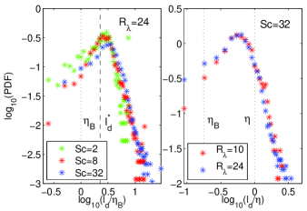
Figure 3: (color online) Distribution of the local cross-section thickness $l_{d}$ of the scalar dissipation rate filaments for $\epsilon_{\theta}\geq 4\langle\epsilon_{\theta}\rangle$. Left panel: Probability density function (PDF) $p(l_{d}/\eta_{B})$ for three different Schmidt numbers at $R_{\lambda}=24$. The dashed line corresponds with the theoretical value of the most probable scale $l_{d}^{*}=\sqrt{\kappa/|\Lambda_{3}|}$ which will be discussed later in the text. Right panel: PDF $p(l_{d}/\eta)$ for two different Reynolds numbers at $Sc=32$.

Figure 3 shows the probability density functions (PDF) of the local filament thickness $l_{d}$ for different Schmidt ($Sc$) and Reynolds numbers ($R_{\lambda}$). The distribution will depend on the cut-off level $C$, but the physical picture will not change since $C$ is fixed with respect to the mean scalar dissipation rate throughout the analysis. Local thickness values within the whole Batchelor range between $\eta_{B}$ and $\eta$ and beyond are found, indicating that dissipation maxima are also related to scalar gradients across inertial range scales. The 2D analysis does not account for the spatial orientation of the sheets with respect to the cutting plane. As demonstrated in Buch1998 , this will affect only the tail for large $l_{d}$. The left panel of Fig. 3 compares the PDFs for three different Schmidt numbers at a fixed Reynolds number $R_{\lambda}=24$. With increasing Schmidt number stronger jumps of the scalar concentration across finer thickness scales become more probable since diffusion is less dominant. Consequently, the most probable thickness $l_{max}$, i.e. the maximum of the distribution, is shifted to smaller values, but remains always larger than the corresponding Batchelor scale. This suggests that the formation of so-called mature scalar gradient fronts with a thickness $\sim\eta_{B}$ is a subdominant process. We see that the three PDFs overlap when rescaled with $\eta_{B}$ which implies that $l_{max}\sim Sc^{-1/2}$ on the basis of our data and even though $Sc=2$ has no real Batchelor range. In the right panel of Fig. 3, we compare distributions for two different Reynolds numbers at fixed Schmidt number. Both PDFs rescaled with the corresponding $\eta$ overlap again to a large fraction, except for the very fine scales. Their higher probability with increasing $R_{\lambda}$ indicates a more efficient stirring at the smallest scales. Our data show that the scale $l_{max}$ follows now the same dependence with Reynolds number as the Kolmogorov scale, i.e. $l_{max}\sim R_{\lambda}^{-3/2}$ This result is similar to finding in Buch1998 ; Su2003 for $Sc\sim 1$ and does not change for $Sc\gg 1$.

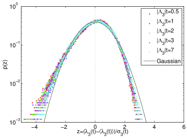
Figure 4: (color online) Probability density function of $\lambda_{3}(t)$ for different times. The data are for $R_{\lambda}=24$. The variable $z=(\lambda_{3}(t)-\langle\lambda_{3}(t)\rangle)/\sigma_{3}(t)$ with $\sigma_{3}(t)=\sqrt{\langle(\lambda_{3}(t)-\langle\lambda_{3}(t)\rangle)^{2}\rangle}$ is chosen for comparison with a Gaussian distribution. We found $\Lambda_{3}\simeq-0.425$ and $\sigma^{2}_{3}(t)=\sigma^{2}_{\infty}/t$ with $\sigma^{2}_{\infty}\simeq 0.44$ for $t\gtrsim|\Lambda_{3}|^{-1}$. The distribution is evaluated by $2.5\times 10^{5}$ Lagrangian tracers that are initially seeded uniformly. The distribution for $R_{\lambda}=10$ behaves qualitatively the same.

The filament thickness distribution is now related to the distribution of finite-time Lyapunov exponents (FTLE) $\lambda_{i}(t)$. They measure the local separation between two initially infinitesimally close fluid elements along the Lagrangian trajectory. Therefore an orthogonal frame is attached to each tracer and the three separation vectors evolve as $\mbox{d}\delta r_{j}^{(i)}(t)/\mbox{d}t=\sigma_{jk}(t)\,\delta r_{k}^{(i)}(t)$ for $j,k=x,y,z$ and $i=1,2,3$. $\sigma_{jk}(t)$ is the rate of strain tensor along the Lagrangian trajectories. The FTLEs follow to $\lambda_{i}(t)^{=}1/t\,\log(|\delta{\bf r}^{(i)}(t)|/|\delta{\bf r}^{(i)}(0)|)$ where the Gram-Schmid method is applied consecutively to three $\delta{\bf r}^{(i)}(t)$ (see Appendix C.3 of Bohr1998 ). The exponents will vary from trajectory to trajectory resulting in statistical distributions. Their means are the global FTLE, $\langle\lambda_{i}(t)\rangle$, which converge for long times to three numbers, the asymptotic Lyapunov exponents $\Lambda_{i}=\mbox{lim}_{t\to\infty}\langle\lambda_{i}(t)\rangle$. Due to incompressibility, $\sum_{i=1}^{3}\lambda_{i}(t)=0$. Our interest is in the formation of thin dissipation (or gradient) sheets where expansion in two directions is present, i.e. $\lambda_{1}(t)>0$ and $\lambda_{2}(t)>0$, and contraction in the third one, $\lambda_{3}(t)<0$. The distribution of contraction rates that pile up scalar gradient maxima and form the distribution of the local diffusion scales follows consequently from the PDF $p(\lambda_{3}(t))$ as shown in Fig. 4. We see that the cores of the distributions for different times collapse to a Gaussian profile within $\pm 2\sigma_{3}(t)$. Since the standard deviation $\sigma_{3}(t)=\sigma_{\infty}/\sqrt{t}$ for larger times the contraction rate $\lambda_{3}(t)$ will get more and more concentrated about $\Lambda_{3}$ as the time advances. Based on $\Lambda_{3}$ the most probable thickness is given as $l_{d}^{\ast}=\sqrt{\kappa/|\Lambda_{3}|}$ Balkovsky1999 which arises by equilibrating contractive strain and diffusion. For all data analysed this scale is at about the maximum of the thickness distribution, $l_{d}^{\ast}\simeq l_{max}$ (see left panel of Fig. 3).

Hu and Pierrehumbert Pierrehumbert2002 pointed out that the asymptotic $\Lambda_{3}$ alone is not sufficient to explain the formation of the finest diffusion scales when the flow is time-correlated as being the case for the present studies. The time that a scalar blob or filament experiences a persistent strain pattern along the trajectory can be estimated by a characteristic decorrelation time which is given by $\tau_{c}\sim\Lambda_{3}^{-1}$. For larger periods the persistent compression of the blob will disappear or the sheets undergo diffusive destruction or merging. This local scenario will appear repeatedly and causes a stationary thickness scale distribution. Consequently, we have to take into account the evolution of distribution of the FTLEs over such periods in order to study the formation of the gradient (or dissipation) sheets. The distribution of the sheets is related to the characteristic distribution of the FTLE over times $t\lesssim\tau_{c}$ by

$$p(l_{d}) \sim \int\mbox{d}l_{0}\,\tilde{p}(l_{0})\int_{-\infty}^{+\infty}\mbox{d}\lambda_{3}\,g(\lambda_{3})\,\delta\left(l_{d}-l_{0}\mbox{e}^{\lambda_{3}\tau_{c}}\right)$$ (3)

$$= \frac{1}{l_{d}\tau_{c}}\int\mbox{d}l_{0}\,\tilde{p}(l_{0})\,g(\log(l_{d}/\l_{0})/\tau_{c})\,,$$

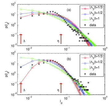
Figure 5: (color online) Distribution of the local cross-section thickness $l_{d}$ as reconstructed from the distribution of the FTLE $g(\lambda_{3})$ via Eq. (3) for different times. Data are for $R_{\lambda}=24$ and $Sc=32$ (see Fig. 3) . Two initial distributions are shown: (a) uniform distribution $\tilde{p}(l_{0})=1/(2\eta_{K}-\eta_{B})$; (b) delta function $\tilde{p}(l_{0})=\delta(l_{0}-1.8l_{d}^{*})$ (see Fig. 3). The grid spacing $\Delta$ and Kolmogorov scale $\eta$ are indicated as vertical arrows.

where the distribution of the FTLE is approximated by a Gaussian $g(\lambda_{3},t)=(1/\sqrt{2\pi\sigma_{3}(t)^{2}})\exp[-(\lambda_{3}(t)-\langle\lambda_{3}(t)\rangle)^{2}/(2\sigma_{3}(t)^{2})]$ and $\tilde{p}(l_{0})$ the (unknown) distribution of the initial thickness scales. The initial distributions $\tilde{p}(l_{0})$ taken here mark both ends of a spectrum of possible choices, the localized case given by a delta-function around the maximum of $p(l_{d})$ and a uniform distribution of initial scales over an interval, respectively. Both cases can be carried out analytically and result in scale distributions of log-normal type. Figure 5 shows the resulting PDFs for $R_{\lambda}=24$ and $Sc=32$. The distributions agree well with the data for most $l_{d}$ and for time periods $t\lesssim|\Lambda_{3}|^{-1}$. The uniform case fits slightly better for the left tail since sufficiently small scales are present initially that can be steepened further to smaller cross sections. The strain which is accumulated over short times only seems to explain the formation of the finest scalar gradient sheets. Nearly, the same time scales and distributions were found for the other Schmidt and Reynolds number values.

In conclusion, we have determined the distribution of the cross-section extensions of the scalar dissipation maxima in Navier-Stokes turbulence. These scales correspond with local diffusion scales and take values across the whole Batchelor range and beyond. By means of the distribution of smallest short-time Lyapunov exponent, the diffusion scale distribution can be reconstructed.

Acknowledgements. We acknowledge support by the NSF grant DMS-9810282 and thank the Institute for Pure and Applied Mathematics at UCLA for hospitality during the Multiscale Geometric Analysis program. J.S. was also supported by the DFG. The simulations were done on the JUMP supercomputer at the John von Neumann-Institute for Computing of the Forschungszentrum Jülich. We thank W.J.A. Dahm, F. de Lillo, J. Davoudi, B. Eckhardt, P.W. Jones, and A. Thess for helpful comments.

References

- (1) P. E. Dimotakis, Annu. Rev. Fluid Mech. 37, 329 (2005).
- (2) G. K. Batchelor, J. Fluid Mech. 5, 113 (1959).
- (3) J.-L. Thiffeault, C. R. Doering, and J. D. Gibbon, J. Fluid Mech. 521, 125 (2004); C. R. Doering and J.-L. Thiffeault, preprint physics/0508151 (2005).
- (4) N. Peters, Turbulent Combustion (Cambridge University Press, Cambridge, England, 2000).
- (5) F. Wolk, H. Yamazaki, L. Seuront, and R. G. Lueck, J. Atmos. Ocean. Technol. 19 , 780 (2002).
- (6) C. H. Gibson, Phys. Fluids 11, 2305 (1968).
- (7) E. Villermaux and J. Duplat, Phys. Rev. Lett. 91, 184501 (2003).
- (8) J. Schumacher and K. R. Sreenivasan, Phys. Rev. Lett. 91, 174501 (2003); J. Schumacher, K. R. Sreenivasan, and P. K. Yeung, J. Fluid Mech. 531, 113 (2005).
- (9) Equivalently, the magnitude of the scalar gradient can be studied instead of the scalar dissipation rate .
- (10) K. A. Buch and W. J. A. Dahm, J. Fluid Mech. 364, 1 (1998).
- (11) L. K. Su and N. T. Clemens, J. Fluid Mech. 488, 1 (2003).
- (12) D. Kushnir, M. Galun, and A. Brandt, Pattern Recognition 39, 1876 (2006).
- (13) A. Brandt, S. McCormick, and J. Ruge. Algebraic multigrid (AMG) for automatic multigrid solution with application to geodetic computations. Inst. for Computational Studies, POB 1852, Fort Collins, Colorado, 1982.
- (14) E. Sharon, A. Brandt, and R. Basri, Proc. IEEE Conf. on Computer Vision and Pattern Recognition, Vol. 1, 70 (2000).
- (15) T. Bohr, M. H. Jensen, G. Paladin, and A. Vulpiani, Dynamical Systems Approach to Turbulence (Cambridge University Press, Cambridge, England, 1998).
- (16) E. Balkovsky and A. Fouxon, Phys. Rev. E 60, 4164 (1999).
- (17) Y. Hu and R. T. Pierrehumbert, J. Atmos. Sci. 58, 1493 (2001); 59, 2830 (2002).