Discrete surface solitons in two dimensions

Abstract

We investigate fundamental localized modes in 2D lattices with an edge (surface). Interaction with the edge expands the stability area for ordinary solitons, and induces a difference between perpendicular and parallel dipoles; on the contrary, lattice vortices cannot exist too close to the border. Furthermore, we show analytically and numerically that the edge stabilizes a novel wave species, which is entirely unstable in the uniform lattice, namely, a “horseshoe” soliton, consisting of 3 sites. Unstable horseshoes transform themselves into a pair of ordinary solitons.

I Introduction and the model

Solitons on surfaces of fluids book , solids Gerard , and plasmas StenfloPlasma are classical objects of experimental and theoretical studies of nonlinear science. Recently, a new implementation of surface solitary waves was proposed DemetriPrediction and experimentally created Demetri in nonlinear optics, in the form of discrete localized pulses supported at the edge of a semi-infinite array of nonlinear waveguides. Two-component surface solitons were analyzed too vectorial , and it was predicted that solitons may be supported at an edge of a discrete chain by a nonlinear impurity Molina . Parallel to that, surface gap solitons were predicted BarcelonaGS and created in an experiment experiment at an edge of a waveguiding array built into in a self-defocusing continuous medium. Very recently, the experimental creation of discrete surface solitons supported by the quadratic nonlinearity was reported as well chi2 . In these cases, the solitons are one-dimensional (1D). In Ref. BarcelonaCrossVortexSaturable , a 2D medium with saturable nonlinearity was considered, with an embedded square lattice, that has a jump at an internal interface; there, stable asymmetric vortex solitons crossing the interface were predicted, as a generalization of discrete vortices on 2D lattices we and vortex solitons supported by optically induced lattices in photorefractive media photorefr . Solitons supported by a nonlinear defect at the edge of a 2D lattice were also considered Molina2D .

The search for surface solitons in lattice settings is a natural problem, as, in any experimental setup, the lattice inevitably has an edge. In this paper, we report new results for surface solitons in semi-infinite 2D lattices. We will first consider straightforward generalizations of localized modes studied previously on uniform lattices, viz., fundamental solitons and two types of dipoles, oriented perpendicular or parallel to the surface. Then, we will introduce a novel species, the so-called horseshoe soliton, in the form of an arc abutting upon the lattice’s edge. The existence, and especially the stability, of such a localized mode is a nontrivial issue, as attempts to find a “horseshoe” in continuum media with imprinted lattices and an internal interface (similar to the medium in Ref. BarcelonaCrossVortexSaturable ) have produced negative results Yaroslav . We find that, in the semi-infinite discrete medium, a horseshoe not only exists near the lattice edge, but perhaps more importantly has a stability region. For comparison, we also construct a family of the same wave pattern in the uniform lattice [which is a form of a stationary localized solution of the 2D discrete nonlinear Schrödinger (DNLS) equation that has not been discussed previously and we illustrate how/why it is of interest in its own right]. In particular, we find that this family of solutions is completely unstable in the bulk of the uniform lattice, which stresses the nontrivial character of the surface-trapped horseshoes, in that they may be stabilized (for an appropriate parameter range) by the lattice edge.

The model of a semi-infinite 2D array of waveguides with a horizontal edge, that we consider below, is based on the DNLS equation for wave amplitudes $u_{m,n}(z)$ in the guiding cores, $z$ being the propagation distance:

$$iu_{m,n}^{\prime} + C(u_{m+1,n}+u_{m-1,n}+u_{m,n+1}$$ (1)

$$+ u_{m,n-1}-4u_{m,n})+|u_{m,n}|^{2}u_{m,n}=0,$$

for $n\geq 2$ and all $m$, where the prime stands for $d/dz$, and $C$ is the coupling constant. At the surface row, $n=1$, Eq. (1) is modified by dropping the fourth term in the above parenthesis of Eq. (1) (cf. the 1D model in Refs. Demetri ), namely, $u_{m,0}=0$ as there are no waveguides at $n\leq 0$. Note that, despite the presence of the edge, Eq. (1) admits the usual Hamiltonian representation, and conserves the total power (norm) , $P=\sum_{m=-\infty}^{+\infty}\sum_{n=1}^{+\infty}\left|u_{m,n}\right|^{2}$.

Stationary solutions to Eq. (1) will be looked for as $u_{m,n}=e^{ikz}v_{m,n}$, where the wavenumber $k$ may be scaled to $1$, once $C$ is an arbitrary parameter, and the stationary solution obeys the equation

$$(1 - |v_{m,n}|^{2})v_{m,n}-C(v_{m,n+1}+v_{m,n-1}$$ (2)

$$+ v_{m+1,n}+v_{m-1,n}-4v_{m,n})=0,$$

with the same modification as above at $n=1$.

We will first report results of an analytical approximation for the shape and stability of dipoles and “horseshoes”, valid for a weakly coupled lattice ($C\rightarrow 0$). This will be followed by presentation of corresponding numerical results. Finally, we will briefly discuss the interaction of vortices with the lattice’s edge.

II Perturbation analysis

Analytical results can be obtained for small $C$, starting from the anti-continuum (AC) limit, $C=0$ (see Ref. peli05 and references therein). In this case, solutions to Eq. (2) may be constructed as a perturbative expansion

$$v_{m,n}=\sum_{k=0}^{\infty}C^{k}v_{m,n}^{(k)}.$$

In the AC limit proper, the seed solution, $v_{m,n}^{(0)}$, is zero except at a few excited sites, which determine the configuration.

By means of the analytical method, we will consider the following configurations: (a) a fundamental surface soliton, seeded by a single excited site, $v_{1,1}^{(0)}=1$ (the first subscript $1$ denotes the soliton’s location in the horizontal direction), (b) surface dipoles, oriented perpendicular (b1) or parallel (b2) to the edge, each seeded at two sites,

$$\left\{v_{0,1}^{(0)},v_{0,2}^{(0)}\right\}=\left\{-1,1\right\},~{}\mathrm{or~{}}\left\{v_{0,1}^{(0)},v_{1,1}^{(0)}\right\}=\left\{-1,1\right\},$$ (3)

and (c) the “horseshoe” 3-site structure

$$\left\{v_{1,1}^{(0)},v_{0,2}^{(0)},v_{-1,1}^{(0)}\right\}=\left\{e^{i\theta_{1,1}},e^{i\theta_{0,2}},e^{i\theta_{-1,1}}\right\},$$ (4)

with $\theta_{1,1}=0,\,\theta_{0,2}=\pi,\,\theta_{-1,0}=2\pi$. We note in passing that stable dipole states on the infinite lattice were predicted in Ref. Bishop , and later observed experimentally in a photorefractive crystal dipole . All the above seed configurations are real, and the horseshoe may, in principle, also be regarded as a truncated quadrupole, which is a real solution as well we2 .

At small $C>0$, it is straightforward to calculate corrections to the stationary states at the zeroth and first order in $C$. Then, the stability of each state is determined by a set of eigenvalues, $\lambda$, which are expressed in terms of eigenvalues $\mu$ of the Jacobian matrix, to be derived in a perturbative form, $\mathcal{M}=\sum_{k=0}^{\infty}C^{k}\mathcal{M}_{k}$, from the linearized equations for small perturbations around a given stationary state peli05 . The stability condition is $\Re(\lambda)=0$ for all $\lambda$, for the Hamiltonian system of interest herein (since if $\lambda$ is an eigenvalue, so are $-\lambda$, $\lambda^{\star}$ and $-\lambda^{\star}$, where the asterisk denotes complex conjugation).

For the dipole and horseshoe configurations, (b1,b2) and (c), the calculations result in

$$\mathcal{M}^{(b)} = C\left(\begin{array}[]{rr}-1&1\\ 1&-1\end{array}\right)+\mathcal{O}\left(C^{2}\right),$$ (7)

$$\mathcal{M}^{(c)} = C^{2}\left(\begin{array}[]{rrr}-4&2&2\\ 2&-1&-1\\ 2&-1&-1\end{array}\right)+\mathcal{O}\left(C^{3}\right)~{}$$ (11)

(the matrices for (b1) and (b2) coincide, at this order). From here, we obtain stable eigenvalues, $\lambda_{1}^{(b)}=0,\lambda_{2}^{(b)}=\pm 2\sqrt{C}i+\mathcal{O}\left(C\right)$, and $\lambda_{1}^{(c)}=0,\lambda_{2}^{(c)}=\mathcal{O}\left(C^{2}\right),\lambda_{3}^{(c)}=\pm 2\sqrt{3}Ci+\mathcal{O}\left(C^{2}\right)$. Both for the dipoles and half-vortex, one eigenvalue is exactly zero, as this corresponds to the Goldstone mode generated by the phase invariance of the underlying DNLS equation. As for eigenvalue $\lambda_{2}^{(c)}$, it becomes different from zero at order $\mathcal{O}\left(C^{2}\right)$, and, as shown below, it plays a critical role in determining the stability of the horseshoe structure.

We do not consider here the fundamental soliton, (a), as its destabilization mechanism is different (and requires a different analysis) from that of the dipoles and horseshoes; in particular, the critical eigenvalues bifurcate not from zero, but from the edge of continuous spectrum (see below).

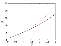
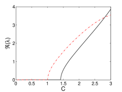
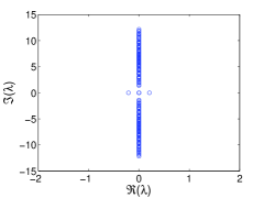
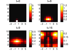
Figure 1: (Color online) Dynamical features of the fundamental surface soliton. The top left and right panels show, respectively, the soliton’s norm, $P$, and the real part of the critical stability eigenvalue, versus the lattice coupling, $C$. For comparison, the dash-dotted lines show respective quantities for a fundamental soliton in the uniform lattice. The instability is due to an eigenvalue pair bifurcating from the edge of the phonon band, that eventually crosses the origin of the spectral plane and becomes real. In the bottom panels, we display the linear-stability spectrum of a single-site soliton, and snapshots of its evolution (contour plots of $|u_{m,n}|^{2}$), for $C=1.43$, slightly above the instability threshold.

III Numerical results

To examine the existence and stability of the above configurations numerically, we start with the fundamental onsite soliton at the surface, (a). Basic results for this state are displayed in Fig. 1. At $C=0$, there is a double zero eigenvalue due to the phase invariance. For small $C>0$, this is the only eigenvalue of the linearization near the origin of the spectral plane $(\Re(\lambda),\Im(\lambda))$. As $C$ increases, one encounters a critical value, at which an additional (but still marginally stable) eigenvalue bifurcates from the edge of the continuous spectrum, as mentioned above. With the further increase of $C$, this bifurcating eigenvalue arrives at the origin of the spectral plane, and subsequently gives rise to an unstable eigenvalue pair, with $\Re(\lambda)\neq 0$, see Fig. 1. This happens for $C>1.41$; we note in passing that the results reported herein have been obtained for lattices of size $10\times 10$, but it has been verified that a similar phenomenology persists for larger lattices of up to $25\times 25$. For comparison, we also display, by a dashed-dotted line, the critical unstable eigenvalue for a fundamental soliton on the uniform lattice (as a matter of fact, for a soliton sitting far from the edge), which demonstrates that the interaction with the edge leads to conspicuous expansion of the stability interval of the fundamental soliton. This may also be justified intuitively, as the instability of the fundamental soliton emerges closer to the continuum limit which is well-known to be unstable to (very slow) collapse type phenomena. A surface variant of the relevant structure enjoys the company of fewer neighboring sites and hence is “more slowly” (in parameter space) approaching its continuum limit, in comparison with its infinite lattice sibling.

Development of the instability of the fundamental surface soliton (in the case when it is unstable) was examined in direct simulations of Eq. (1). As seen in Fig. 1, in this case the excitation propagates away from the edge, expanding into an apparently disordered state. This is justifiable as for this parametric regime there is no stable localized state neither in the vicinity of the surface or in the (more unstable) bulk of the uniform lattice.

  

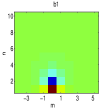
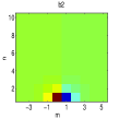
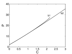
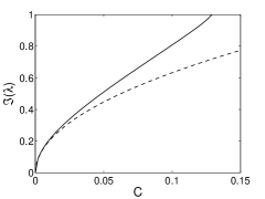
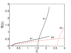
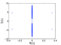
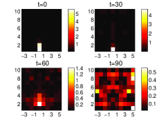
Figure 2: (Color online) Top panels: Vertical (b1) and horizontal (b2) dipoles, which, at $C=0$, are seeded through Eq. (3). The top left and middle panels show examples of these dipoles at $C=1$, and the right panel shows their norms. Middle and bottom panels: The same as Fig. 1, but for the configurations b1 and b2. The vertical dipole, b1, disappears via a saddle-node bifurcation at $C\approx 2.17$. The left middle panel displays the eigenvalue bifurcating from zero at $C=0$, the dashed line being the analytical approximation described in the text, i.e., $\Im(\lambda)=2\sqrt{C}$. The right middle panel shows the onset of the b1 (solid lines) and b2 (dashed lines) instabilities for the dipole modes, as found from numerical computations. An example of the spectrum and nonlinear evolution of an unstable vertical dipole are presented in the bottom panels, for $C=1$.

Next, in Fig. 2 we present results for the vertical and horizontal dipoles, (b1) and (b2) (see top left and middle panels of Fig. 2, seeded as per Eq. (3). At $C=0$, the dipole has two pairs of zero eigenvalues, one of which becomes finite (remaining stable) for $C>0$, as shown above in the analytical form. Our numerical findings reveal that, in compliance with the analytical results, the dipoles of both types give rise to virtually identical finite eigenvalues (hence only one eigenvalue line is seen in the left middle panel of Fig. 2). As seen in the right middle panel in Fig. 2, both dipoles lose their stability simultaneously, at $C\approx 0.15$. Continuing the computations past this point, we conclude that the vertical and horizontal dipoles become different when $C$ attains values $\sim 1$. Eventually, the (already unstable) vertical configuration, b1, disappears in a saddle-node bifurcation at $C\approx 2.17$, while its horizontal counterpart, b2, persists through this point. Furthermore, there is a critical value of $C$ at which an eigenvalue bifurcates from the edge of the continuous spectrum. Eventually, this bifurcating eigenvalue crosses the origin of the spectral plane, giving rise to an unstable eigenvalue pair, with $\Re(\lambda)\neq 0$. The value of $C$ at which this secondary instability sets in is essentially smaller for b1, i.e., $C\approx 1.55$, than $C\approx 2.61$ for b2. We thus conclude that the horizontal dipole, b2, is, generally, more robust than its vertical counterpart, b1. This conclusion seems natural, as the proximity to the edge stabilizes the fundamental soliton (as shown above), and in the horizontal configuration the two sites that constitute the dipole are located closer to the border.

Nonlinear evolution of unstable dipoles was examined too, in direct simulations. As seen in the example (for configuration b1) shown in the bottom panels of Fig. 2, the instability again results in a disordered state.

Proceeding to the completely novel configuration (c) of the horseshoe, we note that, because it was seeded at three sites when $C=0$, there are three pairs of zero eigenvalues in the AC limit. Above, it was shown analytically that one pair of these eigenvalues becomes finite at order $\mathcal{O}(C)$, and another at $\mathcal{O}(C^{2})$. Numerical results demonstrate that the first pair remains stable until it collides with the edge of the continuous spectrum, which happens at $C\approx 0.25$. As mentioned above, the second eigenvalue pair, bifurcating from zero at order $\mathcal{O}\left(C^{2}\right)$, is critical for the stability of configuration (c). The numerical results show that this pair bifurcates into a stable (i.e., imaginary) one, and, as shown in Fig. 3, the horseshoe remains stable up to $C\approx 0.25$.

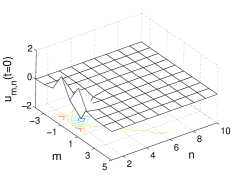
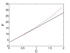
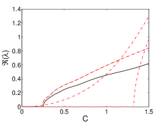
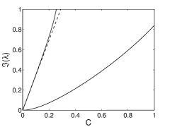
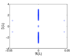
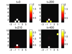
Figure 3: (Color online) The same as Fig. 2 for the “horseshoe” configuration, Eq. (4). The top panels show an example of the structure and its norm as a function of $C$ (black solid curve). The solid curves in the middle panels display the real and imaginary parts of the key stability eigenvalues (the dashed line in the right middle panel is the analytical approximation for the imaginary part presented in the text). For comparison, the red dash-dotted lines show the same characteristics for a family of horseshoe solitons created in the uniform lattice. It is seen that the latter family is completely unstable, while the same waveform trapped at the edge of the lattice has a well-defined stability region. This is a remarkable consequence of the presence of the surface. The bottom panels present the linear instability spectrum of the horseshoe state with $C=0.26$, and its evolution in time.

To understand the effect of the surface on the stability of the horseshoes, it is relevant to compare them to their counterparts in the infinite lattice, i.e., similar structures that may be created, starting from the AC limit taken as per Eq. (4), far from the domain edge. By itself, the latter is a novel family of localized solutions to the DNLS equation in 2D. However, the important feature is that, the structure in the bulk of the uniform lattice (unlike the quadrupole that may be stable), is unstable for the entire family of horseshoes [in fact, the $\mathcal{O}(C^{2})$ eigenvalue pair, bifurcating from zero at $C=0$, immediately becomes real in this case, see the corresponding, quadratically growing dashed-dotted line in the left middle panel in Fig. 3]. Thus, the horseshoe attached to the surface is another example of the localized mode stabilized by the lattice’s edge (however, unlike the above example of the stabilized fundamental soliton, the dependence of the horseshoe’s stability on the border is crucial, as it may never be stable in the infinite lattice).

The bottom panels of Fig. 3 exemplify the evolution of the horseshoe when it is unstable. Unlike the situations with configurations (a) and (b), the unstable horseshoe does not decay into a disordered state, but rather splits into a pair of two fundamental solitons (with $S=0$), one trapped at the surface and one found deeper inside the lattice.

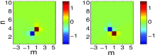
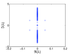
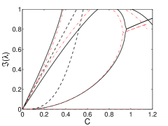
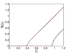
Figure 4: (Color online) The supersymmetric vortex cell seeded as per Eq. (13). The top left and right panels show, respectively, the real and imaginary parts of the solution and its (in)stability spectrum for $C=0.4$. The bottom panel displays imaginary and real parts of the stability eigenvalues versus $C$. The solid and dashed lines show numerical and analytical results for small $C$. For comparison, red dashed-dotted lines depict the same numerically found characteristics for a supersymmetric vortex on the infinite lattice.

IV Surface effect on the existence of vortices

Besides the stabilization effect reported above, the lattice edge may exert a different effect, impeding the existence of some solutions. As an example, we consider the, so-called supersymmetric peli05 , lattice vortex attached to the edge, i.e., one with the vorticity ($S=1$) equal to the size of the square which seeds the vortex at $C=0$, through the following set of four excited sites, cf. Eq. (4):

$$\left\{v^{(0)}_{0,1},v^{(0)}_{1,1},v^{(0)}_{1,2},v^{(0)}_{0,2}\right\}=\left\{e^{i\theta_{0,1}},e^{i\theta_{1,1}},e^{i\theta_{1,2}},e^{i\theta_{0,2}}\right\},$$ (12)

with $\theta_{0,1}=0$, $\theta_{1,1}=\pi/2$, $\theta_{1,2}=\pi$, and $\theta_{0,2}=3\pi/2$ (unlike the above configurations, this one is not a purely real one). While supersymmetric vortices exist in uniform lattices (including anisotropic ones) and have their own stability regions there peli05 ; we3 , numerical analysis shows that the localized mode initiated as per Eq. (12) in the model with the edge cannot be continued to $C>0$. In fact, we have found that, to create such a state at finite $C$, we need to seed it, at least, two sites away from the edge, i.e., as

$$\left\{v^{(0)}_{0,3},v^{(0)}_{1,3},v^{(0)}_{1,4},v^{(0)}_{0,4}\right\}=\left\{e^{i\theta_{0,3}},e^{i\theta_{1,3}},e^{i\theta_{1,4}},e^{i\theta_{0,4}}\right\}.$$ (13)

[the set on the right-hand side is a translated version of that of Eq. (12)]. Numerically found stability eigenvalues for this structure are presented in Fig. 4, along with the analytical approximation, obtained by means of the same method as above. In all, there are 4 pairs of analytically predicted eigenvalues near the spectral plane origin (given the four initial seed sites of the configuration). More specifically, these are:  $\lambda=0$ (associated with the phase invariance), $\lambda=\pm 2Ci$ (a double eigenvalue pair), and $\lambda=\pm\sqrt{32}C^{3}i$ (a higher order eigenvalue pair). As it can be seen in the figure, already at this distance of two sites from the boundary, the behavior is sufficiently close to that of an infinite lattice.

V Conclusion

We have demonstrated that properties of fundamental localized modes in the 2D lattice with an edge may be drastically different from well-known features in the uniform lattice. In particular, the edge helps to increase the stability region for the ordinary solitons, and induces a difference between dipoles oriented perpendicular and parallel to the lattice’s border. Additionally, regular supersymmetric vortices cannot be created too close to the border. Most essentially, the edge stabilizes a new species of solitons which is entirely unstable in the uniform lattice, the so-called “horseshoe solitons”. In that sense, the presence of the surface may produce a very desirable “stability broadening” impact on a number of different solutions; this may become especially interesting in applications related to waveguide arrays, among other optical or soft-matter systems.

Natural issues for further consideration are horseshoes of a larger size, and counterparts of such localized modes in 3D lattices near the edge. In the 3D lattice, one can also consider solitons in the form of vortex rings or cubes we4 set parallel to the border.

PGK gratefully acknowledges support from NSF-DMS-0204585, NSF-CAREER. RCG and PGK also acknowledge support from NSF-DMS-0505663.

References

- (1) R. K. Dodd, J. C. Eilbeck, J. D. Gibbon, and H. C. Morris. Solitons and nonlinear wave equations (Academic Press, London, 1982).
- (2) G. Maugin. Nonlinear Waves in Elastic Crystals (Oxford University Press: Oxford, 2000).
- (3) L. Stenflo, Physica Scripta T63, 59 (1996).
- (4) K. G. Makris, S. Suntsov, D. N. Christodoulides, G. I. Stegeman, and A. Hache, Opt. Lett. 30, 2466 (2005); M. I. Molina, R. A. Vicencio, and Y. S. Kivshar, Opt. Lett. 31, 1693 (2006).
- (5) S. Suntsov, K. G. Makris, D. N. Christodoulides, G. I. Stegeman, A. Haché, R. Morandotti, H. Yang, G. Salamo, and M. Sorel, Phys. Rev. Lett. 96, 063901 (2006).
- (6) I. L. Garanovich, A. A. Sukhorukov, Y. S. Kivshar, and M. Molina, Opt. Express 14, 4780 (2006).
- (7) M. I. Molina, Phys. Rev. B 71, 035404 (2005); ibid. 73, 014204 (2006).
- (8) Y. V. Kartashov, L. Torner and V. A. Vysloukh, Phys. Rev. Lett. 96, 073901 (2006).
- (9) C. R. Rosberg, D. N. Neshev, W. Krolikowski, A. Mitchell, R. A. Vicencio, M. I. Molina, and Y. S. Kivshar, e-print physics/0603202.
- (10) G. A. Siviloglou, K. G. Makris, R. Iwanow, R. Schiek, D. N. Christodoulides, G. I. Stegeman, Y. Min, and W. Sohler, Opt. Exp. 14, 5508 (2006).
- (11) Y. V. Kartashov, A. A. Egorov, V. A. Vysloukh, and L. Torner, Opt. Express 14, 4049 (2006).
- (12) B. A. Malomed and P. G. Kevrekidis, Phys. Rev. E 64, 026601 (2001).
- (13) D. N. Neshev, T. J. Alexander, E. A. Ostrovskaya, and Y. S. Kivshar, H. Martin, I. Makasyuk, and Z. Chen, Phys. Rev. Lett. 92, 123903 (2004); J. W. Fleischer, G. Bartal, O. Cohen, O. Manela, M. Segev, J. Hudock, and D. N. Christodoulides, Phys. Rev. Lett. 92, 123904 (2004).
- (14) M. I. Molina, e-print nlin.PS/0604060.
- (15) Y. V. Kartashov, private communication.
- (16) D. E. Pelinovsky, P. G. Kevrekidis and D. J. Frantzeskakis, Physica D 212, 20 (2005).
- (17) P. G. Kevrekidis, B. A. Malomed, and A. R. Bishop, J. Phys. A: Math. Gen. 34, 9615 (2001).
- (18) J. Yang, I. Makasyuk, A. Bezryadina, and Z. G. Chen, Stud. Appl. Math. 113, 389 (2004); Z. G. Chen, H. Martin, E. D. Eugenieva, J. J. Xu, and J. K. Yang, Opt. Express 13, 1816 (2005).
- (19) P. G. Kevrekidis, B. A. Malomed, Z. Chen, and D. J. Frantzeskakis, Phys. Rev. E 70, 056612 (2004); H. Sakaguchi and B. A. Malomed, Europhys. Lett. 72, 698 (2005).
- (20) P. G. Kevrekidis, D. J. Frantzeskakis, R. Carretero-González, B. A. Malomed, and A. R. Bishop, Phys. Rev. E 72, 046613 (2005).
- (21) P. G. Kevrekidis, B. A. Malomed, D. J. Frantzeskakis and R. Carretero-González, Phys. Rev. Lett. 93, 080403 (2004); R. Carretero-González, P. G. Kevrekidis, B. A. Malomed and D. J. Frantzeskakis, ibid. 94, 203901 (2005).