Chaotic Dynamics in Optimal Monetary Policy
Abstract
There is by now a large consensus in modern monetary policy. This consensus has been built upon a dynamic general equilibrium model of optimal monetary policy as developed by, e.g., Goodfriend and King (1997), Clarida et al. (1999), Svensson (1999) and Woodford (2003). In this paper we extend the standard optimal monetary policy model by introducing nonlinearity into the Phillips curve. Under the specific form of nonlinearity proposed in our paper (which allows for convexity and concavity and secures closed form solutions), we show that the introduction of a nonlinear Phillips curve into the structure of the standard model in a discrete time and deterministic framework produces radical changes to the major conclusions regarding stability and the efficiency of monetary policy. We emphasize the following main results: (i) instead of a unique fixed point we end up with multiple equilibria; (ii) instead of saddle–path stability, for different sets of parameter values we may have saddle stability, totally unstable equilibria and chaotic attractors; (iii) for certain degrees of convexity and/or concavity of the Phillips curve, where endogenous fluctuations arise, one is able to encounter various results that seem intuitively correct. Firstly, when the Central Bank pays attention essentially to inflation targeting, the inflation rate has a lower mean and is less volatile; secondly, when the degree of price stickiness is high, the inflation rate displays a larger mean and higher volatility (but this is sensitive to the values given to the parameters of the model); and thirdly, the higher the target value of the output gap chosen by the Central Bank, the higher is the inflation rate and its volatility.
keywords:
Optimal monetary policy, Interest Rate Rules, Nonlinear Phillips Curve, Endogenous Fluctuations and StabilizationIntroduction
Since the early 1990s we have witnessed an increasing consensus in the conduct of modern monetary policy. Goodfriend and King (1997) have labelled this new consensus as ”The New Neoclassical Synthesis and the Role of Monetary Policy”, while Clarida et al. (1999) called it the ”The Science of Monetary Policy: A New Keynesian Perspective”. This new framework is a natural extension of the seminal idea developed by Taylor (1993), in which the central bank should conduct monetary policy through an aggressive and publicly known rule with commitment. In fact, this emerging consensus turned upside down the basic prescriptions of monetary and fiscal policies of the old Neoclassical Synthesis of the 60’s and 70’s, and has led to a standard DGEM so successful that, as Laurence Ball has recently commented, ”the model is so hot that the Keynesians and Classicals fight over who gets credit for it” (2005, 265).
In this paper we extend the standard model by introducing nonlinearity into the Phillips curve. As the linear Phillips curve seems to be at odds with empirical evidence and basic economic intuition, a similar procedure has already been undertaken in a series of papers over the last few years, e.g., Schaling (1999), Semmler and Zhang (2004), Zhang and Semmler (2003), Nobay and Peel (2000), Tambakis (1999), and Dolado et al. (2004). However, these papers were mainly concerned with analyzing the problem of inflation bias, deriving an interest rate rule which is nonlinear. The issue of stability and the possible existence of endogenous cycles in such a framework were totally overlooked in these papers. One possible justification for this fact is the type of nonlinearity that is introduced into the standard model, because, as it is well known in the literature, quadratic preferences by the central bank with a convex Phillips Curve, as the one used by most of those papers, do not secure closed form solutions.
In contrast, under the specific form of nonlinearity proposed in our paper, which allows for convexity and concavity and secures closed form solutions, we show that the introduction of a nonlinear Phillips curve into the structure of the standard model in a discrete time and deterministic framework produces radical changes to the major conclusions regarding stability and the efficiency of monetary policy under the new framework.
1 The Model
Assume that the Central Bank has quadratic loss preferences over the rate of inflation and the output gap . It’s objective is to minimize the squared errors of these two state variables with respect to their target values fixed and publicly announced by the bank
| (1) |
where is the Central Bank objective function and is the relative weight of the output gap in the bank’s loss function, is the expectation operator, and is the gross rate of intertemporal discount. It should be also stressed that the parameters that reflect the options of the Central Bank concerning optimal monetary policy are essentially three in this model: and Firstly, if , then the Central Bank is only concerned about the control of inflation, with no concern at all about real variables like the output gap, employment, or consumption. Secondly, if the Central Bank wants to achieve an expected value of output exactly equal to the long term trend value of such variable. Thirdly, if then the Central Bank aims to achieve an expected value for the rate of inflation that is zero over time.
The objective function is optimized subject to two constraints. The first is a forward looking Investment-Savings function (IS function) derived from an optimal intertemporal problem in which families evaluate the trade-off between consumption vs savings and leisure vs labour and is given by
| (2) |
where stands for the nominal interest rate; is the private sector expected rate of inflation at ; is the expected output gap at and stands for aggregate demand shocks (e.g. changes in government expenditures) and defined as an autoregressive Markov process: . Notice that the term gives the level of the real expected interest rate, and is the interest elasticity with respect to the output gap. Moreover, notice also that in this optimal control problem the rate of interest () is the control or co-state variable of the problem.
The second constraint is an aggregate supply function describing the behavior of firms. It is presented as a new Keynesian Phillips curve, and in fact it is the old Phillips Curve but now derived from microeconomic principles. Following Calvo (1983), at time only a proportion of firms can adjust prices due to market imperfections, which leads to the following supply function
| (3) |
where is also defined by a Markov process,
Notice that the standard model assumes to be linear, where represents the level of price stickiness in the economy (which is decreasing in such that the higher is , the lower is the level of price rigidity.
The optimal intertemporal problem consists in optimizing (1) subject to constraints (2) and (3). The problem can be solved using the usual tools of dynamic optimization. To maximize the objective function of the Central Bank the current value Hamiltonian takes the form
where and are shadow-prices associated with and , respectively. Notice that, the expectations operators for next period inflation and output gap and the stochastic factors have been removed in the Hamiltonian, because from now onwards we assume two crucial assumptions: (i) we will work under a deterministic framework, and (ii) agents are fully rational. The adoption of these two assumptions leads to a fully deterministic perfect foresight equilibrium and in practical terms it means that and .
First order necessary conditions are
| (5) | |||||
| (6) | |||||
| (7) | |||||
| (8) |
Simple manipulation of these conditions allow us to arrive at the first equation of the reduced form of our system
| (9) |
while the second equation is given by the Phillips curve.
1.1 The nonlinear case
We consider two alternative cases for the introduction of nonlinearity into the Phillips curve. The two cases can be separately analyzed and they depend essentially on whether the currently perceived output gap by the Central Bank is higher than its target value ( or lower than the perceived value (. Defining a positive parameter , the two specific nonlinear functions are
Notice that the two above functions contain the properties required for our Phillips curve. First, for , the functions are identical and we are back to the linear case (). Second, the function can be either concave or convex for both cases depending on the value of and on whether the initial condition is to the left/right of the target value of the output gap. Third, regarding the nonlinear functions presented in the literature previously referred to, these functions have the advantage of allowing for closed form solutions which can be treated in an analytical way, and moreover, they also lead to both positive and negative values of the output gap.
Under the specific nonlinear functions chosen for , the following two systems should be evaluated in order to derive any results from the model.
i) :
| (10) | |||||
ii) :
| (11) | |||||
Systems (10) and (11) change significantly the results of the monetary policy problem as far as the standard model is concerned. It can be shown that for several sets of parameter values the nonlinear model leads to multiple equilibria, and large instability arising from deterministic endogenous cycles. As we can see in both systems, the power of the second equation shows that there are always two equilibria in each case. However, due to space limitations, we are forced to illustrate here only one equilibrium point of the second case above referred to (where ) as this case is the one that is usually most found in contemporary economics.
2 Local and global dynamics
In this section we present the dynamic behavior of the system defined in (11). There are two real equilibrium points but only one is compatible with reasonable parameter value restrictions. This equilibrium point is analytically determined and discussed in what follows. Saddle-node bifurcations are possible and a Neimark-Sacker (or torus breakdown) bifurcation route to chaos is encountered when the parameter is varied. Since we have power functions we have to consider positive square powers in order to ensure the existence of real iterations. This is the reason why in the numerical examples presented below we almost always assume (which gives
2.1 The case:
Proposition 1
The dynamic system (11) has always an unstable equilibrium given by the following point
Proof. The stability of this fixed point is analyzed using the sufficient conditions, where is the Jacobian matrix computed at the fixed point. We have then
where
This means that there is no stable equilibrium, independently of the value of .
Analogous to the first model if we solve the conditions
we may obtain the first period-doubling bifurcation location, the Neimark-Sacker and the Saddle-Node bifurcation points. For
there is a period-doubling bifurcation (again, the result is not relevant, because it implies a strong degree of nonlinearity). For
we have a saddle-node bifurcation and for there is a Neimark-Sacker bifurcation.
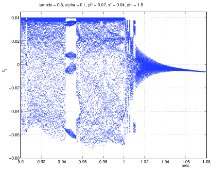
We assume the following parameter calibration: , and let for now the parameter to vary in order to study how this parameter affects the global dynamics of the model. As it is shown in Figure 1, when is varied the dynamics is characterized by high order Neimark-Sacker bifurcations, breakdown of closed invariant curves, stretching and folding, and all this route leads the system to settle down in chaotic dynamics.
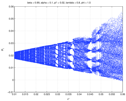
Let us assume that in order to study the impact of variations on two other fundamental parameters of the model: , . When we vary these two parameters in the interval the system is also always chaotic, with eigenvalues with modulus greater than 1; which means that the first bifurcations occur for parameter values outside the given intervals. Figure 2 shows the complex motion of the model, where some stability windows, quasi-regular and chaotic motion can be observed.
We may also analyze the impact upon the dynamics if the central bank decides to accept higher target values for the output gap Figure 3 shows the bifurcation diagram of the variable when is increased, illustrating several stability windows, where high order Neimark-Sacker bifurcations take places. In these windows several closed invariant curves start to stretch and fold, and after all breakdown and join in a chaotic attractor. We can also observe the increasing of volatility in the inflation rate if the central bank fixes a target value for the output gap relatively high.
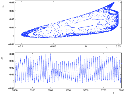
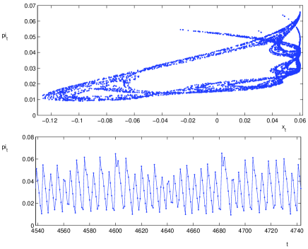
Finally, Figures 4 and 5 show the attractor and the correspondent time series of the rate of inflation for the calibration above presented, with a small difference. While the former assumes all the values of the calibration, including the values for the target variables , the latter takes a slightly change in the values of these parameters . The initial conditions are so that the condition is satisfied. Two points should be highlighted. First, the time series show figures for the rate of inflation that are not far from those we find in contemporary advanced economies. Secondly, the mean of the rate of inflation in each simulation is very close to the target value of the Central Bank; however, there is significant volatility showing that the bank may have some control on inflation but it is very hard to control the rate in a very efficient way (that is, to reduce or eliminate the volatility in inflation).
3 Conclusions
A nonlinear Phillips curve produces radical changes to the major conclusions regarding stability and the efficiency of monetary policy. The main results are the following: (i) instead of a unique fixed point we end up with multiple equilibria; (ii) instead of saddle–path stability, for different sets of parameter values we may have saddle stability, totally unstable equilibria and chaotic attractors; (iii) for certain degrees of convexity and/or concavity of the Phillips curve, where endogenous fluctuations arise, one is able to encounter some results that seem intuitively correct. Firstly, when the Central Bank pays attention essentially to inflation targeting, the inflation rate has a lower mean and is less volatile (as one can see in the upper panel of Figure 2). Secondly, changes in the degree of price stickiness may (or may not) affect the levels of the mean and the variance of the inflation rate, depending on the specific values of the various parameters (see the lower panel of Figure 2). Thirdly, the higher the target value of the output gap chosen by the Central Bank, the higher is the inflation rate and its volatility (see Figure 3).
Moreover, the existence of endogenous cycles due to chaotic motion may raise serious questions about whether the old dictum of monetary policy (that the Central Bank should conduct policy with some level of discretion instead of pure commitment) is not still in the business of monetary policy.
Acknowledgements: Financial support from the Fundação Ciência e Tecnologia, Lisbon, is grateful acknowledged, under the contract No POCTI/ ECO/ 48628/ 2005, partially funded by the European Regional Development Fund (ERDF).
References
- [1] Ball, L. (2003). ”Comments on the Monetary Policy Debate since October 1979”, Federal reserve Bank of St. Louis Review, 87(2), Part 2, 263-268.
- [2] Calvo, G. (1983). “Staggered Prices in a Utility Maximizing Framework.” Journal of Monetary Economics, vol. 12, 383-398.
- [3] Clarida, R.; J. Gali and M. Gertler (1999). ”The Science of Monetary Policy: a New Keynesian Perspective.” Journal of Economic Literature, vol. 37, 1661-1707.
- [4] Dolado, J.; R. Pedrero and F. J. Ruge-Murcia (2004). ”Nonlinear Monetary Policy Rules: Some New Evidence for the U.S.” Studies in Nonlinear Dynamics Econometrics, vol. 8, issue 3, article 2, 1-32.
- [5] Goodfriend, M. and R. G. King (1997). ”The New Neoclassical Synthesis and the Role of Monetary Policy.” in Ben Bernanke and Julio Rotemberg (eds.), NBER Macroeconomics Annual 1997, Cambridge, Mass.: MIT Press, 231-282.
- [6] Nobay, A. and Pell, D. ”Optimal Monetary Policy with a Nonlinear Phillips Curve”, Economics Letters, 67, 159-164.
- [7] Schaling, E. (1998). ”The Nonlinear Phillips Curve and Inflation Forecast Targeting.” Bank of England working paper no 98.
- [8] Semmler, W. and W. Zhang (2004). ”Monetary Policy with Nonlinear Phillips Curve and Endogenous NAIRU.” Center for Empirical Macroeconomics, Bielefeld.
- [9] Svensson, L. E. O. (1999b). ”Inflation Targeting as a Monetary Policy Rule.” Journal of Monetary Economics, vol. 43, 607-654.
- [10] Tambakis, D. N. (1999). ”Monetary Policy with a Nonlinear Phillips Curve and Asymmetric Loss.” Studies in Nonlinear Dynamics and Econometrics, vol. 3, 223-237.
- [11] Taylor, J. B. (1993). “Discretion versus Rules in Practice.” Carnegie-Rochester Series on Public Policy, vol. 39, 195-214.
- [12] Woodford, M. (2003). Interest and Prices: Foundations of a Theory of Monetary Policy. Princeton, New Jersey: Princeton University Press.
- [13] Zhang, W. and W. Semmler (2003). ”Monetary Policy under Model Uncertainty: Empirical Evidence, Adaptive Learning and Robust Control.” Center for Empirical Macroeconomics, Bielefeld.