Two-dimensional nonlocal multisolitons

Abstract

We study the bound states of two-dimensional bright solitons in nonlocal nonlinear media. The general properties and stability of these multisolitary structures are investigated analytically and numerically. We have found that a steady bound state of coherent nonrotating and rotating solitary structures (azimuthons) can exist above some threshold power. A dipolar nonrotating multisoliton occurs to be stable within the finite range of the beam power. Azimuthons turn out to be stable if the beam power exceeds some threshold value. The bound states of three or four nonrotating solitons appear to be unstable.

The recent experimental observations of spatial solitons in nonlocal media such as nematic liquid crystals [1, 2], lead glasses [3], renewed an interest to coherent structures in spatially nonlocal nonlinear media. In the spatially nonlocal media the nonlinear response depends on the wave packet intensity at some extensive spatial domain. Nonlocality is a key feature of many nonlinear media. It naturally appears in different physical systems such as plasmas [4, 5, 6], Bose- Einstein condensates [7], optical media [8], liquid crystals [1], and soft matter [9]. Different types of single (solitons , vortices) and composite (soliton clusters) solitary structures have been predicted and experimentally observed in various nonlinear media [10]. Rotating scalar multipoles (azimuthons) were first introduced in Ref. [11] for models with local nonlinearity.

A composite soliton structure, or a multi-soliton complex is a self-localized state which is a nonlinear superposition of several fundamental solitons. Stationary multi-soliton structures in nonlocal media were considered first in Refs. [12, 13]. However, a question of the stability of the multisolitons is still an open problem. In particular, the form of the nonlinear nonlocal response is crucial for the multisoliton stability. Stable two-dimensional (2D) rotating [14] and nonrotating [15] dipole solitons in a medium with Gaussian response function have been numerically observed. Authors of Refs. [16] investigated a more realistic model with the Helmholtz type response function (often referred to as the model with thermal nonlinearity) and showed that multipole vector solitons can be made stable. This model describes, in particular, the nonlinear nonlocal response of some thermo-optical materials, liquid crystals, and partially ionized plasmas [1, 3, 5]. Very recently experimental observation of scalar multipole solitons in the optical media with thermal nonlocal nonlinearity has been reported [17]. It is particularly remarkable that all multisolitons investigated in Ref. [17] are found to be unstable, but with a large parameters range where the instability is weak, so that their experimental observation is possible. In this Letter, using direct 2D simulations for a scalar model with thermal nonlocal nonlinearity, we find a class of radially asymmetric nonrotating two-dimensional soliton solutions and show that, at some input power, the dipole-mode scalar solutions are stable, while the tripoles and quadrupoles are always unstable, but can survive over quite considerable distances. The stability window for dipolar multisolitons is found. We find also rotating dipole and quadrupole solutions (azimuthons) which turn out to be stable if the beam power exceeds some threshold value.

The basic system of equations, written in appropriate dimensionless variables, is

$$i\frac{\partial\Psi}{\partial z}+\Delta_{\perp}\Psi+\theta\Psi=0,$$ (1)

$$\alpha^{2}\theta-\Delta_{\perp}\theta=|\Psi|^{2},$$ (2)

where $\Delta_{\perp}=\partial^{2}/\partial x^{2}+\partial^{2}/\partial y^{2}$ is the transverse Laplacian. Equations (1) and (2) describe the propagation in $z$-direction of the electric field envelope $\Psi(x,y,z)$ coupled to the temperature perturbation $\theta(x,y,z)$ in a plasma [5]. The identical model describes the wave field $\Psi$ and spatial distribution of the molecular director $\theta$ in nematic liquid crystals [1].

The parameter $\alpha$ stands for the degree of nonlocality of the nonlinear response. In the limit $\alpha^{2}\gg 1$, Eqs. (1) and (2) reduce to the usual nonlinear Schrödinger equation; the opposite case $\alpha^{2}\ll 1$ corresponds to a strongly nonlocal regime. For plasmas parameter $\alpha$ characterizes the relative energy that electron with mass $m$ delivers to a heavy particle with mass $M$ during single collision ($\alpha^{2}\approx 2m/M$). Therefore, the thermal self-focusing in a plasma occurs in a strongly nonlocal regime. The model used in Ref. [3] to describe the propagation of the wave beam in optical media with thermal nonlinearity corresponds to the specific nonlocal limit $\alpha\to 0$. In nematic liquid crystals, the degree of nonlocality can be modulated by changing the pretilt angle $\theta_{0}$ of molecules through bias voltage $V$ [18]. As $V$ increases, the degree of nonlocality decreases, so that the degree of nonlocality can be tuned from local regime to a strongly nonlocal one.

Equations (1) and (2) can be rewritten as a single integro-differential equation

$$i\frac{\partial\Psi}{\partial z}+\Delta_{\perp}\Psi+\Psi\int R(|\mathbf{r}-\mathbf{r}^{\prime}|)|\Psi(\mathbf{r}^{\prime})|^{2}\,d\mathbf{r}^{\prime}=0,$$ (3)

with the kernel $R(\xi)=K_{0}(\alpha\xi)/(2\pi)$, where $K_{0}(z)$ is the modified Bessel function of the second kind of order zero. It is seen, that the nonlinearity in Eq. (3) has essentially nonlocal character.

We look for stationary solutions of Eqs. (1) and (2) in the form $\Psi(x,y,z)=\psi(x,y)\exp(i\lambda z)$, so that $\psi(x,y)$ obeys the equations

$$-\lambda\psi+\Delta_{\perp}\psi+\theta\psi=0,$$ (4)

$$\alpha^{2}\theta-\Delta_{\perp}\theta=|\psi|^{2},$$ (5)

and we do not assume the radial symmetry of $\psi(x,y)$. For the numerical modeling we use the rescaled variables $\psi\rightarrow\psi/\alpha$, $\theta\rightarrow\theta/\alpha^{2}$, $z\rightarrow z\alpha^{2}$, $(x,y)\rightarrow(x,y)\alpha$, $\lambda\rightarrow\lambda/\alpha^{2}$, so that $\alpha=1$ in Eqs. (4) and (5). Note, a strongly nonlocal regime ($\alpha\ll 1$) corresponds to large values of the scaled propagation constant $\lambda$. Imposing periodic boundary conditions on Cartesian grid and choosing an appropriate initial guess we have found a class of radially asymmetric multipole localized solutions by using the relaxation technique similar to one described in Ref. [19]. The real (or containing only a constant complex factor) function $\psi(x,y)$ corresponds to nonrotating solitary structures. Examples of such nonrotating multipole solitons, namely, a dipole, a tripole, and a quadrupole are presented in Fig. 1. The nonrotating multipoles consist of several fundamental solitons (monopoles) with opposite phases. The complex function $\psi(x,y)$ with a spatially modulated phase corresponds to rotating structures (azimuthons) with nonzero angular momentum. In Fig. 2 we demonstrate two examples of the azimuthons for the nonlocal model described by Eqs. (1) and (2).

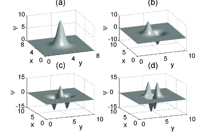
Figure 1: Numerically found stationary localized nonrotating solutions of Eqs. (4) and (5): (a) monopole with $\lambda=10$; (b) dipole with $\lambda=10$; (c) tripole with $\lambda=15$; (d) quadrupole with $\lambda=20$.

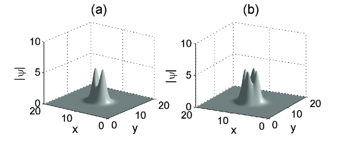
Figure 2: Two examples of the azimuthons with $\lambda=4.5$. Intensity $|\psi|$ is shown in the $(x,y)$ plane. a) solution with two intensity peaks; b) solution with four intensity peaks.

To gain the better insight into the properties of the stationary nonrotating multisolitons we have performed the analytical variational analysis. A stationary nonrotating multisoliton can be described by the trial function of the form:

$$\Psi(x,y,z)=hf(x,y)e^{i\lambda z},$$ (6)

where the shape of the dipolar multisoliton can be approximated by the antisymmetric superposition of two gaussian functions:

$$f(\xi,\eta)=e^{-\frac{1}{2a^{2}}\left\{y^{2}+(x-d/2)^{2}\right\}}-e^{-\frac{1}{2a^{2}}\left\{y^{2}+(x+d/2)^{2}\right\}},$$

where $a$ and $d$ characterize the radius of each monopoles and the distance between them, respectively. For the bound state of $S$ identical single solitons with the centers at $(x_{s},y_{s})$, where $s=1\dots S$, we have used the trial function of the form:

$$f(\xi,\eta)=\sum_{s=1}^{S}g_{s}e^{-\frac{1}{2}(\xi-\xi_{s})^{2}-\frac{1}{2}(\eta-\eta_{s})^{2}},$$

where $(\xi,\eta)=(x,y)/a$, $g_{s}=\pm 1$ gives the phase of the $s$-th soliton.

As known, the steady-state corresponds to the stationary point of the Hamiltonian

$$H=\int\left\{|\nabla_{\perp}\Psi|^{2}-\frac{1}{2}\theta|\Psi|^{2}\right\}d^{2}\textbf{r}$$ (7)

at the fixed number of quanta $N$

$$N=\int|\Psi|^{2}d^{2}\textbf{r}.$$ (8)

In the variational approach, Hamiltonian $H(a,b)$ is the function of two variational parameters $a$ and $b=d/a$, where $a$ characterizes the width of each monopole and $d$ is the distance between two neighboring out-of-phase solitons. The third parameter of the trial function (6), the amplitude $h$, has been eliminated in terms of $a$, $b$, and $N$ using the normalization condition (8).

Results of the variational analysis are found to be in very good agreement with our numerical simulations for stationary nonrotating multisolitons. Figure 3 (a) shows the beam power $N$ versus the propagation constant $\lambda$ for monopoles, dipoles, tripoles, and quadrupoles. The threshold power for existence of the stationary bound state of $S$ solitons is very close to the threshold for formation of $S$ single unbound fundamental solitons. Moreover, the ”binding energy” $N_{S}-SN_{1}$ (where $N_{1}$ is the power for single fundamental soliton) is very small for $\lambda<1.9$, thus these multisolitons should readily decay into inbound solitons. As is seen from Fig. 3 (c), the distance between neighboring out-of-phase solitons $d$ increases dramatically when $\lambda<1.9$ which lead to decreasing of interaction between monopoles.

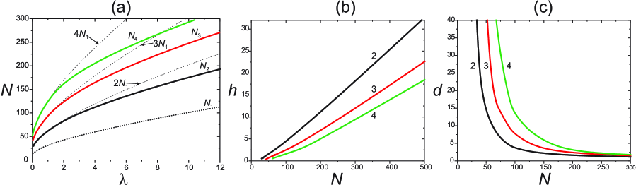
Figure 3: (a) Number of quanta $N$ vs propagation constant $\lambda$. Solid curves for the bound states of $S$ out-of-phase solitons, dashed curves for $SN_{1}$ (variational results). The integers near the curves indicate $S$, the number of solitons.

We next addressed the stability of these multipole solutions and study the evolution (propagation) of the dipoles, tripoles, quadrupoles, and azimuthons in the presence of small initial perturbations. We have undertaken extensive numerical modeling of Eqs. (1) and (2) initialized with our numerically computed multipole solutions with added gaussian noise. The initial condition was taken in the form $\psi(x,y)[1+\varepsilon\Phi(x,y)]$, where $\psi(x,y)$ is the numerically calculated exact multipole solution, $\Phi(x,y)$ is the white gaussian noise with variance $\sigma^{2}=1$ and the parameter of perturbation $\varepsilon=0.005\div 0.1$. Spatial discretization was based on the pseudospectral method and ”temporal” $z$-discretization included the split-step scheme.

Depending on the parameter $\lambda$, we observed three different regimes of the nonrotating dipole propagation, which are presented in Fig. 4 (for $\varepsilon=0.02$). The first regime corresponds to the region $\lambda<\lambda_{cr}$, and we found $\lambda_{cr}\sim 1.9$. If $\lambda<\lambda_{cr}$, the initial dipole splits in two monopoles which move in the opposite directions without changing their shape and without radiation, i. e. the monopoles just go away at infinity. This type of the evolution is shown in Fig. 4(a). The splitting of the dipole into two monopoles can be easily understood. It is seen from Fig. 4 that the bound energy $\delta N=N_{dip}-2N_{mon}$ in the dipole tends to almost zero as $\lambda$ approaches $\lambda_{cr}\sim 1.9$. This explains why the dipole with $\lambda\leq\lambda_{cr}$ can be easily (i. e. under the action of extremely small initial perturbations) split into two monopole-type solitons. A similar behavior, i.e. the decay of the initial dipole into two stable moving monopoles below some critical value of $\lambda$, was observed for the model with a Gaussian response function $R(\xi)$ in Eq. (3) [15].

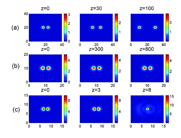
Figure 4: (a) Splitting of the dipole with $\lambda=1.5$ into two monopoles; (b) stable propagation of the dipole with $\lambda=3.5$; (c) unstable dipole with $\lambda=10.$

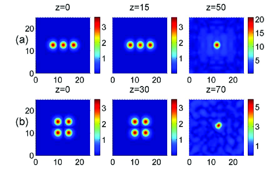
Figure 5: Typical unstable evolution (at $\lambda=2$) of (a) tripole; (b) quadrupole.

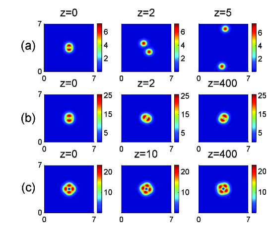
Figure 6: (a) Splitting of the azimuthon with two intensity peaks and $\lambda=10$; (b) stable propagation of the azimuthon with two intensity peaks and $\lambda=80$; (c) stable propagation of the azimuthon with four intensity peaks and $\lambda=80$.

The second regime corresponds to the region $\lambda_{cr}<\lambda<\lambda_{th}$, where $\lambda_{th}\sim 4$. The numerical simulations clearly show that in this range of the parameter $\lambda$ the dipoles are stable with respect to initial noisy perturbations. If the parameter of perturbation $\varepsilon$ is not too large, the dipoles survive over huge distances ($z>3000$). The stable propagation of the dipole is illustrated in Figs. 4(b) (for $\lambda=3.5$ and $\varepsilon=0.02$).

The further (after $\lambda_{th}\sim 4$) increasing the parameter $\lambda$ sharply shortens the propagation distances at which the dipole survives, and, the dipoles with $\lambda>\lambda_{th}$ are unstable. The typical decay of the unstable dipole above the threshold value $\lambda_{th}$ of the rescaled propagation constant is shown in Figs. 4(c). Thus, the stable dipoles exist only within a finite, rather narrow range of the propagation constants $\lambda$.

Figure 5 illustrates the propagation of the tripole and quadrupole for $\lambda=2$, i.e. in the region, where the dipole is stable. Generally speaking, the tripoles and quadrupoles turn out to be unstable, but for $\lambda_{cr}<\lambda<\lambda_{th}$ they can survive on the quite considerable (compared to the characteristic diffraction length) distances and, thus, can be experimentally observed. Tripoles and quadrupoles with $\lambda<\lambda_{cr}$ decay into three and four monopoles respectively.

We observed two different scenarios for the azimuthon propagation. If $\lambda$ (i. e. the beam power) is small enough ($\lambda<15$), the azimuthons are unstable and split into fundamental solitons (monopoles) which move away from each other. An example of such splitting for the azimuthon with two intensity peaks and $\lambda=10$ is presented in Fig. 6(a). For sufficiently large $\lambda$ ($\lambda>15$), the azimuthons turn out to be stable. Stable propagation of the azimuthons with two (rotating dipole) and four (rotating quadrupole) intensity peaks and $\lambda=80$ is shown in Figs. 6(b),(c). Note that stable rotating dipoles were also observed in Ref. [20]. Numerically estimated rotational velocity of the stable azimuthon in Fig. 6(b) is $\omega=1.15$ so that it survives over hundreds rotational periods.

The dynamics of the nonrotating dipole in our model Eqs. (1) and (2) is in sharp contrast to the dipole propagation in the model with a Gaussian response function $R(\xi)$ in Eq. (3), where the stable nonrotating dipoles were observed for all $\lambda>\lambda_{th}$, where $\lambda_{th}$ is some threshold value [14, 15]. A qualitatively different behavior of the dipoles in these models seems to be related to the regularity properties of the functions $R(\xi)$ in Eq. (3) – for the model described by Eqs. (1) and (2) the function $R(\xi)$ has a singularity at zero. The strong dependence of a stability criteria for multisoliton solutions on the regularity properties of the kernel $R$ in Eq. (3) was discussed also in Ref. [15, 20]. The corresponding theoretical problem seems to be intriguing and highly nontrivial.

In conclusion, we have studied the bound states of the out-of-phase nonrotating two-dimensional solitons and rotating multisolitons in nonlocal nonlinear media. We have demonstrated that stationary nonrotating dipolar, tripolar, quadrupolar multisolitons and rotating multisolitons (azimuthons) may exist in media with thermal nonlocal nonlinearity, if the beam power is above some critical value. We have investigated stability of the multisolitons using direct numerical simulations. The nonrotating tripoles and quadrupoles are found to be unstable with respect to decay into fundamental solitons or fusion into single soliton, depending on the beam power. At the same time, we have observed robust propagation of the azimuthons with sufficiently high energy and a dipolar multisoliton with moderate energy. Thus, our theoretical predictions open the prospects for the experimental observations of the stable azimuthons and the bound states of two out-of-phase wave beams in media with thermal self-focusing nonlocal nonlinearity.

References

- [1] C. Conti, M. Peccianti, and G. Assanto, Phys. Rev. Lett. 91 (2003) 073901.
- [2] C. Conti, M. Peccianti, and G. Assanto, Phys. Rev. Lett. 92 (2004) 113902.
- [3] C. Rotschild, O. Cohen, O. Manela, M. Segev, and T. Carmon, Phys. Rev. Lett. 95 (2005) 213904.
- [4] A. G. Litvak, JETP Lett. 4 (1966) 230.
- [5] A. G. Litvak, V. A. Mironov, G. M. Fraiman, and A.D. Yunakovskii, Sov. J. Plasma Phys. 1 (1975) 60 .
- [6] T. A. Davydova and A. I. Fishchuk, Ukr. J. Phys. 40 (1995) 487.
- [7] P. Pedri and L. Santos, Phys. Rev. Lett. 95 (2005) 200404.
- [8] W. Krolikowski, O. Bang, N. I. Nikolov, D. Neshev, J. Wyller, J. J. Rasmussen, and D. Edmundson, J. Opt. B: Quantum Semiclassical Opt. 6 (2004) S288.
- [9] C. Conti, G. Ruocco, and S. Trillo, Phys. Rev. Lett. 95 (2005) 183902.
- [10] See, e.g., Yu. S. Kivshar and G. Agrawal, Optical Solitons: From Fibers to Photonic Crystals (Academic, San Diego, 2003) and references therein.
- [11] A. S. Desyatnikov, A. A. Sukhorukov, and Yu. S. Kivshar, Phys. Rev. Lett. 95 (2005) 203904.
- [12] I. A. Kolchugina, V. A. Mironov, and A. M. Sergeev, Pis’ma Zh. Eksp. Teor. Fiz. 31 (1980) 333 [JETP Lett. 31 (1980) 304].
- [13] V. A. Mironov, A. M. Sergeev, and E. M. Sher, Dokl. Akad. Nauk SSSR 260 (1981) 325 [Sov. Phys. Dokl. 26 (1981) 861].
- [14] S. Lopez-Aguayo et. al., Opt. Letters 31 (2006) 1100.
- [15] A. I. Yakimenko, V. M. Lashkin, and O. O. Prikhodko, Phys. Rev. E 73 (2006) 066605.
- [16] Y.V. Kartashov, V. A. Vysloukh, D. Mihalache and L. Torner, Opt. Letters 31, (2006) 1483.
- [17] C. Rotschild et. al. arXiv:physics/0607039 (2006).
- [18] W. Hu, T. Zhang, Q. Guo, L. Xuan, S. Lan arXiv:physics/0602174 (2006).
- [19] V.I. Petviashvili and V.V. Yan’kov, Rev. Plasma Phys. Vol. 14, Ed. B.B. Kadomtsev, (Consultants Bureau, New York, 1989).
- [20] S. Skupin, O. Bang, D. Edmundson, and W. Krolikowski, Phys. Rev. E 73 (2006) 066603.