Modulated Amplitude Waves in Collisionally Inhomogeneous Bose-Einstein Condensates

Abstract

We investigate the dynamics of an effectively one-dimensional Bose-Einstein condensate (BEC) with scattering length $a$ subjected to a spatially periodic modulation, $a=a(x)=a(x+L)$. This “collisionally inhomogeneous” BEC is described by a Gross-Pitaevskii (GP) equation whose nonlinearity coefficient is a periodic function of $x$. We transform this equation into a GP equation with constant coefficient $a$ and an additional effective potential and study a class of extended wave solutions of the transformed equation. For weak underlying inhomogeneity, the effective potential takes a form resembling a superlattice, and the amplitude dynamics of the solutions of the constant-coefficient GP equation obey a nonlinear generalization of the Ince equation. In the small-amplitude limit, we use averaging to construct analytical solutions for modulated amplitude waves (MAWs), whose stability we subsequently examine using both numerical simulations of the original GP equation and fixed-point computations with the MAWs as numerically exact solutions. We show that “on-site” solutions, whose maxima correspond to maxima of $a(x)$, are significantly more stable than their “off-site” counterparts.

PACS: 05.45.-a, 03.75.Lm, 05.30.Jp, 05.45.Ac

Keywords: Bose-Einstein condensates, periodic potentials, multiple-scale perturbation theory, Hamiltonian systems

I Introduction

Among the most fundamental models studied widely in applied mathematics and employed for the description of an extremely large variety of physical phenomena are nonlinear Schrödinger (NLS) equations sulem . Applications of NLS equations have become even more prominent in recent years due to enormous theoretical and experimental progress that has taken place in studies of Bose-Einstein condensates (BECs) book2 and nonlinear optics book1 . Through the formal similarity between coherent matter waves and electromagnetic waves, research on these topics has become closely connected, and progress in one area frequently also benefits the other. The cross-fertilization between these two fields is extremely important not only from a theoretical perspective but also for applications. For example, coherent matter waves can be manipulated using devices such as atom chips Folman whose design was initially suggested by previously-developed optical counterparts.

In the mean-field approximation, and at sufficiently low temperatures, the dynamics of matter waves are accurately modeled by a cubic NLS equation incorporating an external potential. In this context, it is called the Gross-Pitaevskii (GP) equation book2 ,

$$i\hbar{\Psi}_{t}=\left[-\frac{\hbar^{2}}{2m}\nabla^{2}+\tilde{g}|\Psi|^{2}+{\mathcal{V}}(\vec{r})\right]\Psi\,,$$ (1)

where $m$ is the atomic mass, $\Psi(\vec{r},t)$ is the macroscopic wave function of the condensate, normalized to the number of atoms $N$ (so that $\int|\Psi|^{2}d\mathbf{r}=N$), ${\mathcal{V}}(\vec{r})$ is the external potential, and the effective interaction constant is $\tilde{g}=(4\pi\hbar^{2}a/m)[1+O(\zeta^{2})]$, where $a$ is the s-wave scattering length, and $\zeta^{2}\equiv|\Psi|^{2}|a|^{3}$ measures the density of the atomic gas book2 .

The properties of BECs – including their shape, collective nonlinear excitations (such as solitons and vortices), and fluctuations above the mean-field level – are determined by the sign and magnitude of the scattering length $a$. Accordingly, one of the key tools used in current studies of BECs relies on adjusting $a$ (and hence the nonlinearity coefficient $\tilde{g}$ defined above). A well-known way to achieve this goal is to tune an external magnetic field in the vicinity of a Feshbach resonance Weiner03 ; feshbachNa ; feshbachRb . Alternatively, one can use a Feshbach resonance induced by an optical Theis04 or dc electric electric field. In low-dimensional settings, one can also tune the effective nonlinearity by changing the BEC’s transversal confinement olshani ; Napoli .

Adjusting the scattering length globally (i.e., modifying $a$ in a spatially uniform manner) has been crucial to many experimental achievements, including the formation of molecular condensates molecule and probing the so-called BEC-BCS crossover becbcs . Additionally, recent theoretical studies have predicted that a spatially uniform but time-periodic modulation of the scattering length, with $a(t)$ periodically changing its sign, can be used to stabilize attractive condensates in two FRM1 and three FRMr dimensions and thus help to create robust matter-wave solitons FRM2 . [In the three-dimensional case, the Feshbach resonance-based technique should be combined with a quasi-one-dimensional (quasi-1D) periodic potential, known as an optical lattice (OL).] Other nonlinear waves besides solitons have also been studied in this context. For example, it was predicted that spatially periodic or quasiperiodic 2D patterns resembling the classical Faraday ripples in hydrodynamics can be excited in a BEC via a nonlinear parametric resonance induced by the spatially-uniform and temporally-periodic modulation of $a$ (but, in general, without changing the sign of $a$) Kestutis .

More recently, the possibility of varying the scattering length locally (i.e., spatially) has also been proposed fka ; fermi ; g1 ; v1 . Such spatial dependence of the scattering length, which can be implemented utilizing a spatially inhomogeneous external magnetic field in the vicinity of a Feshbach resonance fermi ; g1 , renders the collisional dynamics inhomogeneous across the BEC. Condensates with a spatially inhomogeneous nonlinearity have recently attracted considerable attention, as they are relevant to many significant applications, including adiabatic compression of matter waves fka ; g1 , Bloch oscillations of matter-wave solitons g1 , atom lasers Peter ; v1 ; v2 , enhancement of transmittivity of matter waves through barriers g2 ; fka2 , and the dynamics of matter waves in the presence of periodic or random spatial variations of the scattering length fka3 . Additionally, while these works chiefly concentrated on quasi-1D condensates, studies in a quasi-two-dimensional (quasi-2D) setting were also recently reported malspace (see also Ref. Gadi for a qualitatively similar model in a different physical context).

In the present work, we consider an effectively one-dimensional BEC whose scattering length is subjected to a periodic variation: $a(x)=a(x+L)$ for some period $L$. We consider the case of no zero crossings, so that $a(x)$ always has the same sign. Such a nonlinear lattice can be realized experimentally (see, e.g., the diagram in Ref. v2 ), and it offers various possibilities for the study of matter-wave solitons (as discussed in Refs. fka3 ; malspace ; fka4 ). Here we focus on the dynamics of spatially extended states (rather than solitons), which have not yet been considered in earlier works in the context of nonlinear lattices. Extended states can be created experimentally, as has been done, for example, in the setting of a BEC in an optical superlattice quasibec .

The analysis of the problem under consideration proceeds as follows. First, we apply a transformation to the quasi-1D GP equation with the nonlinearity coefficient periodically modulated in space in order to derive an effective GP equation with $a=\mathrm{const}$. With this transformation, the original inhomogeneity of $a(x)$ is mapped into an effective linear potential taking the form of a modified superlattice. We consider spatially extended solutions of the transformed GP equation in the form of modulated amplitude waves (MAWs), whose slow-amplitude dynamics we derive using an averaging method. These analytical considerations, presented in Section II, are followed in Section III by an investigation of the dynamics and stability of the MAWs using both direct numerical simulations of the original GP equation and fixed-point computations with the MAWs as numerically exact solutions. We thereby show that “on-site” solutions, whose maxima correspond to maxima of the nonlinear lattice, tend to be more stable than “off-site” solutions. We summarize our findings and present conclusions in Section IV. We then discuss some technical details of the averaging procedure in an appendix (Section V).

II The Perturbed Gross-Pitaevskii Equation

The 3D GP equation (1) can be reduced to an effectively 1D form provided the transverse dimensions of the BEC are on the order of its healing length and its longitudinal dimension is much larger than the transverse ones gp1d ; Napoli . In this regime, the 1D approximation is derived by averaging Eq. (1) in the transverse plane. One can readily show (see, e.g., Ref. g1 ) that the resulting 1D GP equation takes the dimensionless form

$$iu_{t}=-\frac{1}{2}u_{xx}+g(x)|u|^{2}u+V(x)u\,,$$ (2)

where we recall that nonlinearity coefficient $g(x)$ varies in space. In Eq. (2), $u$ is the mean-field wave function (with density $|u|^{2}$ measured in units of the peak 1D density $n_{0}$), $x$ and $t$ are normalized, respectively, to the healing length $\xi=\hbar/\sqrt{n_{0}|g_{1}|m}$ and $\xi/c$ (where $c=\sqrt{n_{0}|g_{1}|/m}$ is the Bogoliubov speed of sound), and energy is measured in units of the chemical potential $\mu=g_{1}n_{0}$. In the above expressions, $g_{1}=2\hbar\omega_{\perp}a_{0}$, where $\omega_{\perp}$ denotes the confining frequency in the transverse direction, and $a_{0}$ is a characteristic (constant) value of the scattering length relatively close to the Feshbach resonance. Finally, $V(x)$ is the rescaled external trapping potential, and the $x$-dependent nonlinearity is given by $g(x)=a(x)/a_{0}$, where $a(x)$ is the spatially varying scattering length.

We will examine periodic modulations of the scattering length by assuming

$$g(x)=g_{0}+V_{0}\sin^{2}(\kappa x)\,,$$ (3)

where $V_{0}$ and $\kappa$ are, respectively, the amplitude and wavenumber of the modulation. In experiments, this modulation mode can be induced by a periodically patterned configuration of the external (magnetic, optical, or electric) field that controls the Feshbach resonance. We chiefly focus on the case of repulsive BECs, with $g_{0}>0$ and $V_{0}>0$. For attractive BECs, for which $g_{0}<0$, one can also transform the nonlinear partial differential equation (2) into an effective GP equation with a constant nonlinearity coefficient.

We now introduce the transformation, $v\equiv\sqrt{g(x)}u$, which casts Eq. (2) in the form

$$iv_{t} = -\frac{1}{2}v_{xx}+|v|^{2}v+V(x)v+\hat{V}_{\mathrm{eff}}(x)v\,,$$

$$\hat{V}_{\mathrm{eff}}(x) = \frac{1}{2}\frac{f^{\prime\prime}}{f}-\frac{\left(f^{{}^{\prime}}\right)^{2}}{f^{2}}+\frac{f^{\prime}}{f}\frac{\partial}{\partial x}\,,$$ (4)

where $f(x)\equiv\sqrt{g(x)}$, and $f^{\prime}\equiv df/dx$. Obviously, this transformation applies only in the case when $g(x)$ does not cross zero.

If the scattering-length modulation is weak, i.e., $V_{0}\ll g_{0}$ in Eq. (3), then $\hat{V}_{\mathrm{eff}}$ can be approximated as a superlattice potential (because it contains a second harmonic in addition to the fundamental one) plus a first-derivative operator term:

$$\hat{V}_{\mathrm{eff}}(x)=-\frac{3\kappa^{2}V_{0}^{2}}{16g_{0}^{2}}+\frac{\kappa^{2}V_{0}}{2g_{0}}\cos(2\kappa x)+\frac{3\kappa^{2}V_{0}^{2}}{16g_{0}^{2}}\cos(4\kappa x)+\left[\frac{V_{0}\kappa}{2g_{0}}\sin(2\kappa x)\right]\frac{\partial}{\partial x}\,.$$ (5)

In this case, we define a small parameter, $\varepsilon\equiv\kappa V_{0}/g_{0}$, evincing the fact that the $\cos(4\kappa x)$ harmonic in Eq. (5) is a small correction to the fundamental one, $\cos(2\kappa x)$. Thus, to order $O(\epsilon)$, the effective potential (5) is a modified lattice rather than a superlattice.

It is also worth mentionioning that in the case of a temporal modulation of the scattering length, i.e., $g=g(t)$ in Eq. (2), the same transformation defined above can be used (i.e., $v\equiv\sqrt{g(t)}u$) provided $g(t)$ never vanishes. As is well known, the time-dependent coefficient in front of the nonlinear term is then translated into a linear dissipative term on the right-hand side of the equation for $v(x,t)$ Manakov . This term has the time-dependent coefficient $-i(2g)^{-1}(dg/dt)v$. While this latter setting may be of interest in its own right (perhaps especially when the dissipation coefficient is constant so that the time dependence can be completely factored out – i.e., for $g(t)$ of an exponential form), we do not pursue it further here. We remark that if $g(t)$ is a periodic function, the transformed equation will generate patterns with a periodically oscillating amplitude. Finally, one can complicate the situation still further by considering simultaneous spatial and temporal modulations [i.e., $g=g(x,t)$], though such a configuration would be very difficult to controllably implement in experiments.

III Modulated Amplitude Waves

We consider solutions to Eqs. (4,5) in the form of coherent structures given by the ansatz

$$v(x,t)=R(x)\exp\left(i\left[\theta(x)-\mu t\right]\right)\,.$$ (6)

Such nonlinear waves, called modulated amplitude waves (MAWs), have been studied previously in BEC models with optical-lattice and superlattice potentials map1 ; map2 ; map3 ; map4 . Because of the spatial periodicity of the potential in Eq. (4), MAWs in the linear limit yield the particular case of Bloch waves (of the transformed GP equation). Generic Bloch wave functions are quasiperiodic in $x$; periodic ones lie at edges of Bloch bands.

Inserting Eq. (6) into Eq. (4) and equating the real and imaginary components of the resulting equation yields an ordinary differential equation governing the spatial amplitude dynamics. For standing waves (for which $\theta(x)=0$), this equation is

$$\frac{d^{2}R}{dx^{2}}-\varepsilon\frac{dR}{dx}\sin(2\kappa x)+\left[2\tilde{\mu}-\varepsilon\kappa\cos(2\kappa x)-\frac{3}{8}\varepsilon^{2}\cos(4\kappa x)-2V(x)\right]R-2R^{3}=0\,,$$ (7)

where $2\tilde{\mu}=2\mu+(3/8)\varepsilon^{2}$. Equation (7), known as a nonlinear generalized Ince equation ngince , is reminiscent of the nonlinear Mathieu equation, but with the parametric force acting on both $R$ and $R^{\prime}$. In the linear limit, one can study Bloch waves by applying Floquet theory to Eq. (7). In particular, one can employ the method of harmonic balance 675 , in which one inserts a Fourier series expansion into the (linear) generalized Ince equation and studies the resulting infinite set of coupled linear algebraic equations satisfied by the Fourier coefficients.

III.1 Small-Amplitude Solutions

Let us now consider Eq. (7) in the absence of the external trapping potential $V(x)$. As shown by Eqs. (4) and (5), the effective superlattice potential $\hat{V}_{\mathrm{eff}}(x)$ is already a confining potential for the condensate. Seeking small-amplitude solutions, we employ the scaling $R\equiv\sqrt{\varepsilon/2}s$, which transforms Eq. (7) into

$$\frac{d^{2}s}{dx^{2}}-\varepsilon\sin(2\kappa x)\frac{ds}{dx}+\left[\delta^{2}-\varepsilon\kappa\cos(2\kappa x)-\frac{3}{8}\varepsilon^{2}\cos(4\kappa x)\right]s-\varepsilon s^{3}=0\,,$$ (8)

where $\delta^{2}\equiv 2\tilde{\mu}$ (implying that $\tilde{\mu}$ is positive). The alternative scaling $R\equiv\varepsilon w/\sqrt{2}$ would produce a nonlinearity of size $O(\varepsilon^{2})$ rather than $O(\varepsilon)$ in Eq. (8) and would lead one even deeper into the small-amplitude regime.

Equation (8) is of the form

$$s^{\prime\prime}+\delta^{2}s=\varepsilon F_{1}(s,s^{\prime},x)+\varepsilon^{2}F_{2}(s,s^{\prime},x)\,,$$ (9)

where

$$F_{1}(s,s^{\prime},x) \equiv\kappa s\cos(2\kappa x)+s^{\prime}\sin(2\kappa x)+s^{3}\,,$$

$$F_{2}(s,s^{\prime},x) \equiv\frac{3s}{8}\cos(4\kappa x)\,.$$ (10)

As in Ref. map4 , we consider situations near the 2:1 subharmonic resonance, for which $\delta=\pm\kappa$ in Eq. (9). Assuming a small “detuning” from the exact resonance, we introduce the expansion

$$\delta=\kappa+\varepsilon\delta_{1}+\varepsilon^{2}\delta_{2}+O(\varepsilon^{3})\,,$$ (11)

which we insert in Eq. (9) to obtain

$$s^{\prime\prime}+\kappa^{2}s=\varepsilon G_{1}(s,s^{\prime},x)+\varepsilon^{2}G_{2}(s,s^{\prime},x)+O\left(\varepsilon^{3}\right)\,,$$ (12)

where

$$G_{1}(s,s^{\prime},x) \equiv-2\delta_{1}\kappa s+F_{1}(s,s^{\prime},x)\,,$$

$$G_{2}(s,s^{\prime},x) \equiv\left(-\delta_{1}^{2}-2\delta_{2}\kappa)s+F_{2}(s,s^{\prime},x\right)\,.$$ (13)

When $\varepsilon=0$, Eq. (12) has the solution

$$s=\rho\cos(\kappa x+\phi)\,,$$ (14)

with first derivative $s^{\prime}=-\kappa\rho\sin(\kappa x+\phi)$. We now use the solution (14) and its derivative as a starting point to apply the method of variation of parameters to equation (12). We therefore seek a solution to Eq. (12) of the form

$$s(x)=\rho(x)\cos(\kappa x+\phi(x))\,,\quad s^{\prime}(x)=-\kappa\rho(x)\sin(\kappa x+\phi(x))\,,$$ (15)

where $\rho(x)$ and $\phi(x)$ are slowly varying functions. Differentiating the expression for $s(x)$ in Eq. (15), we enforce the following consistency condition with the expression for $s^{\prime}(x)$ in (15):

$$\rho^{\prime}\cos(\kappa x+\phi)=\rho\phi^{\prime}\sin(\kappa x+\phi)\,.$$ (16)

Subsequently inserting the result in Eq. (12) yields

$$\rho^{\prime}= - \frac{\varepsilon}{\kappa}\sin(\kappa x+\phi)G_{1}\left(\rho\cos(\kappa x+\phi),-\kappa\rho\sin(\kappa x+\phi),x\right)$$ (17)

$$- \frac{\varepsilon^{2}}{\kappa}\sin(\kappa x+\phi)G_{2}\left(\rho\cos(\kappa x+\phi),-\kappa\rho\sin(\kappa x+\phi),x\right)\,,$$

$$\phi^{\prime}= - \frac{\varepsilon}{\kappa\rho}\cos(\kappa x+\phi)G_{1}\left(\rho\cos(\kappa x+\phi),-\kappa\rho\sin(\kappa x+\phi),x\right)$$ (18)

$$- \frac{\varepsilon^{2}}{\kappa\rho}\cos(\kappa x+\phi)G_{2}\left(\rho\cos(\kappa x+\phi),-\kappa\rho\sin(\kappa x+\phi),x\right)\,.$$

Our objective is to isolate the components of $\rho(x)$ and $\phi(x)$ that vary slowly as compared to the fast oscillations of $\cos(\kappa x)$ and $\sin(\kappa x)$ and to derive averaged equations governing the dynamics of these parts. To commence averaging, we decompose $\rho$ and $\phi$ into a sum of the slowly varying parts and small, rapidly oscillating corrections. That is,

$$\rho =c+\varepsilon w_{1}(c,\varphi,x)+\varepsilon^{2}v_{1}(c,\varphi,x)+O(\varepsilon^{3})\,,$$

$$\phi =\varphi+\varepsilon w_{2}(c,\varphi,x)+\varepsilon^{2}v_{2}(c,\varphi,x)+O(\varepsilon^{3})\,.$$ (19)

We then substitute Eqs. (19) into Eqs. (17)-(18) and Taylor-expand to obtain

$$c^{\prime} = \varepsilon\left[-\frac{\partial w_{1}}{\partial x}-\frac{1}{\kappa}\sin(\kappa x+\varphi)G_{1}(c\cos(\kappa x+\varphi),-\kappa c\sin(\kappa x+\varphi),x)\right]$$ (20)

$$+ \varepsilon^{2}\left[-\frac{\partial v_{1}}{\partial x}+L_{1}(c,\varphi,x)\right]+O(\varepsilon^{3})\,,$$

$$\varphi^{\prime} = \varepsilon\left[-\frac{\partial w_{2}}{\partial x}-\frac{1}{\kappa c}\cos(\kappa x+\varphi)G_{1}(c\cos(\kappa x+\varphi),-\kappa c\sin(\kappa x+\varphi),x)\right]$$ (21)

$$+ \varepsilon^{2}\left[-\frac{\partial v_{2}}{\partial x}+L_{2}(c,\varphi,x)\right]+O(\varepsilon^{3})\,.$$

The functions $w_{1}$ and $w_{2}$ in Eqs. (19)-(21) should be chosen so as to eliminate all the rapidly oscillating terms at order $O(\varepsilon)$. At $O(\varepsilon^{2})$, the functions $v_{1}$ and $v_{2}$ are similarly chosen. The terms $L_{1}(c,\varphi,x)$ and $L_{2}(c,\varphi,x)$ in Eqs. (20)-(21) depend on $w_{1}$, $w_{2}$, $G_{1}$, and $G_{2}$. We provide expressions for $w_{1}$, $w_{2}$ and $L_{1}$, $L_{2}$ in the Appendix. (Note that expressions for $v_{1}(x)$ and $v_{2}(x)$ are not needed until one tackles the third-order corrections, so we do not display them.) The functions $G_{1}$ and $G_{2}$ are expressed in terms of $c$ and $\varphi$ as follows:

$$G_{1}(c,\varphi,x) =-2\delta_{1}\kappa c\cos(\kappa x+\varphi)+\kappa c\cos(\kappa x+\varphi)\cos(2\kappa x)$$

$$-\kappa c\sin(\kappa x+\varphi)\sin(2\kappa x)+c^{3}\cos^{3}(\kappa x+\varphi)\,,$$

$$G_{2}(c,\varphi,x) =\left(-\delta_{1}^{2}-2\delta_{2}\kappa\right)c\cos(\kappa x+\varphi)+\frac{3}{8}c\cos(\kappa x+\varphi)\cos(4\kappa x)\,.$$

To first order, the slow evolution equations are

$$c^{\prime}=O\left(\varepsilon^{2}\right)\,,~{}\varphi^{\prime}=\varepsilon\left(\delta_{1}-\frac{3c^{2}}{8\kappa}\right)+O(\varepsilon^{2})\,,$$ (22)

generating a circle of nonzero equilibria with amplitude $c_{\ast}=\sqrt{8\delta_{1}\kappa/3}$. The generating functions $w_{1}(x)$ and $w_{2}(x)$ that yield these equations are shown in the Appendix. This process results in the amplitude function

$$R(x)=\sqrt{\frac{\varepsilon}{2}}c_{\ast}\cos(\kappa x+\varphi_{\ast})\equiv v(x,t=0)\,,$$ (23)

where the phase shift $\varphi_{\ast}$ is arbitrary. The corresponding MAW is given by $v(x,t)=R(x)\exp(-i\mu t)$, as per Eq. (6).

Returning to the original GP equation (in the absence of an external potential), we obtain the MAW $u(x,t)=v(x,t)/\sqrt{g(x,t)}$. We examine its dynamics and stability with direct simulations of Eq. (2) with $V(x)=0$. Results of the simulations for $g_{0}=2$, $V_{0}=0.15$, $\kappa=\pi/8$ (so that $\varepsilon\approx 0.0295$), $\delta_{1}=3$, $\delta_{2}=1$, and $\varphi_{\ast}=0$ are shown in Fig. 1. These parameter values correspond to a ⁸⁷Rb (or a ²³Na) condensate in a trap with transverse confining frequency $\omega_{\perp}=2\pi\times 1000$Hz that contains $N\approx 10^{3}$ atoms with a peak 1D density $n_{0}=10^{8}$ m^-1. Here, the spatial unit (i.e., the healing length) is $\xi=0.3\,\mu$m ($\xi=0.9\,\mu$m), and the temporal unit is $\xi/c=0.14$ ms ($\xi/c=0.3$ ms). Figure  1 shows that the MAW appears to be stable for long times as a solution of the original GP equation. For larger $\varepsilon$, however, the wave breaks up into solitary filaments (that appear to be localized around the maxima of the nonlinear optical lattice; see the discussion below), as indicated in Fig. 2 (for $V_{0}=1.5$). In fact, as we will discuss below, the apparently stable MAWs obtained for small $V_{0}$ are actually weakly unstable, although their lifetimes are very long. The normalized time $t=2000$ amounts to $280$ ms for a Rubidium (and $600$ ms for a Sodium) BEC in real time, suggesting that these MAWs can nevertheless be observed in experiments.

  

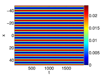
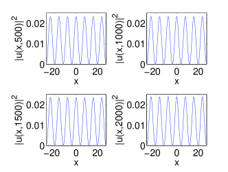
Figure 1: (Color online) Dynamical evolution of the sinusoidal MAW of Eq. (23) with parameter values $\phi_{\star}=0$ for $g_{0}=2$, $\kappa=\pi/8$, $V_{0}=0.15$, $\delta_{1}=3$, and $\delta_{2}=1$. The left panel shows the space-time contour plot of the square modulus (density) $|u|^{2}$ of the solution, and the right panels show four snapshots (spatial profiles) of the spatio-temporal evolution. The dynamics illustrate an apparent stability of the solution up through at least $t=2000$.

  

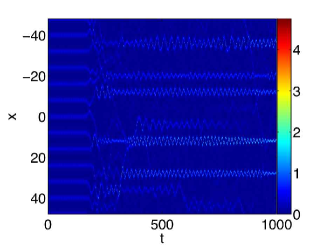
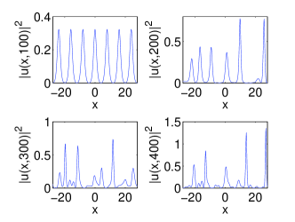
Figure 2: (Color online) Same as Fig. 1, but for $V_{0}=1.5$. As early as $t=200$, the MAW solution starts breaking up into solitary filaments that appear to be localized around the maxima of the nonlinear optical lattice (see the discussion in the text).

  

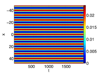
Figure 3: (Color online) Same as Fig. 1 (and also with $V_{0}=0.15$), but for the refined prediction of the initial MAW solution based on Eq. (24). The solution also appears to be dynamically stable.

  

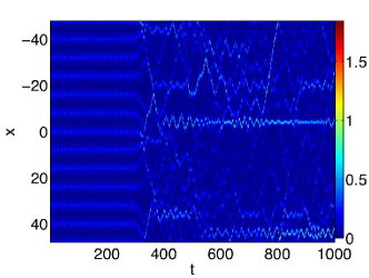
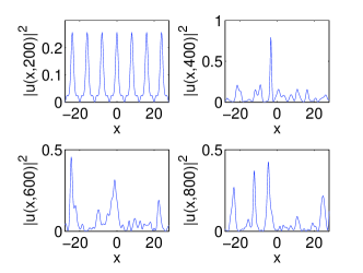
Figure 4: (Color online) Same as Fig. 2, but with the MAW of Eq. (24) used as the initial condition for the time-evolution of the GP equation. Observe that the refined initial condition leads to a delayed initiation of the instability (which now begins at about $t\approx 300$).

One can also incorporate the generating functions into the MAWs and examine the stability properties of the resulting refined MAWs using direct numerical simulations. These MAWs are given by

$$R(x)=\sqrt{\frac{\varepsilon}{2}}(c_{\ast}+\varepsilon w_{1})\cos(\kappa x+\varphi_{\ast}+\varepsilon w_{2})\equiv v(x,t=0)$$ (24)

instead of Eq. (23). We plot the corresponding space-time plots and spatial profiles at various time instants for $V_{0}=0.15$ in Fig. 3 and for $V_{0}=1.5$ in Fig. 4. All other parameters are the same as before. It is readily observed that the instability in Fig. 4 sets in later (at $t\approx 300$) than that in Fig. 2 (at $t\approx 200$), which was obtained with the same parameter values using the sinusoidal MAW of Eq. (23).

The MAWs in Eqs. (23) and (24) were determined to order $O(\varepsilon)$, so they ignore the effects of the second-harmonic component of the lattice, which arise at $O(\varepsilon^{2})$. To estimate the influence of this component, we used the same MAWs as initial conditions in direct simulations of the original GP equations in the presence of an additional external optical lattice (OL) potential, $V(x)=-(3/16)\varepsilon^{2}\cos(4\kappa x)$ that exactly cancels out the second-harmonic component of the lattice. While differences between the results of the simulations with and without the compensating OL are not apparent in comparing space-time plots side-by-side, one can observe the slow development of small discrepancies by examining the time-evolution of the absolute value of their difference.

To second order, the equations of slow evolution are

$$c^{\prime} =\varepsilon^{2}\left[\frac{c}{4\kappa}\left(\delta_{1}-\frac{c^{2}}{8\kappa}\right)\sin(2\varphi)\right]+O(\varepsilon^{3})\,,$$

$$\varphi^{\prime} =\varepsilon\left(\delta_{1}-\frac{3c^{2}}{8\kappa}\right)+\varepsilon^{2}\left[\delta_{2}-\frac{1}{16\kappa}+\frac{3c^{2}\delta_{1}}{4\kappa^{2}}-\frac{51c^{4}}{256\kappa^{3}}+\frac{1}{4\kappa}\left(\delta_{1}-\frac{c^{2}}{4\kappa}\right)\cos(2\varphi)\right]+O(\varepsilon^{3})\,.$$ (25)

In contrast to the first-order equations (22), the equilibrium points of Eqs. (25) depend on $\varepsilon$, which is typical in second-order averaging. In studying the dynamics of slow-flow equations produced by such a procedure, one obtains, in general, a complicated bifurcation problem, which can be investigated by taking $\varepsilon$ small but fixed (see, e.g., Ref. ngmat ). For our purposes, we simply note that the only difference between Eqs. (25) and the slow equations one would obtain at second order without the $O(\varepsilon^{2})$ lattice term in Eq. (7) amounts to constant terms at the same order [they result directly from the detuning of $\delta$; see Eq. (11)]. Without the second-order lattice term, $\delta_{2}$ would not be present, and there would be an additional constant term, $-\delta_{1}^{2}/(2\kappa)$, that is cancelled out here because of the extra harmonic. To study the effects of the second-order lattice systematically, one can examine the dynamics starting with the alternative scaling $R\equiv\varepsilon w/\sqrt{2}$ (rather than $R\equiv\sqrt{\varepsilon/2}s$, as adopted above), in which case the effect of the nonlinearity also emerges at second order.

In the absence of resonances, second-order averaging yields slow dynamical equations for $(c,\varphi)$ with $c^{\prime}=O\left(\varepsilon^{3}\right)$ and $\varphi^{\prime}<0$, so that a fixed-radius circle is traversed in the clockwise direction. From here, one can also consider resonances whose effects appear at $O(\varepsilon^{2})$.

III.2 Stability

In Figs. 2 and 4, we observe that the MAW initial conditions, derived for small $V_{0}$, break down rather quickly for larger $V_{0}$. In fact, there is a weak instability even for small $V_{0}$, although the time it takes for the instability to set in is rather long (beyond $t=2000$). Thus, the MAW solutions have a good chance to be observed experimentally for sufficiently small scattering-length modulations $V_{0}$. (Recall that $t=2000$ corresponds to $280$ ms for a ⁸⁷Rb BEC and $600$ ms for a ²³Na one.)

To investigate this point further, we performed fixed-point computations using Eqs. (23) and (24) as starting guesses in order to obtain numerically exact stationary states. We show the results for Eq. (23) in Fig. 5 using a computational domain containing one period of the solution. In this context, we have implemented a variant of our finite-difference method (for the spatial discretization) that incorporates Floquet theory, as is described in, e.g., bernard . Adding an $\exp(i\theta)$ term and its complex conjugate at the appropriate locations of our stability matrix, we fill in the bands of continuous spectrum by varying $\theta$ within the interval $[0,2\pi)$. We used a partition of $200$ equidistant points in $\theta$ for the results shown here. We find that the configuration is always unstable, even for the small $V_{0}$ that appeared to be stable based on direct numerical simulations. Hence, the apparent stability of Figs. 1 and 3 arises only because of the fact that the simulation was performed for a finite time (up to $t=2000$). As indicated in Fig. 5 (where the spectral planes are plotted in the bottom panels), the instability is weak for small $V_{0}$ but becomes strong for large $V_{0}$.

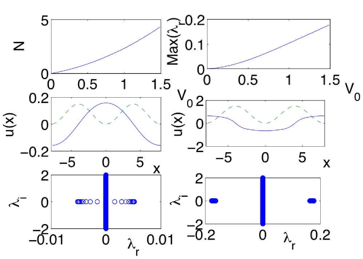
Figure 5: (Color online) Results of a fixed point iteration to identify the solution given by Eq. (23) as a numerically exact stationary state. The top left panel shows the $L^{2}$ norm (density) of this state in our computational domain (containing one period of the solution), and the top right panel shows the maximal real part of the most unstable eigenvalue of the configuration. Observe that the configuration is always unstable. Hence, the apparent stability of Figs. 1 and 3 arises only because of the finite time (up to $t=2000$) of the direct GP simulations. The middle left and right panels show the solution (solid curve) and nonlinear lattice $g(x)$ (dashed curve) for $V_{0}=0.15$ and $V_{0}=1.5$, respectively. The bottom left and right panels show the corresponding spectral planes of the solutions and indicate the weak instability of the former and the strong instability of the latter.

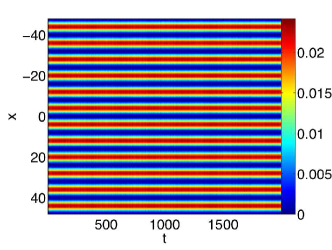
(a)    (b)

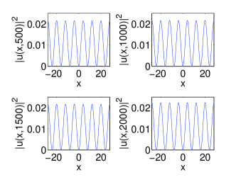
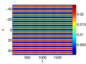
(c)    (d)

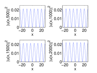
Figure 6: (Color online) Dynamical evolution of the on-site solutions with $\phi_{\star}=\pi/2$ for the initial waves of Eq. (23) [panels (a) and (b)] and Eq. (24) [panels (c) and (d)]. In both cases, $V_{0}=0.15$.

To find more stable solutions, we note that the transformation $v\equiv\sqrt{g(x)}u$ suggests that for the nonlinear OL, solutions prefer to be centered on-site (in contrast to what occurs for linear OLs), so that their maxima coincide with maxima of the lattice rather than minima. This is not surprising, as the multiplicative terms (i.e., the ones without the $d/dx$) of $V_{\mathrm{eff}}(x)$ act as a regular (super)lattice after the transformation and the minima of $g(x)$ coincide with the maxima of these terms in $V_{\mathrm{eff}}(x)$. (We note in passing that this difference between linear and nonlinear OLs has also recently been highlighted in wein06 from a spectral theory perspective for bright soliton solutions of the NLS equation.) We observe additionally in Figs. 2 and 4 that when the MAWs break up, one obtains solutions that are localized on maxima of the nonlinear OL. We can take advantage of this observation by using MAWs with different phases $\varphi_{\ast}$ as initial wave functions in simulations of the GP equation (2).

We show the dynamical evolution of on-site MAWs (for which $\varphi_{*}=\pi/2$) in Figs. 6 and 7 for $V_{0}=0.15$ and $V_{0}=1.5$, respectively. As observed in Fig. 7, the solution remains stable past $t=1000$ instead of breaking up far earlier, as was the case for off-site solutions. We confirm these observations on stability using fixed-point computations of the same type as above (but now for solutions with $\varphi_{*}=\pi/2$), the results of which are shown in Fig. 8. We observe that the maximum eigenvalue now has a much smaller value and that the ensuing instabilities here are much weaker oscillatory ones. An interesting feature that we note in passing is the formation of “rings” of such oscillatory instabilities (see Fig. 8).

The stability results discussed above can also be considered in light of the recent work zoilong on the development of instabilities for NLS equations with constant nonlinearity coefficients and periodic potentials. The authors of Ref. zoilong found (among other results) that small-amplitude, periodic, standing-wave solutions corresponding to band edges alternate in their stability, where upper band edges are modulationally unstable in the attractive case and lower band edges are modulationally unstable in the repulsive case. The theory in zoilong is also applicable to the MAW solutions constructed above, as the resonance relation they satisfy guarantees their spatial periodicity.

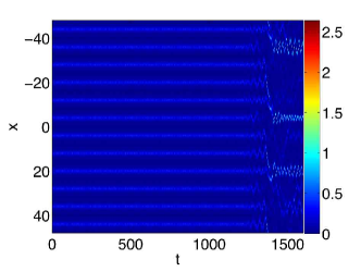
(a)    (b)

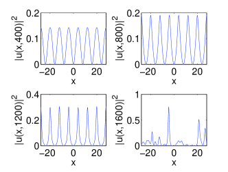
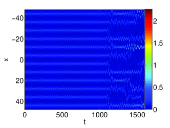
(c)    (d)

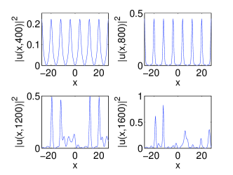
Figure 7: (Color online) Same as Fig. 6, except for $V_{0}=1.5$. Observe that the solutions now become unstable for times longer than $t=1000$, highlighting the much weaker nature of the corresponding instability in comparison to its off-site counterpart. The fact that the refined ansatz (24) now seems to become unstable at an earlier time is probably due to the significant change in the profile of the (exact) solution for large $V_{0}$ (see Fig. 8).

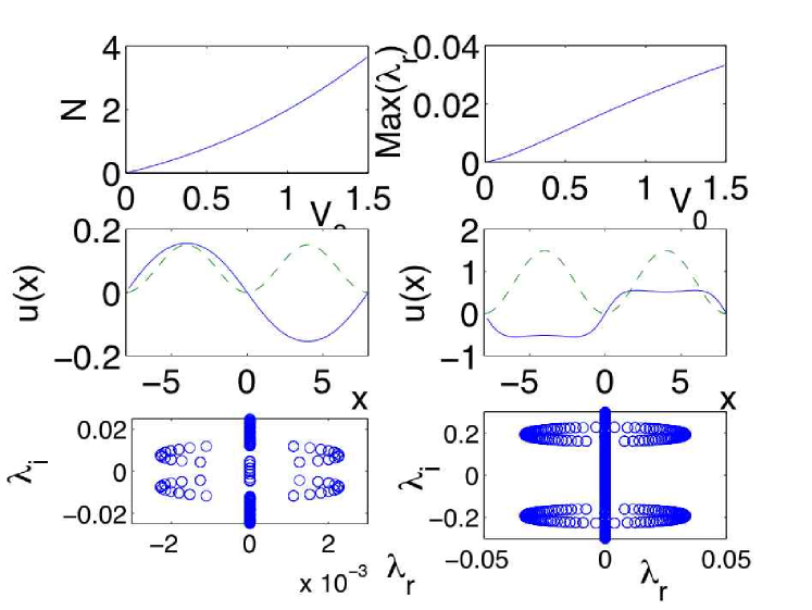
Figure 8: (Color online) Same as Fig. 5, except for on-site MAWs. In this case, the instability of the solutions is much weaker and is oscillatory in nature.

To examine the onset of modulational instabilities, we consider small perturbations to the MAWs of the form $u_{1}\exp(\lambda t-i\mu t)$. [That is, one linearizes the GP equation (2) around the MAW solutions.] Such perturbations satisfy the Bogoliubov equations,

$$L_{+}p=\lambda q\,,\quad L_{-}q=\lambda p\,,$$ (26)

where the amplitude $u_{1}=p+iq$ and

$$L_{-} =-\frac{1}{2}\frac{d^{2}}{dx^{2}}+V(x)+g(x)|u_{MAW}|^{2}-\mu\,,$$

$$L_{+} =-\frac{1}{2}\frac{d^{2}}{dx^{2}}+V(x)+3g(x)|u_{MAW}|^{2}-\mu\,.$$ (27)

Recall that in the absence of a linear optical lattice, $V(x)\equiv 0$.

In Ref. zoilong , it is shown that a sufficient condition for the onset of the modulational instability is for $\lambda=0$ to be in the interior of a band of the $L_{+}$ operator. When $\lambda=0$, Eqs. (27) decouple, so that $L_{+}p=L_{-}q=0$. With the sinusoidal solution (23), we obtain the following Mathieu equations for $V(x)=0$:

$$-\frac{1}{2}\frac{d^{2}q}{dx^{2}}+\left[\left(\frac{\varepsilon c_{*}^{2}}{4}-\mu\right)+\frac{\varepsilon c_{*}^{2}}{4}\cos(2\kappa x+2\varphi_{*})\right]q =0\,,$$

$$-\frac{1}{2}\frac{d^{2}p}{dx^{2}}+\left[\left(\frac{3\varepsilon c_{*}^{2}}{4}-\mu\right)+\frac{3\varepsilon c_{*}^{2}}{4}\cos(2\kappa x+2\varphi_{*})\right]p =0\,,$$ (28)

where we recall that $2\tilde{\mu}=2\mu+(3/8)\varepsilon^{2}=\kappa^{2}$, $c_{\ast}=\sqrt{8\delta_{1}\kappa/3}$, and $\delta_{1}$ and $\varphi_{*}$ are free parameters. (Note that the factors of $g(x)$ in (27) cancel out with $g(x)$ factors in $|u_{MAW}|^{2}$ because of the transformation used to construct the MAW solutions.) In the Mathieu equation $L_{+}p=0$, the parameter combinations are $3\varepsilon c_{*}^{2}/4=2\varepsilon\delta_{1}\kappa$ and $\mu=\kappa^{2}/2-3\varepsilon^{2}/16$. In the limit $\varepsilon\longrightarrow 0$ (i.e., $V_{0}\longrightarrow 0$), equations (28) become linear harmonic oscillators.

To examine the applicability of the aforementioned theorem of zoilong in the present setting, we have computed the eigenvalues of $L_{+}$. In particular, as a systematic measure for the inclusion of the zero eigenvalue in a band of eigenvalues of $L_{+}$, we consider $\min\left\{|\lambda_{L_{+}}|\right\}$, where $\lambda_{L_{+}}$ denotes the eigenvalues of the operator. We show this diagnostic in Fig. 9 for solutions with $\phi_{\star}=0$. One can see that for $V_{0}<0.5$ (roughly), the $0$ eigenvalue is, within the levels of our numerical accuracy, contained in a band of $L_{+}$. This, according to the results of zoilong , implies the existence of modulational instability in this case. On the other hand, for larger $V_{0}$, this no longer occurs. However, because the criterion only offers a sufficient condition, the results are inconclusive in this latter case. Nevertheless, the full numerical results of Fig. 5 indicate the presence of instability here as well. For $\phi_{\star}=\pi/2$, we do not find the $0$ eigenvalue remaining in a band of the $L_{+}$ eigenvalues for increasing $V_{0}$. Hence, for that case as well, we need to revert to the full numerical results of Fig. 8.

One can also examine the sufficient condition of zoilong from a theoretical perspective using properties of Hill’s equations. The eigenvalue problem $L_{+}p=\lambda_{L_{+}}p$ is described by the Mathieu equation

$$\frac{d^{2}p}{d\chi^{2}}+\left[\alpha+2\beta\cos(2\chi+2\phi_{*})\right]p=0\,,$$ (29)

where $\chi=\kappa x$ and

$$\alpha=1+\frac{2\lambda_{L_{+}}}{\kappa^{2}}-\frac{4\varepsilon\delta_{1}}{\kappa}-\frac{3\varepsilon^{2}}{8\kappa^{2}}\,,\quad\beta=-\frac{2\varepsilon\delta_{1}}{\kappa}\,.$$ (30)

From Floquet theory, we construct solutions to (29) of the form $p(\chi)=\exp(\gamma(\lambda_{L_{+}})\chi)Z(\chi)$, where $Z(\chi)$ is a periodic function with period $\pi$ and $\gamma(\lambda_{L_{+}})$ is known as the characteristic (or Floquet) exponent ince ; nayfeh .

Expanding $Z(\chi)$ in a Fourier series and equating each of its coefficients to zero yields an infinite-dimensional matrix, whose determinant $\Delta(\gamma)$ (the so-called “Hill determinant”) is given by

$$\Delta(\gamma)=\Delta(0)-\frac{\sin^{2}\left[\frac{1}{2}i\pi\gamma\right]}{\sin^{2}\left[\frac{1}{2}\pi\sqrt{\alpha}\right]}\,.$$ (31)

The Floquet exponents satisfy $\Delta(\gamma)=0$, so they are given by ince ; nayfeh

$$\gamma=\pm\frac{2i}{\pi}\sin^{-1}\left\{\left[\Delta(0)\sin^{2}\left(\frac{1}{2}\pi\sqrt{\alpha}\right)\right]^{1/2}\right\}\,.$$ (32)

To determine the spectral bands, one then computes the trace of the fundamental matrix of (29), which is given by pel

$$\mathrm{tr}_{M}(\lambda_{L_{+}})=2\cos\left[-i\pi\gamma(\lambda_{L_{+}})\right]\,.$$ (33)

The spectral bands of (29) are defined by the condition $|\mathrm{tr}_{M}(\lambda_{L_{+}})|\leq 2$.

Computing $\Delta(0)$ is, in general, nontrivial, but it is permissible to consider a finite-dimensional truncation of the (center of the) Hill matrix provided $\beta$ is small. Using the example $\varphi_{*}=0$, the five-dimensional truncation of the matrix is given by

$$\begin{pmatrix}1&\frac{\beta}{\alpha-16}&0&0&0\\ \frac{\beta}{\alpha-4}&1&\frac{\beta}{\alpha-4}&0&0\\ 0&\frac{\beta}{\alpha}&1&\frac{\beta}{\alpha}&0\\ 0&0&\frac{\beta}{\alpha-4}&1&\frac{\beta}{\alpha-4}\\ 0&0&0&\frac{\beta}{\alpha-16}&1\end{pmatrix}\,.$$

With the parameter values $\kappa=\pi/8$, $V_{0}=0.15$, $g=2$, and $\delta_{1}=1$ (for which $\beta=0.15$), we obtain the plot of $\mathrm{tr}_{M}(\lambda_{L_{+}})$ shown in Fig. 10. The eigenvalue $\lambda_{L_{+}}=0$ is part of the band, indicating that a modulational instability occurs. While this semi-analytical approach is presented for completeness and is of interest in its own right, its use of a truncated Hill matrix and of an approximate analytical solution seems to indicate that it is preferable to follow the diagnostic of Fig. 9 presented above.

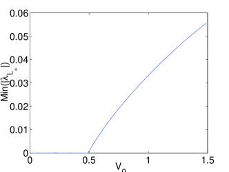
Figure 9: The minimal-magnitude eigenvalue of $L_{+}$ as a function of $V_{0}$ for $\phi_{\star}=0$ solutions. The $0$ value of this diagnostic indicates the presence of modulational instability.

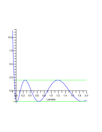
Figure 10: (Color online) Trace of the fundamental matrix (vertical axis) versus eigenvalue $\lambda_{L_{+}}$ of the $L_{+}$ operator. One obtains spectral bands when the magnitude of the trace is bounded by 2. The zero eigenvalue occurs within such a band, indicating that there is a modulational instability. The right panel shows a magnification of the left panel.

IV Conclusions

In this paper, we have investigated the existence and stability of modulated amplitude waves (MAWs) in quasi-one-dimensional Bose-Einstein condensates (BECs) in “nonlinear lattices”. In particular, we considered an experimentally feasible situation in which the condensate’s $s$-wave scattering length is modulated periodically in space. Accordingly, we analyzed the Gross-Pitaevskii (GP) equation with a spatially periodic nonlinearity coefficient. We transformed this GP equation into a new GP equation with a constant nonlinearity coefficient and (for small modulations of the scattering length) an effective (quasi-)superlattice potential. We subsequently studied spatially extended solutions by applying a coherent-structure ansatz to the latter equation, which leads to a nonlinear generalized Ince equation governing the amplitude’s spatial dynamics. In the small-amplitude limit, we used averaging to construct MAW solutions, whose stability we examined using both direct numerical simulations of the original GP equation and fixed-point computations with the MAWs as numerically exact solutions.

While direct simulations suggest stability of the constructed MAW solutions for sufficiently weak periodic modulations, the fixed-point computations indicate that even those are weakly unstable (though they can persist long enough to permit experimental observations) for “off-site” solutions, whose maxima do not coincide with maxima of the nonlinear lattice. On the other hand, “on-site” MAW solutions are stable for much longer times even for large periodic modulations of the scattering length. This may render the latter solutions more straightforward to excite and sustain/observe in an experiment in comparison to the former (even though both exist for wide regimes of the relevant parameters). The findings are consistent with recent theoretical work in zoilong on NLS equations with a periodic potential and constant nonlinearity coefficient, suggesting that the results reported in that work can be extended to models with spatial modulation of the nonlinearity, such as the one studied in the present work.

Acknowledgements: We thank Jared Bronski and Richard Rand for useful comments during the preparation of this paper. M.A.P. acknowledges support from the Gordon and Betty Moore Foundation through Caltech’s Center for the Physics of Information. P.G.K. acknowledges funding from NSF-DMS-0204585, NSF-CAREER, and NSF-DMS-0505663. B.A.M. appreciates partial support from the Israel Science Foundation through the Excellence-Center grant No. 8006/03. D.J.F. acknowledges partial support from the Special Research Account of the University of Athens.

V Appendix: Functions in the Second-Order Averaging

In this Appendix, we display some of the functions used in the averaging method in the main text. The generating functions at first order for the resonant case are

$$w_{1}(c,\varphi,x) = \frac{c}{2\kappa}\left(\frac{c^{2}}{4\kappa}-\delta_{1}\right)\cos(2\kappa x+2\varphi)+\frac{c}{8\kappa}\cos(4\kappa x+2\varphi)$$ (34)

$$+ \frac{c^{3}}{32\kappa^{2}}\cos(4\kappa x+4\varphi)-\frac{c}{4\kappa}\cos(2\kappa x)\,,$$

$$w_{2}(c,\varphi,x) = \frac{1}{2\kappa}\left(\delta_{1}-\frac{c^{2}}{2\kappa}\right)\sin(2\kappa x+2\varphi)-\frac{1}{8\kappa}\sin(4\kappa x+2\varphi)$$ (35)

$$- \frac{c^{2}}{32\kappa^{2}}\sin(4\kappa x+4\varphi)-\frac{1}{4\kappa}\sin(2\kappa x)\,.$$

The functions $L_{1}$ and $L_{2}$ that appear at second order are given by

$$L_{1}(c,\varphi,x)= - \frac{1}{\kappa}\sin(\kappa x+\varphi)\cos(\kappa x+\varphi)w_{1}D_{1}G_{1}+\frac{c}{\kappa}\sin^{2}(\kappa x+\varphi)w_{2}D_{1}G_{1}$$ (36)

$$+ \sin^{2}(\kappa x+\varphi)w_{1}D_{2}G_{1}+c\sin(\kappa x+\varphi)\cos(\kappa x+\varphi)w_{2}D_{2}G_{1}$$

$$- \frac{1}{\kappa}\cos(\kappa x+\varphi)w_{2}G_{1}-\frac{1}{\kappa}\sin(\kappa x+\varphi)G_{2}$$

$$L_{2}(c,\varphi,x)= - \frac{1}{\kappa c}\cos^{2}(\kappa x+\varphi)w_{1}D_{1}G_{1}+\frac{1}{\kappa}\cos(\kappa x+\varphi)\sin(\kappa x+\varphi)w_{2}D_{1}G_{1}$$ (37)

$$+ \frac{1}{c}\cos(\kappa x+\varphi)\sin(\kappa x+\varphi)w_{1}D_{2}G_{1}+\cos^{2}(\kappa x+\varphi)w_{2}D_{2}G_{1}$$

$$+ \frac{1}{\kappa c}\sin(\kappa x+\varphi)w_{2}G_{1}+\frac{1}{\kappa c^{2}}\cos(\kappa x+\varphi)w_{1}G_{1}-\frac{1}{\kappa c}\cos(\kappa c+\varphi)G_{2}\,,$$

where $D_{1}G_{1}$ and $D_{2}G_{1}$ denote, respectively, the derivatives of $G_{1}(s,s^{\prime},x)$ with respect to $s$ and $s^{\prime}$.

The functions $v_{1}$ and $v_{2}$ are obtained by integrating the terms in $L_{1}$ and $L_{2}$ that can be averaged out [i.e., the ones that do not appear in Eq. (25)]. Note that $L_{2}$ has seven terms, whereas $L_{1}$ has only six. The penultimate term in the former is due to the presence of $\rho$ in the denominator of the expression for $\phi^{\prime}$ and arises at second order in the Taylor series because $\rho=c+\varepsilon w_{1}$.

References

- (1) C. Sulem and P.-L. Sulem, The Nonlinear Schrödinger Equation: Self-Focusing and Wave Collapse (Springer-Verlag, New York, NY, 1999).
- (2) L. Pitaevskii and S. Stringari, Bose-Einstein Condensation (Clarendon Press, Oxford, 2003).
- (3) Yu. S. Kivshar and G. P. Agrawal, Optical Solitons: From Fibers to Photonic Crystals (Academic Press, San Diego, 2003).
- (4) R. Folman, P. Krueger, J. Schmiedmayer, J. Denschlag and C. Henkel, Adv. Atom. Mol. Opt. Phys. 48, 263 (2002); J. Reichel, Appl. Phys. B 75, 469 (2002); J. Fortagh and C. Zimmermann, Science 307 860 (2005).
- (5) J. Weiner, Cold and Ultracold Collisions in Quantum Microscopic and Mesoscopic Systems, Cambridge University Press 2003.
- (6) S. Inouye, M. R. Andrews, J. Stenger, H. J. Miesner, D. M. Stamper-Kurn and W. Ketterle, Nature 392, 151 (1998); J. Stenger, S. Inouye, M. R. Andrews, H.-J. Miesner, D. M. Stamper-Kurn, and W. Ketterle, Phys. Rev. Lett. 82, 2422 (1999).
- (7) J. L. Roberts, N. R. Claussen, J. P. Burke, Jr., C. H. Greene, E. A. Cornell, and C. E. Wieman, Phys. Rev. Lett. 81, 5109 (1998); S. L. Cornish, N. R. Claussen, J. L. Roberts, E. A. Cornell, and C. E. Wieman, Phys. Rev. Lett. 85, 1795 (2000).
- (8) M. Theis, G. Thalhammer, K. Winkler, M. Hellwig, G. Ruff, R. Grimm, and J. H. Denschlag, Phys. Rev. Lett. 93, 123001 (2004).
- (9) L. You and M. Marinescu, Phys. Rev. Lett. 81, 4596 (1998).
- (10) M. Olshanii, Phys. Rev. Lett. 81, 938 (1998); T. Bergeman, M. G. Moore and M. Olshanii, Phys. Rev. Lett. 91, 163201 (2003).
- (11) S. De Nicola, B. A. Malomed, and R. Fedele, Phys. Lett. A 360, 164 (2006).
- (12) J. Herbig, T. Kraemer, M. Mark, T. Weber, C. Chin, H. C. Nagerl, and R. Grimm, Science 301, 1510 (2003); C. A. Regal, C. Ticknor, J. L. Bohn, and D. S. Jin, Nature 424, 47 (2003).
- (13) M. Bartenstein, A. Altmeyer, S. Riedl, S. Jochim, C. Chin, J. H. Denschlag, and R. Grimm, Phys. Rev. Lett. 92, 203201 (2004).
- (14) F. Kh. Abdullaev, J. G. Caputo, R. A. Kraenkel, and B. A. Malomed Phys. Rev. A 67, 013605 (2003); H. Saito and M. Ueda, Phys. Rev. Lett. 90, 040403 (2003); G. D. Montesinos, V. M. Pérez-García, and P. J. Torres, Physica D 191, 193 (2004).
- (15) M. Matuszewski, E. Infeld, B. A. Malomed, and M. Trippenbach, Phys. Rev. Lett. 95, 050403 (2005); M. Trippenbach, M. Matuszewski, and B. A. Malomed, Europhys. Lett. 70, 8 (2005).
- (16) P. G. Kevrekidis, G. Theocharis, D. J. Frantzeskakis, and B. A. Malomed, Phys. Rev. Lett. 90, 230401 (2003); D. E. Pelinovsky, P. G. Kevrekidis, and D. J. Frantzeskakis, Phys. Rev. Lett. 91, 240201 (2003); F. Kh. Abdullaev, E. N. Tsoy, B. A. Malomed, and R. A. Kraenkel, Phys. Rev. A 68, 053606 (2003); F. Kh. Abdullaev, A. M. Kamchatnov, V. V. Konotop, and V. A. Brazhnyi Phys. Rev. Lett. 90, 230402 (2003); Z. Rapti, G. Theocharis, P. G. Kevrekidis, D. J. Frantzeskakis and B. A. Malomed, Phys. Scripta T107, 27 (2004); D. E. Pelinovsky, P. G. Kevrekidis, D. J. Frantzeskakis, and V. Zharnitsky, Phys. Rev. E 70, 047604 (2004); Z. X. Liang, Z. D. Zhang, and W. M. Liu, Phys. Rev. Lett. 94, 050402 (2005). A. Gubeskys, B. A. Malomed, and I. M. Merhasin, Stud. Appl. Math. 115, 255 (2005); M. A. Porter, M. Chugunova, and D. E. Pelinovsky, Phys. Rev. E 74, 036610 (2006).
- (17) K. Staliunas, S. Longhi, and G. J. de Valcarcel, Phys. Rev. Lett. 89, 210406 (2002).
- (18) F. Kh. Abdullaev and M. Salerno, J. Phys. B 36, 2851 (2003).
- (19) H. Xiong, S. Liu, M. Zhan, and W. Zhang, Phys. Rev. Lett. 95, 120401 (2005).
- (20) G. Theocharis, P. Schmelcher, P. G. Kevrekidis, and D. J. Frantzeskakis, Phys. Rev. A 72, 033614 (2005).
- (21) M. I. Rodas-Verde, H. Michinel, and V. M. Pérez-García, Phys. Rev. Lett. 95, 153903 (2005).
- (22) P. Y. P. Chen and B. A. Malomed, J. Phys. B: At. Mol. Opt. Phys. 38, 4221 (2005); 39, 2803 (2006).
- (23) A. V. Carpentier, H. Michinel, M. I. Rodas-Verde, and V. M. Pérez-García, Phys. Rev. A 74, 013619 (2006).
- (24) G. Theocharis, P. Schmelcher, P. G. Kevrekidis, and D. J. Frantzeskakis, Phys. Rev. A 74, 053614 (2006).
- (25) J. Garnier and F. Kh. Abdullaev, Phys. Rev. A 74, 013604 (2006).
- (26) F. Kh. Abdullaev, and J. Garnier, Phys. Rev. A 72, 061605(R) (2005).
- (27) H. Sakaguchi and B. A. Malomed, Phys. Rev. E 73, 026601 (2006).
- (28) G. Fibich and X.-P. Wang, Physica D 175, 96 (2003).
- (29) F. Kh. Abdullaev, A. Gammal, and L. Tomio, J. Phys. B 37, 635 (2004).
- (30) R. K. Bullough, A. P. Fordy, and S. V. Manakov, Phys. Lett. A 91, 98 (1982).
- (31) S. Peil, J. V. Porto, B. Laburthe Tolra, J. M. Obrecht, B. E. King, M. Subbotin, S. L. Rolston, and W. D. Phillips, Phys. Rev. A 67, 051603 (2003).
- (32) V. M. Pérez-García, H. Michinel, and H. Herrero, Phys. Rev. A 57, 3837 (1998); Yu. S. Kivshar, T. J. Alexander, and S. K. Turitsyn, Phys. Lett. A 278, 225 (2001); L. Salasnich, A. Parola and L. Reatto, Phys. Rev. A 65, 043614 (2002); Y. B. Band, I. Towers, and B. A. Malomed, Phys. Rev. A 67, 023602 (2003).
- (33) M. A. Porter and P. Cvitanović, Phys. Rev. E 69, 047201 (2004).
- (34) M. A. Porter and P. Cvitanović, Chaos 14, 739 (2004).
- (35) M. A. Porter and P. G. Kevrekidis, SIAM J. App. Dyn. Sys. 4, 783 (2005).
- (36) M. A. Porter, P. G. Kevrekidis, and B.A. Malomed, Physica D 196, 106 (2004).
- (37) L. Ng and R. Rand, Nonlinear Dynamics 31, 73 (2003).
- (38) R. H. Rand, Lecture Notes on Nonlinear Vibrations, available online at http://www.tam.cornell.edu/randdocs/nlvibe45.pdf.
- (39) L. Ng and R. Rand, Chaos, Solitons and Fractals 14, 173 (2002).
- (40) B. Deconinck and J. N. Kutz, J. Comp. Physics, 219 296 (2006).
- (41) G. Fibich, Y. Sabin, and M. I. Weinstein, Physica D 175, 96 (2003).
- (42) J. C. Bronski and Z. Rapti, Dynamics of PDEs 2, 335 (2005).
- (43) E. L. Ince, Ordinary Differential Equations (Dover Publications, Inc., New York, NY, 1956).
- (44) A. H. Nayfeh and D. T. Mook, Nonlinear Oscillations (John Wiley & Sons, Inc., New York, NY, 1995).
- (45) D. E. Pelinovsky, A. A. Sukhorukov, and Yu. S. Kivshar, Phys. Rev. E 70, 036618 (2004).