Fractal Properties of Anomalous Diffusion in Intermittent Maps

Abstract

An intermittent nonlinear map generating subdiffusion is investigated. Computer simulations show that the generalized diffusion coefficient of this map has a fractal, discontinuous dependence on control parameters. An amended continuous time random walk theory well approximates the coarse behavior of this quantity in terms of a continuous function. This theory also reproduces a full suppression of the strength of diffusion, which occurs at the dynamical transition from normal to anomalous diffusion. Similarly, the probability density function of this map exhibits a nontrivial fine structure while its coarse functional form is governed by a time fractional diffusion equation. A more detailed understanding of the irregular structure of the generalized diffusion coefficient is provided by an anomalous Taylor-Green-Kubo formula establishing a relation to de Rham-type fractal functions.

I Introduction

Since more than a century normal diffusion, characterized by a linear increase in time of the mean square displacement (MSD) of an ensemble of moving particles, provides a paradigmatic example of a stochastic process. Here the MSD can be expressed by the ensemble average $\left<x^{2}\right>\sim t^{\beta}$ with an exponent $\beta=1$, where $x$ holds for the position of a particle on the real line at time $t\geq 0$. However, exponents $\beta\neq 1$ are also possible yielding two important examples of anomalous diffusion: superdiffusion with $\beta>1$ and subdiffusion with $0<\beta<1$. More recently, the importance of anomalous diffusive regimes was realized not only in physics but also in chemistry, biology and economics. These regimes were found in theoretical models and experiments related, among others, to turbulence, amorphous semiconductors, porous media, surface diffusion, glasses, granular matter, reaction-diffusion processes, plasmas and biological cell motility, see Refs. Bou90 ; Shl93 ; Shl94 ; Klaf96 ; Met00 ; Sok02 ; Zas02 ; Met04 ; EbSo05 for reviews. Parallel to this development low dimensional deterministic maps attracted much attention as simple models of anomalous dynamics which can be understood analytically Pom80 ; Gei84 ; Gei85 ; Shl85 ; Gas88 ; Wang ; Art93 ; Zum93 ; Zum93a ; Zum95 ; Sto95 ; Det97 ; Dra00 ; Gas02 ; Bar03 ; Art03 ; Rad04 . A characteristic feature of the stochastic processes generated by these maps is provided by the probability density functions (PDFs) of the dynamical variables. In case of normal diffusion these PDFs exhibit Gaussian forms, whereas for subdiffusion they yield tails with stretched exponential decay and for superdiffusion Lévy power laws Zum93 .

Several theoretical approaches have been worked out over the past few decades in order to explain anomalous diffusion. Perhaps the most famous one is continuous time random walk (CTRW) theory, pioneered by the work of Montroll, Weiss and Scher MW . Their stochastic approach was later on adapted to sub- and superdiffusive deterministic maps Gei84 ; Gei85 ; Shl85 ; Zum93 ; Zum93a ; Zum95 ; Dra00 ; Bar03 . Related maps were originally proposed by Pomeau and Manneville as simple models of intermittency Pom80 . A classification of their dynamics was provided particularly by Gaspard and Wang combining stochastic with dynamical systems theory Gas88 . Exploiting the deterministic properties of these maps, anomalous diffusion was further studied in the framework of the thermodynamic formalism Wang ; Sto95 , by means of periodic orbit theory Art93 ; Det97 ; Art03 and by spectral decomposition techniques Gas02 . Currently aging phenomena Bar03 ; Rad04 , non-ergodic behavior Lutz04 and infinite invariant measures Hu95 are in the focus of investigations demonstrating that these simple models provide ongoing inspiration for important new research.

However, all of the above studies focused on specific values of control parameters only for which these maps are to a large extent analytically tractable. That generally the dynamics is more intricate was shown by calculating the parameter-dependent diffusion coefficient of a piecewise linear one-dimensional map, which turned out to be fractal Kla95 ; Kla96 ; GrKl02 . Similar behavior was detected in more complicated models like the climbing sine map Kor02 , in experimentally accessible systems like particles bouncing on corrugated surfaces Har01 and in models of Josephson junctions Tan02 . These findings can be explained by the existence of deterministic dynamical correlations that are topologically unstable under parameter variation Kla95 ; Kla96 ; KlKo02 ; for a review see Part 1 of Ref. Kla04 .

In this paper we show that a fractal parameter dependence of physical quantities is not only typical for low-dimensional periodic deterministic dynamical systems exhibiting normal transport laws but also for anomalous dynamics. As an example we study parameter-dependent subdiffusion in a simple deterministic map, however, our main arguments hold for a broad class of anomalously diffusive systems. A specific feature of our analysis is that it employs a blending of techniques from stochastic theory and the theory of dynamical systems. That way we wish to contribute to the microscopic foundations of a general theory of anomalous deterministic transport, which does not yet seem to be fully developed.

Our paper is organized as follows: The model is introduced in Section II. As a rate of diffusivity we choose a generalized diffusion coefficient (GDC), which generalizes the diffusion constant known from normal diffusion. In Section III we present results from computer simulations showing that the GDC has a nonmonotonic, irregular dependence on control parameters of the map. We give a qualitative explanation of this phenomenon by arguing that the GDC is a self similar-like, fractal function. The GDC is furthermore conjectured to be everywhere discontinuous. In Section IV we briefly review CTRW theory. In Section V we show that an amended version of it correctly describes the coarse functional form of the GDC. Apart from fractal parameter dependencies, the map under consideration exhibits an interesting dynamical transition, which is studied in detail in Section VI. In Section VII we compute the PDF of this map from simulations and analyze it by means of a time fractional diffusion equation. Section VIII finally outlines a deterministic approach for analyzing the fractal GDC, which is based on a Taylor-Green-Kubo (TGK) formula for anomalous diffusion. This theory enables us to relate anomalous diffusion processes to fractal de Rham-type functions. Section IX summarizes our results. For an outline of this work we refer to Ref. Unp .

II The Model

We focus on a subdiffusive map which, restricted onto the unit interval, was introduced by Pomeau and Manneville to describe intermittency Pom80 ,

$$x_{n+1}\equiv M_{z,a}(x_{n})=x_{n}+ax_{n}^{z},\;\;0\leq x_{n}<\frac{1}{2}\quad,$$ (1)

where the parameter $z\geq 1$ holds for the degree of nonlinearity and $a\geq 1$ is a second control parameter. In the following we will omit these two indices for convenience, $M_{z,a}\equiv M$. The variable $x_{n}\in\mathbb{R}$ denotes the position of a point particle at discrete time $n\in\mathbb{N}_{0}$. Translation symmetry, $M(x+1)=M(x)+1$, and reflection symmetry, $M(-x)=-M(x)$, complete the definition of the map on the real line. The iterated dynamics of this model is illustrated in Fig. 1 for particular values of the two control parameters: Given some initial condition $x_{0}$, the equations of motion Eq. (1) produce the next value $x_{1}$, $x_{1}$ determines $x_{2}$, and so on. A typical trajectory of the system, displayed in Fig. 1 in a cobweb plot, is therefore represented in form of jumps $x_{0}\rightarrow x_{1}\rightarrow x_{2}\rightarrow\ldots$ on the real line.

Figure 1: Top: Illustration of the spatially continued map $M$ Eq. (1) for parameters $z=3,a=8$ with a typical trajectory generated by the map (cobweb plot with dashed horizontal and vertical lines) starting at initial condition $x_{0}$. Bottom: The demonstration of intermittency in a time series plot of a typical trajectory. Note the long laminar periods in the trajectory, which are interrupted by chaotic ‘bursts’. Here and in the following figures all quantities are without units.

Figure 2: The generalized diffusion coefficient $K$, Eq. (3), for the map Eq. (1) as a function of the map’s nonlinearity $z$ for different values of the prefactor $a$ in the anomalous diffusive region $z>2$. The semi-logarithmic scale is chosen in order to magnify the irregular fine structure. The values for $a$ from bottom to top are $a=2.78,3.14,4,5,9.8$. The curves consist of $100,130,200,254,450$ points, respectively.

For $1\leq z<2$ the diffusion process generated by this map is normal, whereas for $z\geq 2$ it is anomalous Gei84 ; Gas88 ; Zum93 . This anomaly is due to the existence of marginally stable fixed points located at all integer values of $x_{n}$ around which a particle gets ‘trapped’ for a long time Wang . However, in regions with larger local derivative, where the particle can ‘jump‘ to different unit intervals, the dynamics becomes more irregular, see Fig. 1. Thus, a typical trajectory of the spatially continued map Eq. (1) consists of long laminar pieces interrupted by short chaotic bursts. Such a behavior is the hallmark of what is called intermittency Pom80 . An example of a typical intermittent trajectory generated by this map is shown at the bottom of Fig. 1.

In the groundbreaking works of Thomae, Geisel Gei84 , Zumofen and Klafter Zum93 , main attention was paid to the time dependence of the MSD for specific fixed values of the parameter $a$. In contrast, our aim is to study how a suitably defined GDC behaves under variation of the two control parameters $a$ and $z$. In Refs. Met00 ; KDM05 an anomalous diffusion coefficient was introduced by

$$D\equiv D(z,a)=\lim_{n\rightarrow\infty}\frac{\Gamma(1+\beta)}{2}\frac{\left<x^{2}\right>}{n^{\beta}}\quad,$$ (2)

where $\Gamma$ is the gamma function and $\beta$ is some constant that will be specified in the following. For convenience we define the GDC by

$$K\equiv K(z,a)=\frac{2D}{\Gamma(1+\beta)}\quad.$$ (3)

For numerical simulations of the spatially extended map Eq. (1) we have typically used an ensemble of $10^{6}$ particles, where the initial conditions are uniformly distributed on the unit interval $(0,1)$. If not said otherwise, each trajectory was calculated up to $10^{4}$ time steps. For different values of $a$ we have confirmed that the numerically computed power law dependence of the MSD is in full agreement with the CTRW solution Zum93

$$\beta=\begin{cases}1,&1\leq z<2\cr\frac{1}{z-1},&z\geq 2\quad.\end{cases}$$ (4)

We remark that at the transition point between normal and anomalous diffusion a logarithmically corrected dependence of the MSD is obtained,

$$\left<x^{2}\right>\sim n/\ln n\quad\mbox{for}\quad z=2\quad,$$ (5)

which again is in complete agreement with CTRW theory. Hence, for the rest of this paper $\beta$ is defined by the theoretically correctly predicted values Eq. (4).

III Numerical results

We first fix the parameter $a$ and study the dependence of $K$ as a function of the degree of nonlinearity $z$. Numerical results are presented in Figs. 2 and 3. $K$ as a function of $z$ appears to be highly irregular exhibiting a lot of structure on fine scales. Particularly Fig. 2 shows how the fine structure as a function of $z$ evolves under variation of $a$.

In Fig. 3 the calculations were performed both for the normal and for the anomalous diffusive regime. Eq. (5) suggests that at $z=2$ the GDC exhibits a local minimum in form of a total suppression of the strength of anomalous diffusion, that is, $K(2,a)=0$ for all values of $a$. Interestingly, this transition from normal to anomalous diffusion appears to be approached continuously by $K$ as a function of $z$. The reason is that for $z\neq 2$ logarithmic terms are still present in the dynamics, but they contribute for transient times only. This peculiar behavior does not only diminish the GDC but also significantly slows down the convergence of the simulation results. The inset of Fig. 3 shows several representative values of $K$ in the transition region, where different symbols correspond to different computation times and different numbers of trajectories for fixed $a$. Due to the slow convergence, even for the largest computation times the results for $K$ are quantitatively still apart from the CTRW prediction, which holds in the limit of time to infinity. However, qualitatively there is a tendency towards zero at $z=2$. This specific problem will be analyzed in full detail in Section V.

Figure 3: The generalized diffusion coefficient $K$ as a function of $z$ for different values of $a$. The parameter values from bottom to top (at $z=2$) are $a=3.14,4,5$. The curves consist of $296,360,435$ points, respectively. The inset shows several representative values of $K$ around $z=2$ for $a=5$. Lines are guides for the eyes only. Different symbols from top to bottom correspond to simulations with $10^{6}$ trajectories and the different computation times $n=10^{2}$ (circles), $10^{3}$ (squares), $10^{4}$ (rhombuses), $10^{5}$ (triangles) indicating ultra-slow convergence of $K$ towards zero at $z=2$. Also the curve calculated with $10^{7}$ trajectories, each of the length of $10^{4}$ time steps, is shown. In the inset it coincides with the curve calculated with $10^{6}$ trajectories, each of the length of $10^{4}$ time steps.

From normal diffusive maps it is known that iterations of the critical points of a map, which here are the points of discontinuity at $x=1/2+m\>,\>m\in\mathbb{Z}$, play a crucial role in order to understand the complicated parameter dependence of a diffusion process Kla95 ; Kla96 . Accordingly, variations of the height of the map $h:=M(\frac{1}{2})=\frac{1}{2}+a(\frac{1}{2})^{z}$ strongly affect the parameter-dependent GDC, as we will discuss in detail below. Such variations are achieved both by changing $z$ and $a$. In order to more clearly represent the impact of variations of $z$ only on the GDC, we study $K$ as a function of $z$ for fixed height $h$. We emphasize that the topology of the orbit of the critical point is still affected by variations of $z$ only, however, it is less sensitive to $z$ than to varying $h$. Respective simulation results are shown in Fig. 4. As expected, $K(z,h)$ for fixed $h$ is considerably smoother compared to Figs. 2 and 3. Indeed, the local minimum in the transition from normal to anomalous diffusion is now less obscured by a non-trivial fine structure. However, note that very small irregularities forming a self similar-like pattern are still present, as is suggested by Fig. 4 and the inset, which depicts a magnification of a small characteristic region. The figure also shows the convergence of the data with respect to simulation time and number of trajectories from which the formation of the irregularities is clearly seen.

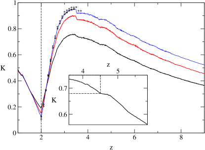
Figure 4: The generalized diffusion coefficient $K$ as a function of $z$ for the fixed height of the map $h=\sqrt{3}$ as defined in the text. Different curves correspond to simulations with $10^{6}$ trajectories and different computation times, from bottom to top on the right hand side of the figure $n=10^{2},10^{3},10^{4}$. Note the inverse order of the curves at the point $z=2$ marked by the vertical dashed line. Curves consist of $854,646,650$ points, respectively. Several values of $K$ for $n=10^{5}$ are also shown (circles). The data indicate clear convergence in time and the formation of irregularities. Additionally, several representative values of $K$ calculated for $10^{7}$ trajectories, each of the length of $10^{4}$ time steps, are shown (squares). They coincide with corresponding values of $K$ calculated with $10^{6}$ trajectories, each of the length of $10^{4}$ time steps. The inset shows a magnified region of the curve calculated for $n=10^{2}$. The dashed box marks a region that appears to be self-similar to the whole region shown in the inset indicating the existence of an underlying fractal pattern. The curve was calculated for $2\cdot 10^{7}$ trajectories and consists of $200$ points.

Now we focus on the dependence of $K$ on the parameter $h$ with the parameter of nonlinearity $z$ kept fixed. In Fig. 5 the behavior of the GDC as a function of $h$ is shown for different values of $z$ which, as expected, is more non-monotonous than that of $K(z)$. The structure of $K(h)$ for different $z$ looks somewhat similar, however, we could not detect a simple scaling. For $z=1$ the map Eq. (1) reduces to a piecewise linear map for which it was shown analytically and numerically that diffusion is normal and that the diffusion coefficient is a fractal function of the slope $a$ Kla95 ; Kla96 ; Klauss ; GrKl02 ; KlKo02 ; Kla04 , see the upper curve in Fig. 5. For $z=3$ and over a larger range of $a$, $K(a)$ as obtained from simulations is presented in Fig. 6 (a). Magnifications of the initial region, see Fig. 6 (b) and (c), show a self similar-like behavior of $K$ on finer and finer scales indicating a fractal structure.

Figure 5: The generalized diffusion coefficient $K$ as a function of parameter $h$ for different values of $z$. From top to bottom it is $z=1,2.5,3,3.5,4$. For clarity the curves are shifted vertically by $1.5,1,0.6,0.4,0.2$, respectively.

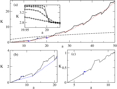
Figure 6: (a) The generalized diffusion coefficient $K$ over a large range of the parameter $a$ at $z=3$. Note that $K(3,a)=0$ for $1\leq a\leq 4$. The dashed line represents the CTRW approximation Eq. (28). The dashed-dotted line is the modified CTRW Eqs. (31), (34). (b) and (c) show magnifications of the initial region of (a) demonstrating the existence of irregularities on finer scales. The dashed line in (b) shows the modified CTRW Eqs. (32), (34). The sets of symbols included in (a) to (c) correspond to specific turnstile parameter values (see Section III for explanations). The inset in (a) depicts the development of a discontinuity in the GDC around $a=20$. The different lines correspond to different iteration times, from bottom to top at left $n=10^{3}$ (circles), $10^{4}$ (squares), $10^{5}$ (rhombuses), $10^{6}$ (triangles), thus yielding a higher numerical precision. The curve with $10^{7}$ trajectories and $10^{4}$ time steps, which coincides with the one calculated with $10^{6}$ trajectories and $10^{4}$ time steps, shows that we gain convergence with respect to the number of trajectories. The data in (a) consists of $1198$ points.

A qualitative explanation for the fractality of all these curves can be given in terms of turnstile dynamics, which has successfully been applied in order to understand the fractality of the normal diffusion coefficient in piecewise linear maps. Here we outline the basic idea of this approach only, for technical details we refer to Refs. Kla95 ; Kla96 . The key ingredient of this method is the orbit generated by iterations of the critical point $x_{c}=1/2$ of the map $M$ restricted onto the unit interval, $x_{n}=M^{n}(x_{c})\>\mbox{mod}\>1$. If this orbit is periodic it defines a Markov partition with certain partition parts representing coupling regions (turnstiles) where, in the associated periodically continued map, particles can jump from one unit interval to another one. Specific parameter values define Markov partitions with specific turnstile couplings which, in more physical terms, generate specific sequences of forward- and backward scattering of particles that start nearby the critical point. It turns out that these Markov partitions are topologically highly unstable under parameter variation, in the present case both for varying $z$ and $a$.

In Fig. 6 (a) three parameter values are identified representing Markov partitions that correspond to two local minima and a local maximum of $K(a)$ thus highlighting a specific fine structure in the whole curve. Higher-order Markov partitions can now be constructed (generated by higher-order iterations of the critical point) which are of the same type as the initial three identified in Fig. 6 (a), however, yielding new sets of parameter values. Such higher-order parameter triples are shown in Fig. 6 (b), (c). They identify the same type of fine structure on finer and finer scales. A similar analysis can be performed for other local peaks of $K(a)$ qualitatively explaining the fractal structure of the GDC. More quantitatively, one may wish to calculate some fractal dimension for these curves. However, this is a hard task even if analytical formulas for a diffusion coefficient are available Klauss and is left for further studies.

We conclude this section with an unexpected detail of the GDC. For the piecewise linear map at $z=1$ the diffusion coefficient as a function of slope of the map is continuous GrKl02 . For $z=3$, however, numerical results suggest that the dependence of $K$ on $a$ is discontinuous. In the inset of Fig. 6 we have magnified a small region of $K$ around $a=20$ (analogous behavior is found around $a=12,28,36,\ldots$). Note that for $a>20$ particles can jump for the first time from the first unit interval to the fourth one. Increasing the numerical precision by increasing the computation time, $K(a)$ near $a=20$ gradually approaches a step function, which suggests that a discontinuity develops. Similar discontinuities have already been reported for Lyapunov exponents as functions of a bias in piecewise linear maps KlCP . More complicated ones are known to exist for diffusion coefficients of nonlinear maps exhibiting bifurcation scenarios Kor02 and have recently been highlighted in research on transport in polygonal billiard channels JeRo06 . An explanation why for our model the GDC is discontinuous for $z=3$ while it is continuous for $z=1$ may be sought in the completely different character of the PDF of the map for $z=3$, which develops non-integrable singularities at all marginally stable fixed points. Details of this peculiar behavior will be discussed later, see Fig. 8 and the analysis after Eq. (52). Note that at suspected points of discontinuity of the GDC like $a=20$ the critical point is getting mapped right onto these singular regions of the PDF at the very first iteration. Simultaneously, the orbit of the critical point exhibits a transition from forward to backward scattering under variation of $a$, which leads to a local maximum of the GDC in terms of turnstile dynamics. For $z=3$ this change in the microscopic scattering process is drastically amplified by the singular behavior of the PDF probably leading to a discontinuity in the GDC. In contrast, for $z=1$ the PDF is not singular but a non-differentiable step function Kla96 , thus the GDC is locally maximal but still continuous. It would be valuable to have a mathematical proof of this conjectured discontinuity phenomenon.

The discontinuity at $a=20$ is furthermore a boundary point of the specific fine structure identified in Fig. 6, which was previously discussed in terms of turnstile dynamics. As we have just emphasized, this parameter value is determined by a specific periodic orbit of the critical point of the map. However, as was outlined before, one can now construct infinitely many higher-order iterates of the same type of periodic orbits yielding new sets of parameter values. These parameter values are related to the same type of structure and, hence, identify the same type of discontinuity on finer and finer scales. Furthermore, such parameter values are typically densely distributed on the parameter axis Kla95 ; Kla96 . This leads us to conjecture that $K(a)$ shown in Fig. 6 is discontinuous on a dense set of parameter values (probably being of measure zero). Note that the argument carries over to $K(z)$ in Fig. 4, where a careful study of the largest point of irregularity at $z\simeq 3.4$ reveals the same type of discontinuity.

So far we have focused on the fine structure of the GDC only. The next section proceeds with an understanding of its coarse functional form. As far as we know there is only one analytical result in the literature trying to predict the whole parameter dependence of the GDC of this map Gei84 . However, as we will show the respective calculation needs to be modified in order to match to computer simulation results. This necessitates to briefly review the whole approach by explaining our corrections.

IV Continuous time random walk theory for maps

The CTRW theory of Montroll, Weiss and Scher MW has become a standard tool to model diffusion in intermittent maps like Eq. (1) Gei84 ; Zum93 . This approach assumes that diffusion can be decomposed into two stochastic processes characterized by waiting times and jumps. Thus one has two sequences of independent identically distributed random variables, namely a sequence of positive random waiting times $T_{1},T_{2},T_{3},\ldots$ with PDF $w(t)$, $\int_{0}^{\infty}w(t)dt=1$, and a sequence of random jumps $\zeta_{1},\zeta_{2},\zeta_{3},\ldots$ with a PDF $\lambda(x)$, $\int_{-\infty}^{\infty}\lambda(x)dx=1$. For example, if a particle starts at point $x=0$ at time $t_{0}=0$ and makes a jump of length $\zeta_{n}$ at time $t_{n}=T_{1}+T_{2}+...+T_{n}$, its position is $x=0$ for $0\leq t<T_{1}=t_{1}$ and $x=\zeta_{1}+\zeta_{2}+...+\zeta_{n}$ for $t_{n}\leq t<t_{n+1}$. The probability that at least one jump is performed within the time interval $[0,t)$ is then $\int_{0}^{t}dt^{\prime}w(t^{\prime})$ while the probability for no jump during this time interval reads $\Psi(t)=1-\int_{0}^{t}dt^{\prime}w(t^{\prime})$. The master equation for the PDF $P(x,t)$ to find a particle at position $x$ and time $t$ is then

$$P(x,t) = \int_{-\infty}^{\infty}dx^{\prime}\lambda(x-x^{\prime})\int_{0}^{t}dt^{\prime}\;w(t-t^{\prime})\;P(x^{\prime},t^{\prime})+$$ (6)

$$+\Psi(t)\delta(x)\quad.$$

It has the following probabilistic meaning: The PDF to find a particle at position $x$ at time $t$ is equal to the PDF to find it at point $x^{\prime}$ at some previous time $t^{\prime}$ multiplied with the transition probability to get from $(x^{\prime},t^{\prime})$ to $(x,t)$ integrated over all possible values of $x^{\prime}$ and $t^{\prime}$. The second term accounts for the probability to remain at the initial position $x=0$. It is easy to check that this equation yields a normalized PDF $P(x,t)$. The most convenient representation of this equation is obtained in terms of the Fourier-Laplace transform of the PDF,

$$\hat{\tilde{P}}(k,s)=\int_{-\infty}^{\infty}dx\;e^{ikx}\int_{0}^{\infty}dt\;e^{-st}P(x,t)\quad,$$ (7)

where the hat stands for the Fourier transform and the tilde for the Laplace transform. Respectively, this function obeys the Fourier-Laplace transform of Eq. (6), which is called the Montroll-Weiss equation MW ,

$$\hat{\tilde{P}}(k,s)=\frac{1-\tilde{w}(s)}{s}\frac{1}{1-\hat{\lambda}(k)\tilde{w}(s)}\quad.$$ (8)

The Laplace transform of the MSD can be readily obtained by differentiating the Fourier-Laplace transform of the PDF,

$$\tilde{\left<x^{2}(s)\right>}=\int_{-\infty}^{\infty}dx\;x^{2}\tilde{P}(x,s)=\left.-\frac{\partial^{2}\hat{\tilde{P}}(k,s)}{\partial k^{2}}\right|_{k=0}\quad.$$ (9)

In order to calculate the MSD within this theory, it thus suffices to know $\lambda(x)$ and $w(t)$ generating the stochastic process. For one-dimensional maps of the type of Eq. (1), using the symmetry of the map the waiting time distribution can be calculated from the approximation

$$x_{n+1}-x_{n}\simeq\frac{dx_{t}}{dt}=ax_{t}^{z},\;\;x_{t}\ll 1\quad,$$ (10)

where we have introduced the continuous time $t\geq 0$. Solving this equation for initial condition $x_{0}$ yields

$$x_{t}=\left[\frac{1}{x_{0}^{z-1}}-a(z-1)t\right]^{-\frac{1}{z-1}}\quad.$$ (11)

We now define that a particle makes a jump when it leaves the unit interval. Note that this definition is different from the one of Ref. Gei84 , which used the interval $[-\frac{1}{2},\frac{1}{2}]$. That the unit interval is the right choice for calculating the parameter-dependent random walk diffusion coefficient was shown for $z=1$ in Refs. Kla95 ; Kla96 ; KlDo97 ; KlKo02 ; Kla02 . From Eq. (11) one can then obtain the time $t$ that a particle spends on the unit interval before making a jump according to the condition $x_{t}=1$. The waiting time thus becomes a function of the injection point $x_{0}$,

$$t(x_{0})=\frac{1}{a(z-1)}\left(\frac{1}{x_{0}^{z-1}}-1\right)\quad.$$ (12)

Accordingly, the waiting time PDF $w(t)$ is related to the yet unknown PDF of injection points,

$$w(t)\simeq P_{in}(x_{0})\left|\frac{dx_{0}}{dt}\right|\quad.$$ (13)

Making the assumption that the PDF of injection points is uniform, $P_{in}\simeq 1$, the waiting time PDF is calculated to

$$w(t)=a\left[1+a(z-1)t\right]^{-\frac{z}{z-1}}$$ (14)

for long enough times $t$, where normalization is used to obtain the prefactor.

If jumps between neighboring cells only are taken into account, the jump PDF and its Fourier transform may be assumed as Zum93

$$\lambda(x)=\delta(|x|-1),\;\;\;\hat{\lambda}(k)=\cos(k)\quad.$$ (15)

Combining Eq. (9) with Eq. (15) leads to the Laplace transform Gei84

$$\tilde{\left<x^{2}\right>}=\frac{\tilde{w}(s)}{s(1-\tilde{w}(s))}\quad.$$ (16)

For the following calculations it is useful to define

$$\gamma:=\frac{1}{z-1}\>,\>z>1\quad.$$ (17)

Note that for $z\geq 2$, $\gamma$ is identical with $\beta$ defined in Eq. (4). For $\gamma\neq 2$ the Laplace transform of Eq. (14) reads

$$\tilde{w}(s)=\gamma(bs)^{\gamma}e^{bs}\Gamma(-\gamma,bs)=1-(bs)^{\gamma}e^{bs}\Gamma(1-\gamma,bs)\>,$$ (18)

with $b:=\gamma/a$ and the incomplete Gamma function $\Gamma(a,x):=\int_{x}^{\infty}dt\;e^{-t}t^{a-1}$.

For $\gamma=1$ the Laplace transform of the waiting time distribution is

$$\tilde{w}(s)=1-\frac{2s}{a}e^{\frac{2s}{a}}E_{1}(\frac{2s}{a})\quad,$$ (19)

where $E_{1}(x)$ is the exponential integral, $E_{1}(x):=-ei(-x)=\int_{x}^{\infty}dt\frac{e^{-t}}{t}$.

Here we are only interested in the long time behavior of the MSD, which corresponds to taking the limit $s\rightarrow 0$ in Eqs. (18), (19) with $\gamma$ being constant. For $0<\gamma<1$, taking the lowest order of the expansion we get $\Gamma(1-\gamma,bs)\simeq\Gamma(1-\gamma)$ and

$$\tilde{w}(s)\simeq 1-(bs)^{\gamma}\Gamma(1-\gamma)\quad.$$ (20)

Eq. (16) then yields

$$\tilde{\left<x^{2}\right>}=\frac{1}{\Gamma(1-\gamma)b^{\gamma}}s^{-1-\gamma}$$ (21)

and its inverse Laplace transform is

$$\left<x^{2}\right>=\frac{a^{\gamma}\sin(\pi\gamma)}{2\pi\gamma^{1+\gamma}}t^{\gamma},\;\;\;0<\gamma<1\quad.$$ (22)

Similarly, for the normal diffusive case $\gamma>1$ we get from Eq. (18) as the small $s$-asymptotics of the waiting time distribution

$$\tilde{w}(s)\simeq 1-\frac{bs}{\gamma-1}$$ (23)

Using Eq. (16) and the inverse Laplace transform yields

$$\left<x^{2}\right>=\frac{\gamma-1}{b}\;t,\;\;\;\gamma>1\quad.$$ (24)

In the remaining case $\gamma=1$, the expansion of the exponential integral is $ei(-x)=\ln(x)+\tilde{\gamma}$, where $\tilde{\gamma}$ is Euler’s constant. For small $s$ Eq. (19) reads

$$\tilde{w}(s)\simeq 1+bs\ln(bs)$$ (25)

and Eq. (16) gives

$$\tilde{\left<x^{2}\right>}=\frac{b^{-1}s^{-2}}{\ln(1/bs)}-\frac{1}{s}\quad.$$ (26)

The inverse Laplace transform of the first term can be obtained by applying Karamata’s Tauberian theorem Bingham , which relates the Laplace transform of a function given in the form $f(s)\sim A\frac{\Gamma(1+\gamma)}{s^{\gamma+1}}L(1/s)$ for $s\rightarrow 0$ and $\gamma>-1$ to the inverse $F(t)\sim At^{\gamma}L(t)$ for $t\rightarrow\infty$. The function $L$ must meet the requirement of being slowly varying, $\frac{L(ux)}{L(x)}\rightarrow 1$ for $u>0$ as $x\rightarrow\infty$. In our case we have $\gamma=1$, $\Gamma(2)=1$ and the function $L(1/s)=\frac{1}{\ln(1/bs)}$ satisfies the above condition. For the MSD we thus get

$$<x^{2}>=\frac{at}{\ln(at)}\quad,\quad\gamma=1\quad.$$ (27)

In summary, we obtain for the GDC

$$K=\begin{cases}\frac{a^{\gamma}\sin(\pi\gamma)}{\pi\gamma^{1+\gamma}}\quad,&0<\gamma<1\cr 0\quad,&\gamma=1\cr a\frac{\gamma-1}{\gamma}\quad,&\gamma>1\end{cases}$$ (28)

with $\gamma=\frac{1}{z-1}$. For $\gamma=1$ we get $K=0$ because of the logarithmic term in Eq. (27).

Now we compare this result with our numerical simulations. As an example, $K$ as a function of $a$ determined by Eq. (28) is shown in Fig. 6 (a), where $z=3$. For $z>2$, the difference to the result of Ref. Gei84 is by a factor of two. This yields approximately the right slope for small $a$, however, it does not reproduce the trivial value of $K(4)=0$ when particles cannot escape from the unit interval anymore. Hence, further modifications are necessary.

V Modified CTRW theory

The easiest way to modify standard CTRW theory is by varying either the waiting time or the jump PDF. However, the waiting time distribution is straightforwardly determined by the model as a power law for all intermittent values of $z$. This suggests to change the jump PDF Eq. (15) only, which in a first attempt one may write as

$$\lambda(x)=\frac{p}{2}\delta(\left|x\right|-1)+(1-p)\delta(x)\quad.$$ (29)

Here the second term reflects the fact that the particle can stay on the unit interval with probability $(1-p)$. By assuming that the density of particles is uniform on the unit interval, $p$ is determined by the size of the escape region, $p(a)=2\Delta(a)$ with $\Delta=\frac{1}{2}-x_{c}$, where $x_{c}$ is the solution of the equation $x_{c}+ax^{z}_{c}=1$. For normal diffusion it is well-known that $K_{rw}=p(a)$ provides a random walk approximation for the diffusion coefficient which is asymptotically correct in case of nearest neighbor jumps, $p(a)\ll 1$ Kla95 ; Kla96 ; KlDo97 ; KlKo02 . For farther than nearest neighbor jumps this approximation is straightforwardly generalized by weighting the integer jump distance squared with the respective probability, based on the escape region, to perform such a jump Kla02 . Assuming that one knows about the power law time dependence of the MSD Eq. (2) for this map, one can apply the same approximation to anomalous diffusion. In Fig. 7 the result is shown for $K(z)$ at $a=5$. As one can see, this simple argument indeed roughly reproduces the coarse functional form of $K(z)$ and yields the exact value at $z=1$.

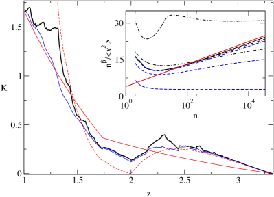
Figure 7: $K$ as a function of $z$ for $a=5$. The bold black line depicts again the computer simulation results from Fig. 3. The thin line that is on top at $z=2$ represents the simple random walk approximation Eq. (36) for $i=2$. The dashed line corresponds to the modified CTRW approximation Eqs. (32), (34). The thin line that is in the middle at $z=2$ displays the first term of the TGK formula Eq. (53). The inset reveals the existence of logarithmic corrections in the MSD by plotting $n^{\beta}/\left<x^{2}\right>$ with respect to $\ln n$ for $a=3.14$ and different $z$ close to the transition point at $z=2$. The dashed lines correspond to $z=1.5,1.9,1.95$ from bottom to top, the dashed-dotted lines to $z=2.5,2.1,2.05$ from top to bottom. The thick solid line represents $z=2$, the thin solid line is proportional to $\ln n$ as a guide for the eye.

Accordingly, the modification of standard CTRW theory Eq. (29) works for nearest neighbor jumps only. We thus further amend the jump pdf Eq. (29) by introducing a typical jump length $l$,

$$\lambda(x)=\frac{p}{2}\delta(\left|x\right|-l)+(1-p)\delta(x)\quad,$$ (30)

with Fourier transform $\hat{\lambda}(k)=p\cos(lk)+1-p$. This jump length we define either by the actual mean displacement

$$l_{1}=\left\{|M(x)-x|\right\}$$ (31)

or, under the simplifying assumption of integer jumps, by the coarse-grained displacement

$$l_{2}=\left\{|[M(x)]|\right\}\quad,$$ (32)

where the square brackets hold for the largest integer less than the argument. Here the averages, denoted by curly brackets, are performed starting from a uniform initial ensemble of walkers with respect to the conditional probability density that particles leave the unit interval. The latter ensemble averages are then averaged over time. Repeating the calculations from the previous section with Eq. (30), we obtain the MSD

$$\left<x^{2}\right>=pl_{i}^{2}\begin{cases}\frac{a^{\gamma}\sin(\pi\gamma)}{\pi\gamma^{1+\gamma}}\;t^{\gamma}\quad,&0<\gamma<1\cr\frac{at}{\ln(at)}\quad,&\gamma=1\cr\frac{\gamma-1}{\gamma}\;at\quad,&\gamma>1\quad,\end{cases}$$ (33)

$i=1,2$, where the typical jump length $l_{i}$ is given by Eqs. (31), (32). Hence, our final CTRW expression for the GDC reads fnote3

$$K=pl_{i}^{2}\begin{cases}\frac{a^{\gamma}\sin(\pi\gamma)}{\pi\gamma^{1+\gamma}}\quad,&0<\gamma<1\cr 0\quad,&\gamma=1\cr a\frac{\gamma-1}{\gamma}\quad,&\gamma>1\quad.\end{cases}$$ (34)

Fig. 6 (a) shows the CTRW approximation Eq. (34) with jump length $l_{1}$, Eq. (31), which describes the coarse dependence of the GDC very well over a large range of parameters. The CTRW result with integer jump length $l_{2}$, Eq. (32) with Eq. (34), is shown in Fig. 6 (b). It gives an asymptotically exact approximation of the GDC for small values of $a$, however, it also holds well for larger parameters. A quantitative comparison moreover indicates (within numerical accuracy) that this combination yields results which exactly correspond to our numerical findings for $K$ at all integer values of $h=M(\frac{1}{2})>0$, which for $z=3$ are equivalent to $a=4,12,20,...$. This generalizes results obtained previously for the normal diffusion coefficient at $z=1$ Kla96 ; KlDo97 .

We now focus on $K$ as a function of $z$. Fig. 7 shows the modified CTRW approximation Eqs. (32), (34) in comparison with simulation results. In the strongly anomalous regime of large $z$ the approximation reproduces the GDC from simulations very well, however, for smaller values of $z$ there are obvious deviations. Let us first explain the problem for $z\to 1$, the region around $z=2$ will be discussed in the following section.

Let us recall that according to Eqs. (2),(4), for $z<2$ the map exhibits normal diffusion in the long-time limit. One can further split this regime into $3/2\leq z<2$, where the MSD shows transient anomalous diffusion which becomes normal for long times while for $1\leq z<3/2$ it represents purely normal dynamics Gas88 . However, in the latter case it is well-known that the waiting time distribution is exponential Kla96 ,

$$w(t)=\tilde{\gamma}e^{-\tilde{\gamma}t}\quad,$$ (35)

where $\tilde{\gamma}$ is the escape rate, and not a power law such as the CTRW approximation Eq. (14). In fact, in the limit of $z\to 1$ Eq. (34) leads to $K=apl_{i}^{2}$, whereas the correct random walk result for normal diffusion reads Kla96 ; KlDo97

$$K=pl_{i}^{2}\quad.$$ (36)

Note that for $z\to 1$ and by assuming a uniform density on the unit interval, in case of $l_{2}\ll 2$ this equation yields $K=p$, whereas for $l_{2}\gg 2$ we get $K=l_{2}^{2}$ thus recovering the two simple random walk results mentioned earlier. Eq. (36) is indeed straightforwardly obtained from CTRW theory if one repeats the calculations with the exponential waiting time distribution Eq. (35) and $\tilde{\gamma}=1$, i.e., by assuming that on average a particle leaves the unit cell after one time-discrete jump. We thus conclude that the CTRW result Eq. (34) gives only a reliable approximation for the GDC if $\gamma\leq 2$, whereas for $\gamma>2$ the simple random walk result for normal diffusion Eq. (36) should be used. This is in line with Fig. 7.

VI Suppression of the GDC at a dynamical transition

Let us now understand the behavior of $K(z)$ around $z=2$, where the map exhibits a dynamical transition Beck ; Wang from normal to anomalous diffusion, see Eqs. (2),(4). Interestingly, this transition is clearly visible in the strength of the GDC, which to our knowledge has not been reported before. We now explain this phenomenon in detail.

As mentioned in Section III, around the transition point there are significant deviations between CTRW theory and the simulation results. These differences are displayed in Fig. 7. At $z=2$ the CTRW approximation forms a non-differentiable little wedge with $K(2)=0$ at the minimum, whereas the simulations yield $K(2)>0$. We recall that by increasing the computation time there is some slow convergence of the simulation data towards the CTRW solution, see the inset of Fig. 3, but that we were not able to achieve quantitative agreement with the CTRW prediction of $K(2)=0$.

This very slow convergence of the simulation results as well as the logarithmic term in the MSD at $z=2$, see Eq. (33), suggest that the deviations between simulations and CTRW theory are due to logarithmic corrections in the MSD for parameter values around $z=2$. Curiously, such terms are not present in Eq. (33) for $z\neq 2$ ($\gamma\neq 1$). By refining our CTRW analysis, we will now show that such logarithmic terms indeed exist. However, for $z\neq 2$ they hold for large but finite times only, whereas for $z=2$ they persist in the limit of infinite time. As is obvious from Eqs. (33), (34), for $z=2$ the surviving logarithmic term leads to a full suppression of the GDC, whereas close to the transition point finite-time logarithmic corrections yield a gradual suppression of the strength of diffusion.

We start again from the exact expression for the Laplace transform of the waiting time PDF $\tilde{w}(s)$, Eq. (18). Combining this equation with the jump PDF Eq. (30) and Eqs. (8), (9) we obtain the Laplace transform of the MSD

$$\tilde{\left<x^{2}\right>}=pl_{i}^{2}b^{-\gamma}s^{-1-\gamma}e^{bs}\Gamma^{-1}(1-\gamma,bs)-\frac{pl_{i}^{2}}{s}\quad.$$ (37)

We immediately drop the second term, since its inverse Laplace transform is simply constant. Let us focus now on the limits $s\to 0$ and $\gamma\to 1$. In case of $0<\gamma\leq 1$ the $\Gamma$ function in Eq. (37) can be expanded to

$$\Gamma(1-\gamma,bs)=\Gamma(1-\gamma)-\frac{(bs)^{1-\gamma}}{1-\gamma}-\sum_{j=1}^{\infty}\frac{(-1)^{j}(bs)^{j+1-\gamma}}{(j+1-\gamma)j!}\quad.$$ (38)

From this equation it follows that as $\gamma$ approaches $1$ from below one may consider not only the first term as in Eq. (20) but also the second one, since both terms are divergent for $\gamma\to 1^{-}$. All other terms are nonsingular and can be safely neglected. We further expand the second term of Eq. (38) to

$$\frac{(bs)^{1-\gamma}}{1-\gamma} = \frac{e^{(1-\gamma)\ln(bs)}}{1-\gamma}$$

$$= \frac{1}{1-\gamma}+\ln(bs)+\sum_{j=2}^{\infty}\frac{(1-\gamma)^{j-1}}{j!}\;(\ln(bs))^{j}\quad.$$

Note that here we have obtained a series of logarithmic terms which, as we shall see, provides the logarithmic corrections we are looking for. By imposing the condition that $|(1-\gamma)\ln(bs)|<1$, we may keep only the first two terms of Eq. (LABEL:s2),

$$\frac{(bs)^{1-\gamma}}{1-\gamma}\simeq\frac{1}{1-\gamma}+\ln(bs)\quad.$$ (40)

Finally, we expand the first term of Eq. (38) to

$$\Gamma(1-\gamma)=\frac{1}{1-\gamma}-\tilde{\gamma}+\sum_{j=2}^{\infty}\frac{(1-\gamma)^{j}}{j!}\int_{0}^{\infty}dt\;e^{-t}(\ln t)^{j}\quad,$$ (41)

where $\tilde{\gamma}$ is again Euler’s constant. Because we are interested in the small $\gamma$ limit, we keep only the first term of this expansion. In summary, we obtain for the Laplace transform of the MSD Eq. (37) in the limits of $|(1-\gamma)\ln(bs)|<1$ and $\gamma\to 1^{-}$

$$\tilde{\left<x^{2}\right>}=pl_{i}^{2}b^{-\gamma}s^{-1-\gamma}\;\frac{1}{\ln(\frac{1}{bs})}\quad.$$ (42)

Inversion of the Laplace transform yields as the final result

$$\left<x^{2}\right>=\frac{pl_{i}^{2}t^{\gamma}}{b^{\gamma}\Gamma(1+\gamma)\ln(t/b)},\quad t<t_{cr}$$ (43)

with $t_{cr}:=be^{1/(1-\gamma)}$. For $t\gg t_{cr}$ and $0<\gamma<1$ one can drop the second term in the $\Gamma$ function expansion Eq. (38), and the asymptotic CTRW result Eq. (33) is recovered. Interestingly, $t_{cr}$ diverges when $\gamma\to 1^{-}$, and at $\gamma=1$ one thus arrives at the asymptotic $t/\ln t$ dependence of Eq. (33).

Analogous corrections are obtained for $1<\gamma$ near the dynamical transition point, $\gamma\to 1^{+}$. By applying the same arguments as above we get

$$\left<x^{2}\right>=\frac{pl_{i}^{2}t}{b^{\gamma}\Gamma(1+\gamma)\ln(t/b)},\quad t<\tilde{t}_{cr}\quad,$$ (44)

where $\tilde{t}_{cr}:=be^{1/(\gamma-1)}$. In the long time limit we again recover the CTRW asymptotics Eq. (33) fnote .

These analytical findings are in agreement with results from computer simulations. In the inset of Fig. 7, $n^{\beta}/\left<x^{2}\right>$ is shown as a function of $\ln n$ close to the transition point at $z=2$ for different values of $z$ and $a=3.14$. The logarithmic corrections are less obvious if $z$ is sufficiently different from $2$, where $n^{\beta}/\left<x^{2}\right>$ quickly converges to $1/K$. However, the logarithmic corrections are getting significant when $z$ approaches the dynamical transition value. We have thus identified the precise dynamical origin of the suppression of the GDC at $z=2$.

Dynamical transitions are quite ubiquitous in intermittent maps and have been widely discussed in the literature in terms of the time dependence of the MSD. However, it appears that so far no attention has been paid to a possible critical behavior of the associated GDC. Our results lead us to conjecture that suppression and enhancement of the GDC are typical for dynamical transitions in anomalous dynamics altogether Zum93a .

VII Time-fractional equation for subdiffusion

The great success of the CTRW approach is related to the fact that it not only predicts the power $\gamma$ but also the form of the coarse grained PDF $P(x,t)$ of displacements Zum93 . Correspondingly the anomalous diffusion process generated by our model is not described by an ordinary diffusion equation but by a fractional generalization of it. Starting from the Montroll-Weiss equation and making use of the expressions for the jump and waiting time PDFs Eqs. (14), (15), we rewrite Eq. (8) in the long-time and -space asymptotic form

$$s^{\gamma}\hat{\tilde{P}}-s^{\gamma-1}=-\frac{pl_{i}^{2}}{2cb^{\gamma}}k^{2}\hat{\tilde{P}}$$ (45)

with $c=\Gamma(1-\gamma)$ and $b=\gamma/a$. For the initial condition $P(x,0)=\delta(x)$ of the PDF we have $\hat{P}(k,0)=1$. It is now helpful to recall the definition of the Caputo fractional derivative of a function $G$

$$\frac{\partial^{\gamma}G}{\partial t^{\gamma}}:=\frac{1}{\Gamma(1-\gamma)}\;\int_{0}^{t}dt^{{}^{\prime}}(t-t^{{}^{\prime}})^{-\gamma}\frac{\partial G}{\partial t^{{}^{\prime}}}$$ (46)

and its Laplace transform Podl ; Mai97 ,

$$\int_{0}^{\infty}dt\;e^{-st}\frac{\partial^{\gamma}G}{\partial t^{\gamma}}=s^{\gamma}\tilde{G}(s)-s^{\gamma-1}G(0)\quad.$$ (47)

Noticing that the left part of Eq. (45) precisely coincides with the Laplace transform of the Caputo derivative of the PDF and turning back to real space, we arrive at the time-fractional diffusion equation

$$\frac{\partial^{\gamma}P(x,t)}{\partial t^{\gamma}}=D\;\frac{\partial^{2}P}{\partial x^{2}}$$ (48)

with $D$ given by the modified CTRW theory Eqs. (3), (34). Time-fractional diffusion equations of such a form have already been extensively studied by mathematicians Gor00 . Note that in application to our model another version of such an equation was proposed in Ref. Bar03 , which uses a Riemann-Liouville fractional derivative. It can be easily shown that both forms of time-fractional diffusion equations are equivalent under rather weak assumptions ACunp . Yet two other forms of subdiffusive fractional equations (however, not with applications to maps) were proposed in Refs. Sai97 and Met00 . Again, after some recasting these equations yield Eq. (48) LUnp .

The solution of Eq. (48) is expressed in terms of an M-function of Wright type Mai97 ,

$$P(x,t)=\frac{1}{2\sqrt{D}t^{\gamma/2}}M\left(\xi,\frac{\gamma}{2}\right)$$ (49)

with $\xi:=|x|/\sqrt{D}t^{\gamma/2}$, where we use the representation of the M-function

$$M(z,\gamma)=\frac{1}{\pi}\sum_{i=1}^{\infty}\frac{(-z)^{i-1}}{(i-1)!}\Gamma(\gamma i)\sin(\gamma i\pi)\quad.$$ (50)

This solution gives exactly the same asymptotics that was obtained in Ref. Zum93 for small and large values of $\xi$,

$$P(x,t)\simeq t^{-\gamma/2}\begin{cases}1-a_{1}\xi+a_{2}\xi^{2}\quad,&\xi\ll 1\cr\xi^{\frac{\gamma-1}{2-\gamma}}\exp(-b_{1}\xi^{\frac{2}{2-\gamma}})\quad,&\xi\gg 1\quad,\end{cases}$$ (51)

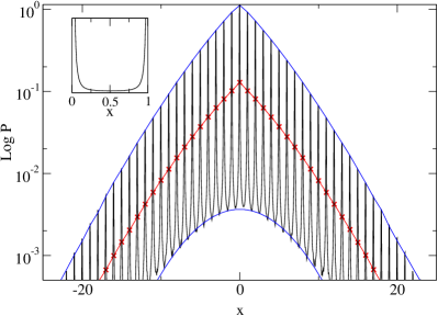
Figure 8: Main figure: The oscillatory structure shows the PDF obtained from simulations of the map Eq. (1) for $z=3$ and $a=8$. The simulated PDF was computed from an ensemble of $10^{7}$ trajectories after $n=10^{3}$ iterations. The crosses (x) represent the simulated PDF coarse-grained over unit intervals. The continuous line in the middle yields the analytical solution of the fractional diffusion equation Eq. (49) with the same $z$ while $D$ is taken from simulations. The upper and the lower curves correspond to fits with an M-function form, calculated with the same $z$ but for different $D$, and a Gaussian form, respectively. More explanations are provided in the text, see Sec.VII below. The inset depicts schematically the simulated PDF for the map Eq. (1) modulo $1$.

where $a_{1},a_{2},b_{1}$ are some constants that are given explicitly in Ref. Zum93 .

Similar to the modified CTRW approximation of the parameter-dependent GDC we now find that the analytical PDF Eq. (49) describes only the coarse scale of the PDF obtained from simulations but not its fine structure. This mismatch can be understood related to the fact that our model consists of a periodic lattice defined by specific elementary cells. Any elementary cell develops a characteristic “microscopic” PDF, characterized by the map Eq. (1) restricted onto the unit interval, which exhibits singularities at the marginally stable fixed points. The inset of Fig. 8 schematically depicts such a PDF of an elementary cell after a large number of iterations. Precisely this functional form yields the building block for the PDF of the periodically continued map, see the main part of Fig. 8. If one eliminates the fine structure by averaging over whole unit intervals, one obtains a coarse-grained PDF that is in excellent agreement with the analytical solution of the fractional diffusion equation Eq. (48), see Fig. 8.

Such an interplay between the “microscopic” PDF of a single scatterer and the “macroscopic” PDF of the spatially extended system was already reported for the normal diffusive model at $z=1$ Kla96 ; Kla02 ; Kla04 and was recently also studied in billiards Sand05 . However, in case of anomalous diffusion the PDF exhibits a further remarkable property: Fig. 8 shows that the oscillatory structure of the whole PDF is bounded by two different functions. The upper curve is of M-function type and connects all local maxima of the microscopic PDF. These maxima are situated in regions of the map where the dynamics is regular, due to the marginally stable fixed points. The lower curve, on the other hand, is Gaussian and is determined by all local minima of the microscopic PDF. These minima are generated in regions of the map being far away from the marginally stable fixed points, where the dynamics is locally most strongly chaotic fnote2 . Fig. 8 thus nicely exemplifies the microscopic origin of anomalous diffusion in terms of intermittency.

VIII Taylor-Green-Kubo approach and fractal functions

We now turn back to the parameter dependence of the GDC. In Section V we have shown that an amended CTRW theory correctly describes the coarse dependence of the model’s GDC, whereas the fractal fine structure is not captured by this approach. This reflects the fact that CTRW theory is a purely stochastic approach involving a randomness assumption between jumps, see the approximations involved as outlined in Section IV and V, whereas the origin of the fractality of the GDC lies in the existence of long-range deterministic dynamical correlations, see the analysis in Section III.

This motivates us to propose an alternative approach for analyzing the GDC, which is based on the Taylor-Green-Kubo (TGK) formula Tay21 ; Kubo for diffusion in maps. This theory has successfully been applied to the fractal diffusion coefficient of the normal diffusive map at $z=1$, where it could partly be worked out analytically Kla96 , to a nonlinear map with a complicated bifurcation scenario Kor02 and to normal diffusion in billiards KlKo02 . An advantage of this analysis is that it systematically incorporates dynamical correlations. A disadvantage is that, in contrast to CTRW theory, for the map under consideration we could implement it only numerically.

The basic idea is to generalize the TGK formula for maps to anomalous diffusion. Following the usual derivation Tay21 ; KlKo02 , the first step is to transform the MSD in Eq. (2) into sums over increments, or velocities, $v_{k}:=x_{k+1}-x_{k}$,

$$<(x_{n}-x_{0})^{2}>=<\sum_{k=0}^{n-1}v_{k}\sum_{l=0}^{n-1}v_{l}>\>(n\to\infty)\>.$$ (52)

For normal diffusion the second step requires to define the ensemble average expressed by the angular brackets in terms of the invariant PDF obtained for the map restricted onto the unit interval. In case of the map Eq. (1) this still works for $z<2$, where the dynamics of the spatially extended map is normal diffusive. However, for $z\geq 2$ it is well-known that the map of the elementary cell does not possess a non-trivial invariant PDF anymore. Mathematical analysis Hu95 shows that in this case there exist two physically relevant invariant measures, one which is concentrated on the marginally stable fixed points and one that lies in-between on the interval $(0,1)$. The first measure has still nice, so-called SRB properties and yields a PDF in form of a $\delta$-distribution on the marginally stable fixed points. The second one, however, is not normalizable anymore and hence is called an infinite invariant measure. In other words, if one starts a computer simulation from an ensemble of points uniformly distributed on the unit interval, the underlying stochastic process is not stationary and the PDF of an elementary cell, computed by a histogram method, does not converge in time to a well-defined invariant PDF Zum93a ; Gas88 .

Consequently, in contrast to normal diffusion Eq. (52) cannot further be simplified by using time-translational invariance, and for the GDC Eq. (3) we have to stop at

$$K=\lim_{n\rightarrow\infty}\frac{1}{n^{\beta}}\left[<\sum_{k=0}^{n-1}v_{k}^{2}>+2<\sum_{k=0}^{n-1}\sum_{l=1}^{n-1}v_{k}v_{k+l}>\right]\>.$$ (53)

In numerical simulations we find that the first term alone is already proportional to $n^{\beta}$. If the system is ergodic, as for $z<2$ in our model, this term boils down to $n<v_{0}^{2}>$, and by neglecting any higher-order terms in Eq. (53) we recover the random walk result for normal diffusion Kla96 ; KlKo02 ; KlDo97 . For $z\geq 2$ the situation is again more complicated. Here only generalized ergodic theorems may hold Lutz04 ; Hu95 , which is intimately related to the existence of infinite invariant measures as outlined above. Whether in this case a CTRW result such as Eq. (34) can be extracted from the first term is a non-trivial open question.

However, considering the first term only as an approximation of $K$ for all $z$, the numerical results are depicted in Fig. 9. The comparison of this approximation with the previous simulation results shows that this term provides a first little step beyond a modified CTRW approach, since it reproduces the major irregularities of $K$ as a function of $a$ and even follows the suspected discontinuities discussed in Section III. However, our numerical precision is not sufficient to conclude whether it yields exact values for $K$ at integer heights.

Eq. (53) thus provides a suitable starting point for a systematic evaluation of the fractal structure of the GDC. Since the series expansion in Eq. (53) is exact, working out further terms one should recover more and more structure in the GDC on fine scales KlKo02 ; Kor02 . Interestingly, the second term in Eq. (53) can be understood as a velocity autocorrelation function that, in contrast normal diffusion, depends on two time scales. The existence of a second time scale points to the phenomenon of aging in dynamical systems Bar03 ; Rad04 . In our case this can be understood as a consequence of infinite invariant measures.

Here we do not further pursue these questions but focus instead onto a direct link between the GDC and fractal functions as provided by the TGK formula, see Refs. Kla96 ; KlKo02 ; Kor02 for normal diffusion. As was shown in Ref. KlKo02 , Eq. (53) also holds if the velocities $v_{k}$ are replaced by the integer velocities $j_{k}:=[x_{k+1}]-[x_{k}]$. It is now useful to start from $K$ expressed again by Eq. (52), trivially rewritten as

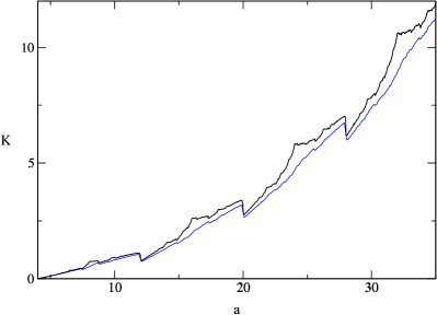
Figure 9: Comparison of the first term of the anomalous TGK formula Eq. (53) (lower line) with the computer simulation results from Fig. 6 (a).

$$K=\lim_{n\to\infty}\frac{1}{n^{\beta}}<\sum_{k=0}^{n-1}j_{k}\sum_{l=0}^{n-1}j_{l}>\quad.$$ (54)

The two sums suggest to define the jump function

$$J_{n}(x):=\sum_{k=0}^{n}j_{k}\quad,$$ (55)

which satisfies the recursion relation Kla96

$$J_{n}(x)=j_{0}(x)+J_{n-1}(M(x))\quad.$$ (56)

The jump function gives the integer value of the displacement of a particle after $n$ time steps, which started at some initial position $x\equiv x_{0}$. It thus contains essential information about the microscopic scattering process of a particle by showing how sensitively the displacement depends on initial conditions. Eqs. (54), (55) imply

$$K=\lim_{n\to\infty}\frac{1}{n^{\beta}}<J_{n-1}^{2}(x)>\quad.$$ (57)

Fig. 10 displays the product of jump functions $J_{n}^{2}(x)$, which governs the anomalous diffusion process, for a representative parameter value. Clearly, as time evolves the structure of this function is getting more complicated. The GDC, in turn, is determined by the cumulative function

$$T_{n}^{2}(x):=\int_{0}^{x}dy\;J^{2}_{n}(y)\quad,$$ (58)

where we fix the integration constants by the condition that $T_{n}^{2}(0)=0$ and by requiring that the whole function is continuous. Integration of Eq. (56) would yield a recursive functional equation for $T_{n}^{2}(x)$, which is of the same type as the one derived in Ref. Kor02 . The solutions of such equations are generalized de Rham-, respectively generalized Takagi functions Kla96 ; Kor02 . However, at present such generalized de Rham-equations cannot be solved analytically, hence we do not work out the details but instead compute $T_{n}^{2}(x)$ directly from simulations, according to the definition Eqs. (55), (58). Results for the first four iterations of $T_{n}^{2}(x)$ are shown in Fig. 11. With respect to the construction of $T_{n}^{2}(x)$, it may not come too much as a surprise that in the limit of $n\to\infty$ this function exhibits a fractal structure. Interestingly, the GDC is obtained by integrating over this structure. If one starts from a uniform ensemble of initial conditions the result reads

Figure 10: The first four iterations of the jump function $J^{2}_{n}(x)$ defined by Eq. (55) for $z=3$, $a=8$, $n=0,1,2,3$ based on a uniform ensemble of $N=10^{3}$ initial conditions. Note that there emerges a complicated fine structure.

$$K=\lim_{n\to\infty}\frac{1}{n^{\beta}}T_{n}^{2}(1)\quad.$$ (59)

This equation relates the GDC to a fractal function representing the microscopic scattering process of our model. The numerical result for the GDC Eq. (59) is in good agreement with the one employing the MSD. In the light of Fig. 11 and Eq. (59), it may not be too surprising anymore that under parameter variation a highly non-trivial GDC is obtained from this model.

Figure 11: The first four iterations of the generalized de Rham-type function $T_{n}^{2}(x)$ as defined by Eq. (58), which is obtained by numerically integrating $J_{n}^{2}(x)$ depicted in Fig. 10. The parameter values are the same as in Fig. 10. Note that there emerges a fractal structure.

IX Conclusions

In this paper we have studied subdiffusion generated by a paradigmatic one-dimensional intermittent map. In contrast to previous works here we focused onto the parameter dependence of the GDC, which is an anomalously diffusive generalization of the diffusion coefficient known for normal diffusion. Computer simulations suggested that this GDC is a fractal function of control parameters. This finding was corroborated by a qualitative explanation of the fractal structure in terms of complicated sequences of forward- and backward scattering (turnstile dynamics), which are topologically unstable under parameter variation. Our analysis furthermore led us to conjecture that the GDC is a discontinuous function of control parameters.

In trying to understand the coarse functional form of the GDC, we applied standard CTRW theory to our model. By suitably amending previous calculations, we arrived at analytical approximations that enabled us to reproduce the whole coarse functional form of the GDC yielding asymptotically exact results in the limit of large and small parameter values. However, there are clear deviations between this theory and simulations around a dynamical transition from normal to anomalous diffusion. By refining our amended theory, we were able to explain these deviations in terms of logarithmic corrections leading to ultra-slow convergence of our simulation results and eventually yielding a full suppression of the GDC right at the transition point. These findings were confirmed by simulations of the MSD.

We then studied in detail the PDF of our model. We first derived a time-fractional subdiffusion equation from CTRW theory. The coarse-grained PDF of our model turned out to be in excellent agreement with the non-Gaussian solution of our fractional diffusion equation. On a fine scale, however, the simulation results yielded an oscillatory structure reflecting the microscopic details of the intermittent scattering process. This structure was generated by the invariant density of the single scatterers hence revealing an interesting interplay between microscopic scattering and macroscopic diffusion.

A more detailed understanding of the GDC was finally provided in terms of an anomalous TGK formula, which again is a generalization of the TGK formula for normal diffusion. The structure of this formula points at intimate relations to infinite invariant measures, aging, and generalized de Rham-type fractal functions. All these terms define very active topics of research. We thus hope that, along these lines, in future work more detailed relations between mathematical infinite ergodic theory and the physics of anomalous diffusive processes can be established.

In the present paper we have only studied a one-dimensional subdiffusive map, however, we expect these findings to be typical for spatially extended, low-dimensional, anomalous deterministic dynamical systems altogether. Further studies may also focus on the relation between the anomalous TGK formula and CTRW theory, on a spectral analysis of the Frobenius-Perron operator of this model, and on analyzing a superdiffusive map by similar methods.

The authors gratefully acknowledge helpful discussions with J. Dräger, R. Gorenflo, J. Klafter, R. Metzler and A. Pikovsky. They thank the MPIPKS Dresden for hospitality and financial support. AVC acknowledges financial support from the DFG.

References

- (1) J.-P. Bouchaud, A. Georges, Phys. Rep. 195, 127 (1990).
- (2) M.F. Shlesinger, G.M. Zaslavsky, and J. Klafter, Nature 263, 31 (1993).
- (3) M.F. Shlesinger, G.M. Zaslavsky, and U. Frisch (Eds.), Lévy Flights and Related Topics in Physics (Springer, Berlin, 1994).
- (4) J. Klafter, M.F. Shlesinger, G. Zumofen, Phys. Today 49, 32 (1996).
- (5) R. Metzler, J. Klafter, Phys. Rep. 339, 1 (2000).
- (6) I.M. Sokolov, J. Klafter, A. Blumen, Phys. Today 55, 48 (2002).
- (7) G.M. Zaslavsky, Phys. Rep. 371, 461 (2002).
- (8) R. Metzler, J. Klafter, J. Phys. A: Math. Gen. 37, R161 (2004).
- (9) W. Ebeling and I.M. Sokolov, Statistical thermodynamics and stochastic theory of nonequilibrium systems (World Scientific, Singapore, 2005).
- (10) Y. Pomeau, P. Manneville, Commun. Math. Phys. 74, 189 (1980); P. Manneville, J.Physique 41, 1235 (1980).
- (11) T. Geisel, S. Thomae, Phys. Rev. Lett. 52, 1936 (1984).
- (12) T. Geisel, J. Nierwetberg, A. Zacherl, Phys. Rev. Lett. 54, 616 (1985).
- (13) M.F. Shlesinger, J. Klafter, Phys. Rev. Lett. 54, 2551 (1985).
- (14) P. Gaspard, X.-J. Wang, Proc. Natl. Acad. Sci. (USA) 85, 4591 (1988).
- (15) X.-J. Wang, Phys. Rev. A 39, 3214 (1989), Phys. Rev. A 40, 6647 (1989); X.-J. Wang, C.-K. Hu, Phys. Rev. E 48, 728 (1993).
- (16) R. Artuso, G. Casati, R. Lombardi, Phys. Rep. 71, 62 (1993); R. Artuso, Phys. Rep. 290, 37 (1997); P. Cvitanović, R. Artuso, R. Mainieri, G. Tanner, G. Vattay, Classical and Quantum Chaos, www.nbi.dk/ChaosBook/, Niels Bohr Institute (Copenhagen, 2005).
- (17) G. Zumofen, J. Klafter, Phys. Rev. E 47, 851 (1993).
- (18) G. Zumofen, J. Klafter, Physica D 69, 436 (1993).
- (19) G. Zumofen, J. Klafter, Phys. Rev. E 51, 1818 (1995).
- (20) R. Stoop, Phys. Rev. E 52, 2216 (1995).
- (21) C. Dettmann, P. Cvitanovic, Phys. Rev. E 56, 6687 (1997); C. Dettmann, P. Dahlqvist, Phys. Rev. E 57, 5303 (1997).
- (22) J. Dräger, J. Klafter, Phys. Rev. Lett. 84, 5998 (2000).
- (23) S. Tasaki, P. Gaspard, J. Stat. Phys. 109, 803 (2002); Physica D 187, 51 (2004).
- (24) E. Barkai, Phys. Rev. Lett., 90, 104101 (2003).
- (25) R. Artuso, G. Cristadoro, Phys. Rev. Lett. 90, 244101 (2003); J. Phys. A: Math. Gen. 37, 85 (2004).
- (26) G. Radons, Physica D 187, 3 (2004).
- (27) E.W. Montroll, G. Weiss, J. Math. Phys. 6, 167 (1965); E.W. Montroll, H. Scher, J. Stat. Phys. 9, 101 (1973); H. Scher, E.W. Montroll, Phys. Rev. B 12, 2455 (1975).
- (28) E. Lutz, Phys. Rev. Lett. 93, 190602 (2004); G. Bel, E. Barkai, Phys. Rev. Lett. 94, 240602 (2005); G. Bel and E. Barkai, Europhys. Lett. 74, 15 (2006).
- (29) H. Hu, L.-S. Young, Erg. Th. Dyn. Syst. 15, 67 (1995); R. Zweimüller, Nonlinearity 11, 1263 (1998); J. Aaronson, An introduction to infinite ergodic theory. (Mathematical Surveys and Monographs Vol. 50, American Mathematical Society, Providence, 1997); M. Thaler, Erg. Th. Dyn. Sys. 22, 1289 (2002).
- (30) R. Klages, J.R. Dorfman, Phys. Rev. Lett. 74, 387 (1995); Phys. Rev. E 59, 5361 (1999).
- (31) R. Klages, Deterministic Diffusion in One-Dimensional Chaotic Dynamical Systems (Wissenschaft & Technik Verlag, Berlin, 1996).
- (32) J. Groeneveld and R. Klages, J. Stat. Phys. 109, 821 (2002); G. Cristadoro, J. Phys. A: Math. Gen. 39, L151-L157 (2006).
- (33) N. Korabel, R. Klages, Phys. Rev. Lett. 89, 214102 (2002); Physica D 187, 66 (2004).
- (34) T. Harayama, P. Gaspard, Phys. Rev. E 64, 036215 (2001); L. Matyas, R. Klages, Physica D 187, 165 (2004).
- (35) K.I. Tanimoto, T. Kato, and K. Nakamura, Phys. Rev. B 66, 012507 (2002).
- (36) R. Klages N. Korabel, J. Phys. A: Math. Gen. 35, 4823 (2002).
- (37) R.Klages, Microscopic Chaos, Fractals and Transport in Nonequilibrium Statistical Mechanics. (World Scientific, Singapore, 2007).
- (38) N. Korabel, A.V. Chechkin, R. Klages, I.M. Sokolov, V.Yu. Gonchar, Europhys. Lett. 70, 63 (2005).
- (39) T. Kosztolowicz, K. Dworecki, St. Mrowczynski, Phys. Rev. Lett. 94, 170602 (2005).
- (40) R. Klages, T. Klauss, J. Phys. A: Math. Gen. 36, 5747 (2003); Z. Koza, J. Phys. A: Math. Gen. 37, 10859 (2004).
- (41) R. Kluiving, H.W. Capel and R.A. Pasmanter, Physica A 164, 593 (1990).
- (42) O.G. Jepps and L. Rondoni, J. Phys. A: Math. Gen. 39, 1311 (2006).
- (43) R. Klages, J.R. Dorfman, Phys. Rev. E 55, R1247 (1997).
- (44) R. Klages, Phys. Rev. E 66, 018201 (2002).
- (45) N.H. Bingham, C.M. Goldie, J.L. Teugels, Regular variation, Vol. 27 of Encyclopedia of Mathematics and its Applications, (Cambridge University Press, Cambridge, 1987).
- (46) Note that in the corresponding formula of Ref. Unp , should have been defined correctly by Eq. (17) of the present paper.
- (47) C. Beck, F. Schlögl, Thermodynamics of chaotic systems: an introduction, (Cambridge University Press, Cambridge, 1995).
- (48) We remark that for it is possible to first invert Eq. (37) by Karamata’s Tauberian theorem and then to expand the result in terms of the physical time . This immediately yields the MSD for all times in terms of the logarithmic corrections Eq. (LABEL:s2) in physical time . Unfortunately, this procedure does not work for , since here the Gamma function is not slowly varying anymore.
- (49) F. Mainardi, Fractional Calculus: some Basic Problems in Continuum and Statistical Mechanics. In: A. Carpinteri and F. Mainardi (eds.) Fractals and Fractional Calculus in Continuum Mechanics, p.291-348 (Springer, New York, 1997).
- (50) I. Podlubny, Fractional differential equations, (Academic Press, New York, 1999).
- (51) R. Gorenflo, Y, Luchko, F. Mainardi, J. Comp. Appl. Math. 118, 175 (2000).
- (52) In Ref. Bar03 , the limit of the “aging time” must be taken, which is just our case here; I.M. Sokolov, A. Chechkin and J. Klafter, Acta Physica Polonica B 35, 13223 (2004).
- (53) A. Saichev, G. Zaslavsky, Chaos 7, 753 (1997).
- (54) A.V. Chechkin, unpublished.
- (55) D.P. Sanders, Phys. Rev. E 71, 016220 (2005).
- (56) The upper curve in Fig. 8 was obtained from , the lower one from . The fit parameters were found to be and .
- (57) G.I. Taylor, Proc. Lond. Math Soc. 20, 196 (1921).
- (58) R. Kubo, Rep. Prog. Phys. 29, 255 (1966).