Propagation of localized optical waves in media with dispersion, in dispersionless media and in vacuum. Non-diffracting pulses

Abstract

The applied method of the amplitude envelopes give us the possibility to describe a new class of amplitude equations governing the propagation of optical pulses in media with dispersion, dispersionless media and vacuum. We normalized these amplitude equations and obtained five dimensionless parameters that determine different linear and nonlinear regimes of the optical pulses evolution. Surprisingly, in linear regime the normalized amplitude equations for media with dispersion and the amplitude equations in dispersionless media and vacuum are equal with precise - material constants. The equations were solved for pulses with low intensity (linear regime), using the method of Fourier transforms. One unexpected new result was the relative stability of light bullets and light disks and the significant reduction of their diffraction enlargement. It is important to emphasize here the case of light disks, which turn out to be practically diffractionless over distances of more than hundred kilometers.

PACS 42.81.Dp;05.45.Yv;42.65.Tg

1 Introduction

Laser physics experimentalist have reached the point of producing without particular difficulties few picosecond or femtosecond (fsec) optical pulses with equal duration in the $x$, $y$ and $z$ directions, the so called Light Bullets (LB), and fs optical pulses with relatively large transverse and small longitudinal size (Light Disks or LD). The evolution of so generated LB and LD in linear or nonlinear regime is quite different from the propagation of light filaments and light beams and has drawn the researchers’ attention with their unexpected dynamics behavior. For example, in [1] self-channeling of femtosecond pulses in air below the nonlinear collapse threshold, i.e. in linear regime, was observed. This is in contradiction with the well known paraxial approximation, which gives good agreement between theory and experiment for optical beams or long pulses with picosecond time duration. The main characteristic of the paraxial approximation is the use of a transverse Laplacian and the neglecting of the longitudinal second derivative of the amplitude function in space. This leads to Fresnel’s type of diffraction for optical beams and long pulses in linear regime. Various different nonlinear generalizations of the paraxial approximation have been suggested based on the so-called spatio-temporal evolution equation [2, 3, 4]. We suggest here another kind of nonparaxial generalization of the amplitude equations in dependence of the characteristics of the media ($\varepsilon(\omega)$ and $n_{2}$), the spectral region ($k_{0}$ and $\omega_{0}$), and the shape of the pulse. To provide a correct analysis, we need to introduce the different spatial size of the optical pulses in the normalized equations. The initial longitudinal spatial size is determined from the initial time duration by the relations $z_{0}=v_{g}t_{0}=ct_{0}/n_{g}$, where $v_{g}$ is the group velocity and $n_{g}$ is the group velocity refractive index. For example, the typical transverse size of laser pulses is evaluated from $r_{\perp}=1-5$ $mm$ to $r_{\perp}=100$ $\mu m$, while for the pulses longitudinal size or the spatial period of modulated waves, there are mainly three possibilities: a. Pulses from nanoseconds to $30-40$ picoseconds. For such pulses $z_{0}>>r_{\perp}$ and their shape is closer to light filaments (LF). b. Pulses from few picoseconds to $300$-$400$ fs. In this case $z_{0}\sim r_{\perp}$ and the pulses resemble LB. When the transverse and longitudinal parts are approximately equal (case b), it is not possible to ignore the second derivative along the $z$ direction in the amplitude equation. c. Pulses from $200-300$ fs to $10-15$ fs and less. In this case the transverse size exceeds the longitudinal one $z_{0}<<r_{\perp}$ and the pulses initial shape can be approximated with light disks. The propagation of such a type of short optical pulses in nonlinear media must be characterized not only by a different kind of dimensions in the $x$, $y$ and $z$ directions, but also by a non-stationary optical linear and nonlinear response of the media, which lead to linear and nonlinear dispersion of different orders. For example, the diffraction length $z_{diff}=k_{0}r_{\bot}^{2}$ of LB and LD is of the order of the dispersion length $z_{dis}=t_{0}^{2}/k"$ for solids materials and liquids in the UV region. This is why we should expect that the equations governing the propagation of such types of pulses, LB and LD, would be different from the well known paraxial approximated equations, which describe the evolution of optical beams [5, 6, 7] and nanosecond or hundred picosecond pulses [8, 9]. The inclusion of a longitudinal second derivative in space and of second-order dispersion terms, which are not small for LB and LD, changes the main result dramatically: even in the case of a linear regime of propagation, the LB generated are relatively stable and the LD are extremely stable in comparison with long pulses and light beams.

2 From the Maxwell’s equations of a source-free, dispersive, nonlinear Kerr type medium to the amplitude equation

The propagation of ultra-short laser pulses in isotropic media, can be characterized with the following dependence of the polarization of first $\vec{P}_{lin}$ and third $\vec{P}_{nl}$ order on the electrical field $\vec{E}$:

$$\vec{P}_{lin}=\int\limits_{-\infty}^{t}{\left(\delta(t-\tau)+4\pi\chi^{\left(1\right)}\left(t-\tau\right)\right)\vec{E}\left(\tau,r\right)}d\tau=$$

$$\int\limits_{-\infty}^{t}{\varepsilon\left(t-\tau\right)\vec{E}\left(\tau,x,y,z\right)}d\tau,$$ (1)

$$\vec{P}_{nl}^{(3)}=3\pi\int\limits_{-\infty}^{t}\int\limits_{-\infty}^{t-\tau_{1}}\int\limits_{-\infty}^{t-\tau_{1}-\tau_{2}}\chi^{\left(3\right)}\left(t-\tau_{1},t-\tau_{2},t-\tau_{3}\right)$$

$$\times\left(\vec{E}(\tau_{1},r)\cdot\vec{E}^{*}(\tau_{2},r)\right)\vec{E}(\tau_{3},r)d\tau_{1}d\tau_{2}d\tau_{3},$$ (2)

where $\chi^{(1)}$ and $\varepsilon$ are the linear electric susceptibility and the dielectric constant, $\chi^{(3)}$ is the nonlinear susceptibility of third order, and we denote $r=(x,y,z)$. We use this expression of the nonlinear polarization (2), as we will investigate only linearly or only circularly polarized light. The Maxwell’s equations in this case become:

$$\nabla\times\vec{E}=-\frac{1}{c}\frac{\partial\vec{B}}{\partial t},$$ (3)

$$\nabla\times\vec{H}=\frac{1}{c}\frac{\partial\vec{D}}{\partial t},$$ (4)

$$\nabla\cdot\vec{D}=0,$$ (5)

$$\nabla\cdot\vec{B}=\nabla\cdot\vec{H}=0,$$ (6)

$$\vec{B}=\vec{H},\ \vec{D}=\vec{P}_{lin}+\vec{P}_{nl},$$ (7)

where $\vec{E}$ and $\vec{H}$ are the electric and magnetic fields intensity , $\vec{D}$ and $\vec{B}$ are the electric and magnetic inductions. We should point out here that these equations are also valid when the time duration of the optical pulses $t_{0}$ is greater than the characteristic response time of the media $\tau_{0}$ ($t_{0}>>\tau_{0}$), and when the time duration of the pulses is of the order of time response of the media ($t_{0}\leq\tau_{0}$).

Taking the curl of equation (3) and using (4) and (7), we obtain:

$$\nabla\left(\nabla\cdot\vec{E}\right)-\Delta\vec{E}=-\frac{1}{c^{2}}\frac{\partial^{2}\vec{D}}{\partial t^{2}},$$ (8)

where $\Delta\equiv\nabla^{2}$ is the Laplace operator.

Equation (8) is derived without using the third Maxwell’s equation. Using equation (5) and the expression for the linear and nonlinear polarizations (2) and (2), we can estimate the second term in equation (8) for arbitrary localized vector function of the electrical field. It is not difficult to show that for localized functions in nonlinear media with and without dispersion $\nabla\cdot\vec{E}\cong 0$ and equation (8) we can write:

$$\Delta\vec{E}=\frac{1}{c^{2}}\frac{\partial^{2}\vec{D}}{\partial t^{2}},$$ (9)

We will now express the electrical field in linear and nonlinear polarization on the right-hand side of (9) with it’s Fourier integral:

$$\vec{E}\left(r,t\right)=\int\limits_{-\infty}^{+\infty}\hat{\vec{E}}\left(r,\omega\right)\exp{\left(-i\omega t\right)}d\omega,$$ (10)

We thus obtain:

$$\Delta\vec{E}=\frac{1}{c^{2}}\frac{\partial^{2}}{\partial t^{2}}\left(\int\limits_{-\infty}^{t}\varepsilon(t-\tau)\hat{\vec{E}}\left(r,\omega\right)\exp{(-i\omega\tau)}d\omega d\tau\right)$$

$$+\frac{3\pi}{c^{2}}\frac{\partial^{2}}{\partial t^{2}}\int\limits_{-\infty}^{t}\int\limits_{-\infty}^{t-\tau_{1}}\int\limits_{-\infty}^{t-\tau_{1}-\tau_{2}}\chi^{\left(3\right)}\left(t-\tau_{1},t-\tau_{2},t-\tau_{3}\right)\left|\hat{\vec{E}}\left(r,\omega\right)\right|^{2}\hat{\vec{E}}\left(r,\omega\right)$$

$$\times\exp{\left(-i\left(\omega(\tau_{1}-\tau_{2}+\tau_{3})\right)\right)}d\tau_{1}d\tau_{2}d\tau_{3}.$$ (11)

The causality principle imposes the following conditions on the response functions:

$$\varepsilon(t-\tau)=0;\ \chi^{\left(3\right)}\left(t-\tau_{1},t-\tau_{2},t-\tau_{3}\right)=0,$$

$$t-\tau<0;\ t-\tau_{i}<0;\ i=1,2,3.$$ (12)

This is why we can extend the upper integral boundary to infinity and use the standard Fourier transform [10]:

$$\int\limits_{-\infty}^{t}{\varepsilon(\tau-t)\exp{(i\omega\tau)}d\tau}=\int\limits_{-\infty}^{+\infty}{\varepsilon(\tau-t)\exp{(i\omega\tau)}d\tau}$$ (13)

$$\int\limits_{-\infty}^{t}\int\limits_{-\infty}^{t-\tau_{1}}\int\limits_{-\infty}^{t-\tau_{1}-\tau_{2}}\chi^{\left(3\right)}\left(t-\tau_{1},t-\tau_{2},t-\tau_{3}\right)d\tau_{1}d\tau_{2}d\tau_{3}=$$

$$\int\limits_{-\infty}^{+\infty}\int\limits_{-\infty}^{+\infty}\int\limits_{-\infty}^{+\infty}\chi^{\left(3\right)}\left(t-\tau_{1},t-\tau_{2},t-\tau_{3}\right)d\tau_{1}d\tau_{2}d\tau_{3}.$$ (14)

The spectral representation of the linear optical susceptibility $\hat{\varepsilon_{0}}(\omega)$ is connected to the non-stationary optical response function by the following Fourier transform:

$$\hat{\varepsilon}(\omega)\exp{(-i\omega t)}=-\int\limits_{-\infty}^{+\infty}{\varepsilon(t-\tau)\exp{(-i\omega\tau)}d\tau}.$$ (15)

The expression for the spectral representation of the non-stationary nonlinear optical susceptibility $\hat{\chi}^{(3)}$ is similar :

$$\hat{\chi}^{(3)}(\omega)\exp{(-i\omega t)}=-\int\limits_{-\infty}^{+\infty}\int\limits_{-\infty}^{+\infty}\int\limits_{-\infty}^{+\infty}\chi^{\left(3\right)}\left(t-\tau_{1},t-\tau_{2},t-\tau_{3}\right)$$

$$\times\exp{\left(-i\left(\omega(\tau_{1}-\tau_{2}+\tau_{3})\right)\right)}d\tau_{1}d\tau_{2}d\tau_{3}.$$ (16)

Thus, after brief calculations, equation (2) can be represented as

$$\Delta\vec{E}=-\int\limits_{-\infty}^{\infty}\frac{\omega^{2}\hat{\varepsilon}(\omega)}{c^{2}}\hat{\vec{E}}\left(r,\omega\right)\exp{(-i\omega t)}d\omega$$

$$+\int\limits_{-\infty}^{\infty}\frac{\omega^{2}\hat{\chi}^{\left(3\right)}\left(\omega\right)}{c^{2}}\left|\hat{\vec{E}}\left(r,\omega\right)\right|^{2}\hat{\vec{E}}\left(r,\omega\right)\exp{\left(-i\left(\omega t\right)\right)}d\omega.$$ (17)

We now define the square of the linear $k^{2}$ and the nonlinear $k_{nl}^{2}$ wave vectors as well as the nonlinear refractive index $n_{2}$ with the expressions:

$$k^{2}=\frac{\omega^{2}\hat{\varepsilon}\left(\omega\right)}{c^{2}},$$ (18)

$$k_{nl}=\frac{3\pi\omega^{2}\hat{\chi}^{(3)}\left(\omega\right)}{c^{2}}=k^{2}n_{2},$$ (19)

where

$$n_{2}(\omega)=\frac{3\pi\hat{\chi}^{(3)}\left(\omega\right)}{\hat{\varepsilon}\left(\omega\right)}.$$ (20)

In terms of these quantities, the equation (2) can be expressed by:

$$\Delta\vec{E}=-\int\limits_{-\infty}^{\infty}k^{2}(\omega)\hat{\vec{E}}\left(r,\omega\right)\exp{(-i\omega t)}d\omega$$

$$-\int\limits_{-\infty}^{\infty}k^{2}(\omega)n_{2}(\omega)\left|\hat{\vec{E}}\left(r,\omega\right)\right|^{2}\hat{\vec{E}}\left(r,\omega\right)\exp{\left(-i\left(\omega t\right)\right)}d\omega.$$ (21)

Let us introduce here the amplitude function $\vec{A}(r,t)$ for the electrical field $\vec{E}(r,t)$:

$$\vec{E}\left(r,t\right)=\vec{A}\left(r,t\right)\exp{\left(i(k_{0}z-\omega_{0}t)\right)}+c.c,$$ (22)

the Fourier transform of the amplitude function $\hat{\vec{A}}(r,\omega-\omega_{0})$:

$$\vec{A}\left(r,t\right)=\int\limits_{-\infty}^{+\infty}\hat{\vec{A}}\left(r,\omega-\omega_{0}\right)\exp{\left(-i(\omega-\omega_{0})t\right)}d\omega,$$ (23)

and the following relation between the Fourier transform of electrical field and the Fourier transform of the amplitude function:

$$\hat{\vec{E}}\left(r,\omega\right)\exp(-i\omega t)=\exp\left(-i\left(k_{0}z-\omega_{0}t\right)\right)\hat{\vec{A}}\left(r,\omega-\omega_{0}\right)\exp{\left(i(\omega-\omega_{0})t\right)},$$ (24)

where $\omega_{0}$ and $k_{0}$ are the optical frequency and the wave number of the optical field, respectively. Since we investigate optical pulses, we assume that the amplitude function and its Fourier expression are time - and frequency-localized. Substituting (22),(23) and (24) into equation (2) we finally obtain the following nonlinear integro-differential amplitude equation:

$$\Delta\vec{A}(r,t)+2ik_{0}\frac{\partial\vec{A}(r,t)}{\partial z}-k_{0}^{2}\vec{A}(r,t)=$$

$$-\int\limits_{-\infty}^{\infty}k^{2}(\omega)\left(1+n_{2}(\omega)\left|\hat{\vec{A}}\left(r,\omega-\omega_{0}\right)\right|^{2}\right)\hat{\vec{A}}\left(r,\omega-\omega_{0}\right)\exp{(-i(\omega-\omega_{0})t)}d\omega$$ (25)

The equation (2) was derived with only one restriction, namely, that the amplitude function and its Fourier expression be localized functions. This is why, if we know the analytical expression of $k^{2}(\omega)$ and $n_{2}(\omega)$, the Fourier integral on the right- hand side of (2) is a finite integral away from resonances. In this way we can also investigate optical pulses with time duration $t_{0}$ of the order of the optical period $T_{0}=2\pi/\omega_{0}$. Generally speaking, using the nonlinear integro-differential amplitude equation (2) we can also investigate wave packets with time duration of the order of the optical period, as well as wave packets with a large number of harmonics under the pulse. The nonlinear integro-differential amplitude equation (2) can be written as a nonlinear differential equation for the Fourier retransform of the amplitude function $\hat{\vec{A}}$, after we apply the time Fourier transformation (23) to the left-hand side of (2) :

$$\Delta\hat{\vec{A}}\left(r,\omega-\omega_{0}\right)+2ik_{0}\frac{\partial\hat{\vec{A}}\left(r,\omega-\omega_{0}\right)}{\partial z}$$

$$+\left(\left(1+n_{2}(\omega)\left|\hat{\vec{A}}\left(r,\omega-\omega_{0}\right)\right|^{2}\right)k^{2}(\omega)-k_{0}^{2}(\omega_{0})\right)\hat{\vec{A}}\left(r,\omega-\omega_{0}\right)=0.$$ (26)

We note here the well-known fact that the Fourier component of the amplitude function in equation (2) depends on the spectral difference $\triangle\omega=\omega-\omega_{0}$, rather than on the frequency, as is the case for the electrical field.

3 From amplitude equation to the slowly varying equation of amplitudes (SVEA)

The equation (2) is obtained without imposing any restrictions on the square of the linear $k^{2}(\omega)$ and nonlinear $k^{2}_{nl}=k^{2}(\omega)n_{2}(\omega)$ wave vectors. To obtain SVEA, we will restrict our investigation to the cases when it is possible to approximate $k^{2}$ and $k_{nl}^{2}$ as a power series with respect to the frequency difference $\omega-\omega_{0}$ as:

$$k^{2}\left(\omega\right)=\frac{\omega^{2}\hat{\varepsilon_{0}}\left(\omega\right)}{c^{2}}=k^{2}\left(\omega_{0}\right)+\frac{\partial\left(k^{2}\left(\omega_{0}\right)\right)}{\partial\omega_{0}}\left(\omega-\omega_{0}\right)$$

$$+\frac{1}{2}\frac{\partial^{2}\left(k^{2}\left(\omega_{0}\right)\right)}{\partial\omega_{0}^{2}}\left(\omega-\omega_{0}\right)^{2}+...,$$ (27)

$$k_{nl}^{2}\left(\omega\right)=\frac{\omega^{2}\hat{\chi}^{(3)}\left(\omega\right)}{c^{2}}=k_{nl}^{2}\left(\omega_{0}\right)+\frac{\partial\left(k_{nl}^{2}\left(\omega_{0}\right)\right)}{\partial\omega_{0}}\left(\omega-\omega_{0}\right)+...$$ (28)

To obtain SVEA in second approximation to the linear dispersion and in first approximation to the nonlinear dispersion, we must cut off these series to the second derivative term for the linear wave vector and to the first derivative term for the nonlinear wave vector. This is possible only if the series (3) and (28) are strongly convergent. Than, the main value in the Fourier integrals in equation (2) yields the first and second derivative terms in (3), and the zero and first derivative terms in (28). The first term in (3) cancels the last term on the left-hand side of the equation (2). The convergence of the series (3) and (28) for spectrally limited pulses propagating in the transparency UV and optical regions of solids materials, liquids and gases, depends mainly on the number of harmonics under the pulses [11]. For wave packets with more than 10 harmonics under the envelope, the series (3) is strongly convergent, and the third derivative term (third order of dispersion) is smaller than the second derivative term (second order of dispersion) by three to four orders of magnitude. In this case we can cut off the series to the second derivative term in (3), as the higher terms in the series contribute very little to the Fourier integral in equation (2). In the case of 3-7 harmonics under the pulse, the series (3) is weakly convergent and we must take into account the dispersion terms of higher orders of as small parameters . In the case of wave packets with only one or two harmonics under the pulse the series (3) is divergent. This is the reason why the SVEA does not govern the dynamics of wave packets with time duration of the order of the optical period. As we pointed out above, this restriction is not valid for the amplitude equation (2) and we can use it to investigate such kind of pulses. Substituting the series (3) and (28) in (2) and bearing in mind the expressions for the time-derivative of the amplitude function, the SVEA of second order with respect to the linear dispersion and first order with respect to the nonlinear dispersion is expressed in the following in next form:

$$\Delta\vec{A}+2ik_{0}\frac{\partial\vec{A}}{\partial z}+2ik_{0}k^{\prime}\frac{\partial\vec{A}}{\partial t}=$$

$$\left(k_{0}k"+k^{\prime 2}\right)\frac{\partial^{2}\vec{A}}{\partial t^{2}}-k_{0nl}^{2}\left|\vec{A}\right|^{2}\vec{A}-2ik_{0nl}k^{\prime}_{0nl}\frac{\partial\left|\vec{A}\right|^{2}\vec{A}}{\partial t}$$ (29)

We will now define other important constants connected with the wave packets carrier frequency: linear wave vector $k_{0}\equiv k(\omega_{0})=\omega_{0}\sqrt{\varepsilon(\omega_{0})}/c$ linear refractive index $n(\omega_{0})=\sqrt{\varepsilon(\omega_{0})}$, nonlinear refractive index $n_{2}(\omega_{0})=3\pi\chi^{(3)}(\omega_{0})/\varepsilon(\omega_{0})$, group velocity:

$$v(\omega_{0})=\frac{1}{k^{\prime}}=\frac{c}{\sqrt{\varepsilon(\omega_{0})}+\frac{\omega_{0}}{2}\sqrt{\frac{1}{\varepsilon}}\frac{\partial\varepsilon}{\partial\omega}},$$ (30)

nonlinear addition to the group velocity $k_{0nl}^{2}$:

$$\left(k^{2}_{0nl}\right)=\frac{2k_{0}n_{2}}{v}+k_{0}^{2}\frac{\partial n_{2}}{\partial\omega},$$ (31)

and dispersion of the group velocity $k"(\omega_{0})=\partial^{2}k/\partial\omega^{2}_{\omega=\omega_{0}}.$ All these quantities allow a direct physical interpretation and we will, therefore, rewrite equation (3) in a form consistent with these constants:

$$-i\left[\frac{\partial\vec{A}}{\partial t}+v\frac{\partial\vec{A}}{\partial z}+\left(n_{2}+\frac{k_{0}v}{2}\frac{\partial n_{2}}{\partial\omega}\right)\frac{\partial\left(\left|\vec{A}\right|^{2}\vec{A}\right)}{\partial t}\right]=$$

$$\frac{v}{2k_{0}}\Delta\vec{A}-\frac{v}{2}\left(k"+\frac{1}{k_{0}v^{2}}\right)\frac{\partial^{2}\vec{A}}{\partial t^{2}}+\frac{k_{0}vn_{2}}{2}\left|\vec{A}\right|^{2}\vec{A}$$ (32)

This equation can be considered to be SVEA of second approximation with respect to the linear dispersion and of first approximation, to the nonlinear dispersion (nonlinear addition to the group velocity). It includes the effects of translation in z direction with group velocity $v$, self-steepening, diffraction, dispersion of second order and self-action terms.

4 Propagation of ultrashort optical pulses in vacuum and dispersionless media

The theory of light envelopes is not restricted only to the cases of non-stationary optical (and magnetic) response. Even in vacuum, where $\varepsilon=1$ and $\vec{P}_{nl}=0$ we can write an amplitude equation by applying solutions of the kind (22) to the wave equation (8). We thus obtain the following linear equation for the amplitude envelope of the electrical field:

$$-i\left(\frac{\partial\vec{A}}{\partial t}+c\frac{\partial\vec{A}}{\partial z}\right)=\frac{c}{2k_{0}}\Delta\vec{A}-\frac{1}{2k_{0}c}\frac{\partial^{2}\vec{A}}{\partial t^{2}}.$$ (33)

The Vacuum Linear Amplitude Equation (VLAE) (33) is obtained directly from the wave equation without any restrictions by using the series of the square of the wave vector, as is the case of a media with dispersion, where it is required that the series (3) be strongly convergent. This is why equation (33) describes both amplitudes with many harmonics under the pulse, and amplitudes with only one or a few harmonics under the envelope. It is obvious that the envelope $\vec{A}$ in equation (33) will propagate with the speed of light in vacuum $c$. The equation (33) is valid also for transparent media with stationary optical response $\varepsilon=const$. In this case, the propagating constant will be $v=c/\sqrt{\varepsilon\mu}$.

5 SVEA and VLAE in a normalized form

Starting from Maxwell’s equations for media with non-stationary linear and nonlinear response, we obtained an amplitude equation and a SVEA using only two restrictions, which are physically acceptable for ultra-short pulses. Having adopted the first restriction, namely, investigation of localized in time and space amplitude functions only, we introduced the amplitude equation (2). Following the second restriction, i.e., limiting ourselves with the case of a large number of harmonics under the localized envelopes, we obtained the SVEA (3). As it was pointed out in the previous section, these restrictions do not affect the VLAE (33). The next step is writing SVEA (3) and VLAE (33) in dimensionless variables and estimating the influence of the different differential terms. In this case, the coefficients in front of the differential operators in (3) and (33) will be numbers of different orders, depending on the media $n$ and $n_{2}$, the spectral region of propagation $k_{0}$ and $\omega_{0}$, the field intensity $\left|A_{0}\right|^{2}$, and the initial shape of the pulses, namely, optical filament $r_{\bot}<<z_{0}$, optical bullets $r_{\bot}\approx z_{0}$ or optical disks $r_{\bot}>>z_{0}$. With $r_{\bot}$ we denote here the initial transverse dimension, ”the spot” of the pulse, and with $z_{0}$ we denote the initial longitudinal dimension, which is simply the spatial analog of the initial time duration $t_{0}$, determined by the relation $z_{0}=vt_{0}$ or $z_{0}=ct_{0}$ in the vacuum case. The SVEA (3) and VLAE (33) are written in a Cartesian laboratory coordinate system. To investigate the dynamics of optical pulses on long distances, it is convenient to rewrite these equations in a Galilean coordinate system, where the new reference frame moves with the group velocity, $t^{\prime}=t;z^{\prime}=z-vt$ for equation (3):

$$-i\left(\frac{\partial\vec{A}}{\partial t^{\prime}}+\left(n_{2}+\frac{k_{0}v}{2}\frac{\partial n_{2}}{\partial\omega}\right)\left(\frac{\partial\left(\left|\vec{A}\right|^{2}\vec{A}\right)}{\partial t^{\prime}}-\frac{\partial\left(\left|\vec{A}\right|^{2}\vec{A}\right)}{\partial z^{\prime}}\right)\right)=\frac{v}{2k_{0}}\Delta_{\bot}\vec{A}-$$

$$\frac{v^{3}k_{0}^{"}}{2}\frac{\partial^{2}\vec{A}}{\partial z^{\prime 2}}-\frac{v}{2}\left(k"+\frac{1}{k_{0}v^{2}}\right)\left(\frac{\partial^{2}\vec{A}}{\partial t^{\prime 2}}-2v\frac{\partial^{2}\vec{A}}{\partial t^{\prime}\partial z^{\prime}}\right)+\frac{n_{2}k_{0}v}{2}\left|\vec{A}\right|^{2}\vec{A},$$ (34)

and with velocity of light for equation (33), $t^{\prime}=t;z^{\prime}=z-ct$:

$$-i\frac{\partial\vec{A}}{\partial t^{\prime}}=\frac{c}{2k_{0}}\Delta_{\bot}\vec{A}-\frac{1}{2k_{0}c}\frac{\partial^{2}\vec{A}}{\partial t^{\prime 2}}+\frac{1}{k_{0}}\frac{\partial^{2}\vec{A}}{\partial t^{\prime}\partial z^{\prime}},$$ (35)

and with $\Delta_{\bot}=\frac{\partial^{2}}{\partial x^{2}}+\frac{\partial^{2}}{\partial y^{2}}$ we denote the transverse Laplacian. We define the following dimensionless variables, connected with the initial amplitude and with the spatial and temporal dimensions of the pulses with the relations:

$$\vec{A}=A_{0}\vec{A}";\ x=r_{\bot}x";\ y=r_{\bot}y";\ z^{\prime}=z_{0}z";\ t^{\prime}=t_{0}t";\ z=z_{0}z";\ t=t_{0}t".$$ (36)

We substitute these variables in (3), (5), (33) and (35) and, making use of the expressions for the diffraction $z_{dif}=k_{0}r_{\bot}^{2}$ and dispersion $z_{disp}=t_{0}^{2}/k"$ lengths, we obtain the next five dimensionless parameters in front of the differential terms in the equations (3), (5) (33) and (35):

$$\alpha=k_{0}z_{0};\ \delta^{2}=\frac{r_{\bot}^{2}}{z_{0}^{2}};\ \beta=\frac{z_{dif}}{z_{disp}};\ \gamma=k_{0}^{2}r_{0}^{2}n_{2}\left|A_{0}\right|^{2};$$

$$\gamma_{1}=2k_{0}r_{0}n_{2}\left|A_{0}\right|^{2}\left(n_{2}+\frac{k_{0}v}{2}\frac{\partial n_{2}}{\partial\omega}\right).$$ (37)

In the new dimensionless variables and constants, the equations (3), (5), (33) and (35) can be represented as (the seconds of dimensionless variables are omitted for simplicity):

Case a. SVEA (3) in a laboratory frame (”Laboratory”)

$$-2i\alpha\delta^{2}\left(\frac{\partial\vec{A}}{\partial t}+\frac{\partial\vec{A}}{\partial z}+\gamma_{1}\frac{\partial\left(\left|\vec{A}\right|^{2}\vec{A}\right)}{\partial t}\right)=\Delta_{\bot}\vec{A}+\delta^{2}\left(\frac{\partial^{2}\vec{A}}{\partial z^{2}}-\frac{\partial^{2}\vec{A}}{\partial t^{2}}\right)-$$

(38)

$$\beta\frac{\partial^{2}\vec{A}}{\partial t^{2}}+\gamma\left|\vec{A}\right|^{2}\vec{A}.$$

Case b. SVEA (5) in a frame moving with the group velocity:

$$-2i\alpha\delta^{2}\left(\frac{\partial\vec{A}}{\partial t^{\prime}}+\gamma_{1}\left(\frac{\partial\left(\left|\vec{A}\right|^{2}\vec{A}\right)}{\partial t^{\prime}}-\frac{\partial\left(\left|\vec{A}\right|^{2}\vec{A}\right)}{\partial z^{\prime}}\right)\right)=\Delta_{\bot}\vec{A}-\beta\frac{\partial^{2}\vec{A}}{\partial z^{\prime 2}}-$$

(39)

$$\left(\beta+\delta^{2}\right)\left(\frac{\partial^{2}\vec{A}}{\partial t^{\prime 2}}-2\frac{\partial^{2}\vec{A}}{\partial t^{\prime}\partial z^{\prime}}\right)+\gamma\left|\vec{A}\right|^{2}\vec{A},$$

Case c. VLAE (33) in a laboratory frame:

$$-2i\alpha\delta^{2}\left(\frac{\partial\vec{A}}{\partial t}+\frac{\partial\vec{A}}{\partial z}\right)=\Delta_{\bot}\vec{A}+\delta^{2}\left(\frac{\partial^{2}\vec{A}}{\partial z^{2}}-\frac{\partial^{2}\vec{A}}{\partial t^{2}}\right).$$ (40)

Case d. VLAE (35) in a Galilean frame:

$$-2i\alpha\delta^{2}\frac{\partial\vec{A}}{\partial t^{\prime}}=\Delta_{\bot}\vec{A}-\delta^{2}\left(\frac{\partial^{2}\vec{A}}{\partial t^{\prime 2}}-\frac{\partial^{2}\vec{A}}{\partial t^{\prime}\partial z^{\prime}}\right).$$ (41)

We obtain equal dimensionless constants in front of the differential terms in both the ”Laboratory” and ”Galilean” frames. This gives us the possibility to investigate and estimate simultaneously the different terms in the normalized equations (5), (5), (40) and(41). We will now discuss these constants in more detail, as they play a significant role in determining the different pulse propagation regimes.

- The first constant $\alpha=k_{0}z_{0}=2\pi z_{0}/\lambda_{0}$ determines with precision $2\pi$ the ”number of harmonics” on a FWHM level of the pulses. Since we use the slowly varying amplitude approximation, $\alpha$ is always a large number ($\alpha>>1$).

- The second constant $\delta^{2}=r_{\bot}^{2}/z_{0}^{2}$ determines the relation between the initial transverse and longitudinal size of the optical pulses. This parameter distinguishes the case of light filaments (LF) $\delta^{2}=r_{\bot}^{2}/z_{0}^{2}<<1$ from the case of LB $\delta^{2}=r_{\bot}^{2}/z_{0}^{2}\cong 1$ and the case of light disks LD $\delta^{2}=r_{\bot}^{2}/z_{0}^{2}>>1$. For light filaments $\delta^{2}<<1$ and we can neglect the differential terms with coefficient $\delta^{2}$. It is not difficult to see that in this case the SVEA (5), (5) and VLAE (5), (40) can be transformed to the standard paraxial approximation of the linear and nonlinear optics. If we set the possible values of the optical pulses transverse dimensions at $3-4mm>r_{\bot}>100\mu m$, we can directly obtain above distinction in dependence of time duration of the pulses. For light pulses with time duration $ns>t_{0}>40-50ps$ we obtain $\delta^{2}=r_{\bot}^{2}/z_{0}^{2}<<1$ and we are in regime of LF and paraxial approximation. In case of light pulses with duration $t_{0}\approx 3-4ps$ up to $500-600fs$ it is possible to reach $\delta^{2}=r_{\bot}^{2}/z_{0}^{2}\cong 1$ and we are in regime of LB. For pulses in the time range $300fs-30fs$ we can prepare the initial shape of the pulses to satisfy the relation $\delta^{2}=r_{\bot}^{2}/z_{0}^{2}>>1$ and thus reach the LD regime. It is important to note here that the wave packets in visible and UV ranges with time duration $t_{0}\geq 30fs$ admit more than 10-15 optical harmonics under the pulse, so that we are still in SVEA approximation. In the last two cases (LB and LD) the differential terms with $\delta^{2}$ can’t be ignored and the equations (5), (5),(5) and(40) governed the propagation of pulses with initial form of LB and LD are quite different than paraxial approximation.

-The third parameter is $\beta=k_{0}r_{\bot}^{2}/z_{dis}$, where $z_{dis}=t_{0}/k"$, determines the relation between diffraction and dispersion length. The dispersion parameter $k"$ in the visible and UV transparency region of dielectrics has values from $k"\sim 10^{-31}$ $s^{2}/cm$ for gases and metal vapors up to $k"\sim 10^{-26}$ $s^{2}/cm$ for solid materials. It is convenient to express this parameter using the product of the second constant $\delta^{2}$ and the parameter $\beta_{1}=k_{0}v^{2}k"$ by the relation $\beta=\beta_{1}\delta^{2}$. For the typical values of the dispersion $k"$ in the visible and UV region listed above, the dimensionless parameter $\beta_{1}$ is very small ($\beta_{1}<<1$) in the visible part of the spectrum, while for optical pulses propagating in the UV region in solids and liquids it may reach $\beta_{1}\propto 1$. The parameter $\beta_{1}$ can be also negative and may reach $\beta_{1}\simeq-1$ near electronic resonances and also near the Langmuir frequency in electronic plasmas [12]. It is no difficult to see that only in the case $\beta_{1}\simeq-1$ and $\delta^{2}\propto 1$ can we obtain the 3D+1 nonlinear Schr dinger equation from SVEA (5) and (5)

- The fourth and fifth constants $\gamma=k_{0}^{2}r_{\perp}^{2}n_{2}\left|A_{0}\right|^{2}/2$ and $\alpha\delta^{2}\gamma_{1}=\alpha\delta^{2}n_{2}\left|A_{0}\right|^{2}/2$ are correspondingly the nonlinear coefficient and the coefficient of nonlinear addition to the group velocity (coefficient in the front of the first order nonlinear dispersion). It is easy to estimate that for $\alpha>>1$ and $\delta^{2}\geq 1$, we always have $\gamma>>\alpha\delta^{2}\gamma_{1}$. In this paper we investigate optical pulses with power near the critical threshold for self-focusing $\gamma\cong 1$ and less (linear regime) $\gamma<<1$. For these cases the nonlinear addition to the group velocity is very small ($\alpha\delta^{2}\gamma_{1}<<1$) and from here to the end of this paper we will neglect the terms with the first addition to the nonlinear dispersion. The analysis of the dimensionless constants performed above leads us to the following conclusion: The investigation of wave packets with power near that for self-focusing $\gamma\propto 1$ in the visible and UV region in a media with dispersion are governed by the following SVEA equations:

Case a. Laboratory frame (”Laboratory”)

$$-2i\alpha\delta^{2}\left(\frac{\partial\vec{A}}{\partial t}+\frac{\partial\vec{A}}{\partial z}\right)=\Delta_{\bot}\vec{A}+\delta^{2}\frac{\partial^{2}\vec{A}}{\partial z^{2}}-\delta^{2}\left(\beta_{1}+1\right)\frac{\partial^{2}\vec{A}}{\partial t^{2}}+\gamma\left|\vec{A}\right|^{2}\vec{A}.$$ (42)

Case b. Frame moving with group velocity (”Galilean”):

$$-2i\alpha\delta^{2}\frac{\partial\vec{A}}{\partial t^{\prime}}=\Delta_{\bot}\vec{A}-\beta_{1}\delta^{2}\frac{\partial^{2}\vec{A}}{\partial z^{\prime 2}}-\delta^{2}\left(\beta_{1}+1\right)\left(\frac{\partial^{2}\vec{A}}{\partial t^{\prime 2}}-2\frac{\partial^{2}\vec{A}}{\partial t^{\prime}\partial z^{\prime}}\right)+\gamma\left|\vec{A}\right|^{2}\vec{A}.$$ (43)

Equations (42) and (43) differ from the paraxial spatio-temporal evolution equations investigated in [2, 3, 4, 13] by the inclusion of a second derivative along the $z$ direction, mixed term and additional second derivative in time term. This leads to a quite different dynamics of the ultrashort pulses; we will first investigate their propagation in linear regime, when $\gamma<<1$.

6 Analytical solutions of the linear SVEA and VLAE

The behavior of long pulses is similar to that of optical beams, since their propagation is governed by a similar kind of paraxial equations, as pointed above. That is why we cannot expect the diffraction enlargement of long pulses to be different from that of optical beams. The situation with the LB and LD is different. Their propagation is governed by the new spatio-temporal evolution equations in media with non-stationary optical response - SVEA (42) and (43), and by VLAE (33) and (35 in media with linear stationary optical response (or vacuum). In this section we will attempt to solve the equations (42), (43) in linear regime ($\gamma<<1$) and will compare the solutions with the solutions of the linear VLAE (33) and (35). Neglecting the small nonlinear terms in (42), (43) we arrive at:

a. Linear SVEA in a laboratory coordinate frame:

$$-2i\alpha\delta^{2}\left(\frac{\partial\vec{A}}{\partial t}+\frac{\partial\vec{A}}{\partial z}\right)=\Delta_{\bot}\vec{A}+\delta^{2}\frac{\partial^{2}\vec{A}}{\partial z^{2}}-\delta^{2}\left(\beta_{1}+1\right)\frac{\partial^{2}\vec{A}}{\partial t^{2}}.$$ (44)

b. Linear SVEA in a Galilean coordinate frame:

$$-2i\alpha\delta^{2}\frac{\partial\vec{A}}{\partial t^{\prime}}=\Delta_{\bot}\vec{A}-\delta^{2}\left(\beta_{1}+1\right)\left(\frac{\partial^{2}\vec{A}}{\partial t^{\prime 2}}-2\frac{\partial^{2}\vec{A}}{\partial t^{\prime}\partial z^{\prime}}\right)-\delta^{2}\beta_{1}\frac{\partial^{2}\vec{A}}{\partial z^{\prime 2}}.$$ (45)

For comparison we will rewrite here the corresponding linear VLAE:

c. Linear VLAE in a laboratory frame:

$$-2i\alpha\delta^{2}\left(\frac{\partial\vec{A}}{\partial t}+\frac{\partial\vec{A}}{\partial z}\right)=\Delta_{\bot}\vec{A}+\delta^{2}\left(\frac{\partial^{2}\vec{A}}{\partial z^{2}}-\frac{\partial^{2}\vec{A}}{\partial t^{2}}\right).$$ (46)

d. Linear VLAE in a Galilean frame:

$$-2i\alpha\delta^{2}\frac{\partial\vec{A}}{\partial t^{\prime}}=\Delta_{\bot}\vec{A}-\delta^{2}\left(\frac{\partial^{2}\vec{A}}{\partial t^{\prime 2}}-\frac{\partial^{2}\vec{A}}{\partial t^{\prime}\partial z^{\prime}}\right).$$ (47)

The important result here is that in linear regime the normalized equations for media with dispersion (44), (45) identical equal with accuracy of one dimensionless dispersion parameter $\beta_{1}$ with the equations for media without dispersion and vacuum (46), (47). In the equations (44), (45) and (46), (47) there are only three dimensionless parameters, namely, $\alpha=k_{0}r_{0}>>1$, which determines the ”number of harmonics” on FWHM level, $\delta^{2}=r_{0}^{2}/z_{0}^{2}$, which determines the relation between the longitudinal $z_{0}$ and the transverse $r_{\bot}$ size of the optical pulse, and the dispersion parameter $\beta_{1}=k_{0}v^{2}k"$. As it can be expected, the equations for ultra-short optical pulses in vacuum and dispersionless media (46), (47) become identical with the equations with dispersion (44), (45) when the dispersion parameter $\beta_{1}<<1$ and the product of $\delta^{2}\beta_{1}<<1$.

6.1 Linear regime of long optical pulses (Paraxial approximation)

It is easy to see that in the case of long pulses (from $ns$ to $50-60ps$) $\delta^{2}<<1$. The values of the dimensionless dispersion parameter $\beta_{1}$ range from a small number in the visible region up to $\beta_{1}\propto 1-2$ in UV transparency region of solids, as it was pointed above. This is why we can neglect the terms multiplied by the small parameter $\delta^{2}<<1$ in (44), (45), (46) and (47), and also the terms containing the product of a small parameter with a parameter of the order of unity $\delta^{2}(1+\beta_{1})<<1$ and $\delta^{2}\beta_{1}$ in (44), (45). For wave packets with a high number of harmonics under the pulse, the condition $\alpha\delta^{2}\approx 1$ is usually fulfilled. Thus, for long pulses or LF, we reduce these equations to the well-known scalar paraxial approximations:

a. SVEA and VLAE in a laboratory frame:

$$-2i\alpha\delta^{2}\left(\frac{\partial A}{\partial t}+\frac{\partial A}{\partial z}\right)+\Delta_{\bot}A=0.$$ (48)

b. SVEA and VLAE in a Galilean frame:

$$-2i\alpha\delta^{2}\frac{\partial A}{\partial t^{\prime}}+\Delta_{\bot}A=0.$$ (49)

It is clearly seen that the dynamics of long pulses propagating in the transparency region of gases and solids is governed by the same equations that describe the evolution of long pulses in vacuum and are similar to the optical beam equation. If we turn our attention to the dimension variables, we will see that there is only one main difference between propagation of LF in a media with non-stationary optical response and propagation of LF in vacuum. In paraxial SVEA, the long pulses propagate with group velocity $v$, while in paraxial VLAE, the long pulses propagate with velocity of light $c$. Let us present the initial condition of the paraxial equations (48), (49) correspondingly $A^{L}(x,y,z+t=0)=A_{0}^{L}(x,y)$, $A^{G}(x,y,t=0)=A_{0}^{G}(x,y)$, where $A_{0}^{L}$, $A_{0}^{G}$ and $A_{0}^{G}$ are the initial amplitude functions in ”Laboratory” and ”Galilean” coordinates. Then the solutions of equations (48), (49) are well known and they are obtained as a convolution of two inverse Fourier transforms, the Fourier transform of the initial pulse (in our case Gaussian pulse) and the spectral presentations of the Fresnel’s kernel in ”Laboratory”:

$$A^{L}(x,y,z+t)=F^{-1}\left[\hat{A}_{0}^{L}(k_{x},k_{y})\right]\bigotimes F^{-1}\left[\exp\left(\frac{-i(z+t)}{2i\alpha\delta^{2}}\left(k_{x}^{2}+k_{y}^{2}\right)\right)\right]=$$

(50)

$$\sqrt{\frac{i\alpha\delta^{2}}{\pi(z+t)}}\int\int_{R^{2}}\left[\exp\left(-\frac{i\alpha\delta^{2}}{2(z+t)}\left[(x-x^{\prime})^{2}+(y-y^{\prime})^{2}\right]\right)\times A_{0}^{L}(x^{\prime},y^{\prime})\right]\,dx^{\prime}\,dy^{\prime},$$

”Galilean”:

$$A^{L}(x,y,t^{\prime})=F^{-1}\left[\hat{A}_{0}^{L}(k_{x},k_{y})\right]\bigotimes F^{-1}\left[\exp\left(-\frac{t^{\prime}}{2i\alpha\delta^{2}}\left(k_{x}^{2}+k_{y}^{2}\right)\right)\right]=$$

(51)

$$\sqrt{\frac{i\alpha\delta^{2}}{\pi t^{\prime}}}\int\int_{R^{2}}\left[\exp\left(-\frac{i\alpha\delta^{2}}{2t^{\prime}}\left[(x-x^{\prime})^{2}+(y-y^{\prime})^{2}\right]\right)\times A_{0}^{L}(x^{\prime},y^{\prime})\right]\,dx^{\prime}\,dy^{\prime}.$$

As it can be seen from the solutions in the different coordinate frames, we have exact Fresnel’s integrals and phase modulation not only in time (”Galilean”) (6.1) but also in space-time (”Laboratory”)(6.1). These considerations provide an insight into the real phase modulation of long optical pulses in paraxial approximation. The pulses obtain equal amounts of space and time phase modulation under propagation in the media and in vacuum. This is an important difference from beam propagation, where there is no group velocity or velocity of light in vacuum in the laboratory frame and the beam undergoes only spatial modulation. We can therefore make the following conclusion: The propagation of long pulses in the region of transparency of a media and in vacuum are equal with accuracy of the type of velocity of propagation and undergo Fresnel’s diffraction.

6.2 LB (from few ps to 300-400 fs) and LD (from 200 fs to 30-40 fs) in linear regime

.

We will apply the Fourier method to solve the linear SVEA (44), (45) which describe the propagation of ultrashort optical pulses in media with dispersion and linear VLAE (46), (47) which govern the propagation of light pulses in vacuum and dispersionless media. To distinguish between the solutions of SVEA and VLAE we will mark the Fourier transform of the amplitude functions of SVEA (44), (45) in a Galilean frame with $\vec{A}_{G}(k_{x},k_{y},k_{z},t)=F(\vec{A}(x,y,z,t))$, and in a Laboratory frame with $\vec{A}_{L}(k_{x},k_{y},k_{z},t)=F(\vec{A}(x,y,z,t))$, and the Fourier transform of the amplitude functions of VLAE (46), (47) in a Galilean frame with $\vec{B}_{G}(k_{x},k_{y},k_{z},t)=F(\vec{A}(x,y,z,t))$ and in a Laboratory frame with $\vec{B}_{L}(k_{x},k_{y},k_{z},t)=F(\vec{A}(x,y,z,t))$. Applying spatial Fourier transformation of the components of the amplitude vector functions $\vec{A}$, we obtain the following ordinary linear differential equations in $k_{x},k_{y},k_{z}$ space for SVEA:

a. ”Laboratory”:

$$-2i\alpha\delta^{2}\frac{\partial\vec{A}_{L}}{\partial t}=-\left({k_{x}}^{2}+{k_{y}}^{2}+\delta^{2}({k_{z}}^{2}-2\alpha k_{z})\right)\vec{A}_{L}-\delta^{2}\left(\beta_{1}+1\right)\frac{\partial^{2}\vec{A}_{L}}{\partial t^{2}},$$ (52)

b. ”Galilean”:

$$-2i\delta^{2}\left(\alpha-\left(\beta_{1}+1\right)k_{z}\right)\frac{\partial\vec{A}_{G}}{\partial t}=-\left({k_{x}}^{2}+{k_{y}}^{2}-\delta^{2}\beta_{1}k_{z}^{2}\right)\vec{A}_{G}-\delta^{2}\left(\beta_{1}+1\right)\frac{\partial^{2}\vec{A}_{G}}{\partial t^{2}},$$ (53)

and the following equations for VLAE:

a. ”Laboratory”:

$$-2i\alpha\delta^{2}\frac{\partial\vec{B}_{L}}{\partial t}=-\left({k_{x}}^{2}+{k_{y}}^{2}+\delta^{2}({k_{z}}^{2}-2\alpha k_{z})\right)\vec{B}_{L}-\delta^{2}\frac{\partial^{2}\vec{B}_{L}}{\partial t^{2}}.$$ (54)

b. ”Galilean”:

$$-2i\delta^{2}\left(\alpha-k_{z}\right)\frac{\partial\vec{B}_{G}}{\partial t}=-\left({k_{x}}^{2}+{k_{y}}^{2}\right)\vec{B}_{G}-\delta^{2}\frac{\partial^{2}\vec{B}_{G}}{\partial t^{2}}.$$ (55)

We will now denote the square of the sum of the wave vectors with $\hat{k}^{2}={k_{x}}^{2}+{k_{y}}^{2}+\delta^{2}({k_{z}}^{2}-2\alpha k_{z})$. We look for solutions of the kind $\vec{A}_{L}=\vec{A}_{L}(k_{x},k_{y},k_{z})\exp(i\Omega_{L}t)$ and $\vec{A}_{G}=\vec{A}_{G}(k_{x},k_{y},k_{z})\exp(i\Omega_{G}t)$ for the equations (52), (53), and for solutions of the kind $\vec{B}_{L}=\vec{B}_{L}(k_{x},k_{y},k_{z})\exp(i\Phi_{L}t)$ and $\vec{B}_{G}=\vec{B}_{G}(k_{x},k_{y},k_{z})\exp(i\Phi_{G}t)$ for the equations (54) and (55) correspondingly. The solutions exist when $\Omega_{L}$, $\Omega_{G}$, $\Phi_{L}$ and $\Phi_{G}$ satisfy the following quadratic equations:

$$\Omega_{L}^{2}+2\frac{\alpha}{\beta_{1}+1}\Omega_{L}-\frac{\hat{k}^{2}}{\delta^{2}(\beta_{1}+1)}=0,$$ (56)

$$\Omega_{G}^{2}+2\frac{\left(\alpha-(\beta_{1}+1)k_{z}\right)}{\beta_{1}+1}\Omega_{G}-\frac{{k_{x}}^{2}+{k_{y}}^{2}-\delta^{2}\beta_{1}k_{z}^{2}}{\delta^{2}(\beta_{1}+1)}=0.$$ (57)

$$\Phi_{L}^{2}+2\alpha\Phi_{L}-\frac{\hat{k}^{2}}{\delta^{2}}=0,$$ (58)

$$\Phi_{G}^{2}+2(\alpha-k_{z})\Phi_{G}-\frac{{k_{x}}^{2}+{k_{y}}^{2}}{\delta^{2}}=0.$$ (59)

The solutions of (56),(57), (58), and (59) are similar:

$${\Omega_{L}}^{1,2}=-\frac{\alpha}{\beta_{1}+1}\pm\sqrt{\frac{\alpha^{2}}{(\beta_{1}+1)^{2}}+\frac{\hat{k}^{2}}{\delta^{2}(\beta_{1}+1)}},$$ (60)

$${\Omega_{G}}^{1,2}=-\frac{\alpha-(\beta_{1}+1)k_{z}}{\beta_{1}+1}\pm\sqrt{\frac{\left(\alpha-(\beta_{1}+1)k_{z}\right)^{2}}{(\beta_{1}+1)^{2}}+\frac{k_{x}^{2}+k_{y}^{2}-\delta^{2}\beta_{1}k_{z}^{2}}{\delta^{2}(\beta_{1}+1)}},$$ (61)

$${\Phi_{L}}^{1,2}=-\alpha\pm\sqrt{\alpha^{2}+\hat{k}^{2}/\delta^{2}},$$ (62)

$${\Phi_{G}}^{1,2}=-(\alpha-k_{z})\pm\sqrt{\alpha^{2}+\hat{k}^{2}/\delta^{2}}.$$ (63)

Now the necessity of a parallel investigation of the propagation of optical pulses in media with dispersion, in dispersionless media and in vacuum becomes obvious. Further, we will introduce here the concept of week and strong dispersion media depending on the value of dimensionless dispersion parameter $\beta_{1}$. When $\beta_{1}<<1$ we have media with week dispersion. It is no difficult to calculate that in optical transparency region of gases, liquids and solids materials, this parameter is usually is very small ( $\beta_{1}<<1$). For media with week dispersion the solutions of the characteristics with dispersion (60), (61) are identical with the solutions for media without dispersion and vacuum (62), (63) correspondingly. In media with strong dispersion $\beta_{1}$ can reach the values $\beta_{1}\simeq 1-3$ in the UV transparency region of solids and liquids. In this case, the solutions for media with dispersion will be slightly modified with the factor $\beta_{1}+1$ with respect to the solutions without dispersion. We consider here the regime of propagation far away from electronic resonances and the Langmuir frequency in electronic plasmas, where it is possible to obtain a strongly negative dispersion parameter $\beta_{1}\propto-1$. We point here again, that in the case of LB, when $\beta_{1}\cong-1$, the amplitude equations (3) can be transformed into the 3D+1 linear and nonlinear vector Schr dinger equations [14]. Generally speaking, the dispersion parameter $\beta_{1}$ varies slowly from the visible to the UV transparency region of the materials from very small values up to $\beta_{1}\simeq 1-3$; this is why it does not influence radically the solutions and the propagation of optical pulses in linear regime. The other parameters $\alpha$ and $\delta^{2}$ change significantly. For example $\alpha$ varies from $10^{1}$ to $10^{3}$ while $\delta^{2}$ varies from $10^{-2}-10^{-4}$ for LF to $10^{0}$ for LB and $10^{2}-10^{4}$ for LD. This is why in the next paragraph we will investigate more precisely the solutions of the equations for media with week dispersion, dispersionless media and vacuum (62), (63), as we expect that the solutions for media with strong dispersion (UV transparency region of solids and liquids) (60), (61) will be only slightly modified by the factor $\beta_{1}+1$. As we obtained the solutions for the characteristics (60), (61), (62) and (63), the solutions of the corresponding linear differential equations SVEA (52), (53) and VLAE (54), (55) in the $k$-space become:

a. Solution of SVEA in the k-space and a laboratory coordinate frame:

$$\vec{A_{L}}=\vec{A_{L}}(k_{x},k_{y},k_{z},t=0)\times$$

$$\exp\left(i\left(-\frac{\alpha}{\beta_{1}+1}\pm\sqrt{\frac{\alpha^{2}}{(\beta_{1}+1)^{2}}+\frac{\hat{k}^{2}}{\delta^{2}(\beta_{1}+1)}}\right)t\right).$$ (64)

b. Solution of SVEA in the k-space and a Galilean coordinate frame:

$$\vec{A_{G}}=\vec{A_{G}}(k_{x},k_{y},k_{z},t=0)\times$$

$$\exp\left(-i\left(-\frac{\alpha-(\beta_{1}+1)k_{z}}{\beta_{1}+1}\pm\sqrt{\frac{\left(\alpha-(\beta_{1}+1)k_{z}\right)^{2}}{(\beta_{1}+1)^{2}}+\frac{k_{x}^{2}+k_{y}^{2}-\delta^{2}\beta_{1}k_{z}^{2}}{\delta^{2}(\beta_{1}+1)}}\right)t\right).$$ (65)

c. Solution of VLAE in k-space and laboratory coordinate frame:

$$\vec{B_{L}}=\vec{B_{L}}(k_{x},k_{y},k_{z},t=0)\exp\left(i\left(-\alpha\pm\sqrt{\alpha^{2}+\hat{k}^{2}/\delta^{2}}\right)t\right).$$ (66)

d. Solution of VLAE in the k-space and a Galilean coordinate frame:

$$\vec{B_{G}}=\vec{B_{G}}(k_{x},k_{y},k_{z},t=0)\exp\left(-i\left((\alpha-k_{z})\pm\sqrt{\alpha^{2}+\hat{k}^{2}/\delta^{2}}\right)t\right).$$ (67)

It is natural that the solutions (66) and (67) of equations (54) and (55) should identical be equal with accuracy to a wave number in the z direction. This follows from the Fourier transform of such evolution equations and leads to only one difference between the solutions in the real space - the motion of the pulse in the z direction in a ”Laboratory” frame and its stationarity in a ”Galilean” frame. We deal here only with initial functions for the amplitude envelopes of the electric field that are localized in space and time. Thus, the images of these functions after Fourier transform in the $k_{x},k_{y},k_{z}$ space also are localized functions. The solutions of our amplitude equations in $k$ space (6.2), (6.2),(66) and (67) are the product of the initial localized in $k_{x},k_{y},k_{z}$-space functions and the new spectral kernels, which are periodic (different from Fresnel’s one). The product of a localized function and a periodic function is also a function localized in the $k_{x},k_{y},k_{z}$ space. Therefore, the solutions of our amplitude equations in $k$ space (66), (67),(6.2) and (6.2) also are localized functions in this space and we can apply the inverse Fourier transform to obtain again localized solutions in the $x,y,z,t$ space. More precisely, we use the convolution theorem to present our solution in the real space as a convolution of inverse Fourier transform of the initial pulse with the inverse Fourier transforms of the new spectral kernels:

a. Solution of SVEA (44) in a laboratory coordinate frame:

$$\vec{A}(x,y,z,t)=F^{-1}\left(\vec{A_{L}}(k_{x},k_{y},k_{z},t=0)\right)\otimes$$

$$F^{-1}\left(\exp\left(i\left(-\frac{\alpha}{\beta_{1}+1}\pm\sqrt{\frac{\alpha^{2}}{(\beta_{1}+1)^{2}}+\frac{\hat{k}^{2}}{\delta^{2}(\beta_{1}+1)}}\right)t\right)\right).$$ (68)

b. Solution of SVEA (45) in a Galilean coordinate frame:

$$\vec{A}(x,y,z^{\prime},t^{\prime})=F^{-1}\left(\vec{A_{G}}(k_{x},k_{y},k_{z},t=0)\right)\otimes$$

$$F^{-1}\left(\exp\left(-i\left(-\frac{\alpha-(\beta_{1}+1)k_{z}}{\beta_{1}+1}\pm\sqrt{\frac{\left(\alpha-(\beta_{1}+1)k_{z}\right)^{2}}{(\beta_{1}+1)^{2}}+\frac{k_{x}^{2}+k_{y}^{2}-\delta^{2}\beta_{1}k_{z}^{2}}{\delta^{2}(\beta_{1}+1)}}\right)t\right)\right).$$ (69)

a. Solution of VLAE (46) in the laboratory coordinate frame:

$$\vec{A}(x,y,z,t)=F^{-1}\left(\vec{B_{L}}(k_{x},k_{y},k_{z},t=0)\right)\otimes$$

$$F^{-1}\left(\exp\left(i\left(-\alpha\pm\sqrt{\alpha^{2}+\hat{k}^{2}/\delta^{2}}\right)t\right)\right).$$ (70)

b. Solution of VLAE (47)in a Galilean coordinate frame:

$$\vec{A}(x,y,z^{\prime},t^{\prime})=F^{-1}\left(\vec{B_{G}}(k_{x},k_{y},k_{z},t=0)\right)\otimes$$

$$F^{-1}\left(\exp\left(-i\left((\alpha-k_{z})\pm\sqrt{\alpha^{2}+\hat{k}^{2}/\delta^{2}}\right)t\right)\right),$$ (71)

where with $F^{-1}$ we denote the spatial three-dimensional inverse Fourier transform and with $\otimes$ we denote the convolution symbol. The difference between the Fresnel’s integrals (6.1) and (6.1), describing propagation of optical beams in linear regime of propagation, and the new integrals (6.2), (6.2), (6.2) and (6.2), solutions of the linear evolution equations (44), (45), (46) and (47) is quite obvious. In addition in the new spectral kernels there are three dimensionless parameters, $\alpha$, which determines the number of harmonics under the pulse with accuracy $2\pi$, $\delta^{2}$, which gives the relation between the initial longitudinal and transverse dimensions of the optical pulse, and $\beta_{1}$, which accounts for the influence of the second-order dispersion. We will focus mainly on the SVEA, and will fixed $\alpha$ to be always a large number $\alpha>>1$. As it was pointed out above, the condition $\alpha>>1$ is not necessary for VLAE so that we can investigate pulses with longitudinal duration of order of the carrier wavelength in vacuum and in dispersionless media. To analyze more precisely the influence of the other two parameters, $\delta^{2}$ and $\beta_{1}$ on the evolution of the initial pulse we will rewrite the expression for the spectral kernel (60) of the solutions (6.2) of equation (44) in the following form:

$${\Omega_{L}}^{1,2}=-\frac{\alpha}{\beta_{1}+1}$$

$$\pm\sqrt{\frac{\alpha^{2}}{(\beta_{1}+1)^{2}}+\frac{1}{\delta^{2}(\beta_{1}+1)}(k_{x}^{2}+k_{y}^{2})+\frac{1}{\beta_{1}+1}k_{z}^{2}-\frac{2\alpha}{\beta_{1}+1}k_{z}}.$$ (72)

As $\alpha$ is a constant, the diffraction widening will be determined by the second and third term under the square root in (6.2):

$$\frac{1}{\delta^{2}(\beta_{1}+1)}(k_{x}^{2}+k_{y}^{2})+\frac{1}{\beta_{1}+1}k_{z}^{2},$$ (73)

which determines the transverse and longitudinal diffraction and dispersion widening of the pulses. We pointed out above that the dispersion parameter varies very slowly within the limits $0\leq\beta_{1}<10^{1}$, while the relations between the transverse and longitudinal part varies significantly $10^{-4}<\delta^{2}<-10^{4}$. This is why we will estimate mainly the influence of the different values of $\delta^{2}$ and $\alpha^{2}$ on the diffraction widening. We will consider investigate the following basic cases:

a/Long pulses, when $\delta^{2}<<1$. It is easy to estimate from (73), that the transverse enlargement ${k_{x}}^{2}+{k_{y}}^{2}$ will dominate significantly over the longitudinal one $k_{z}^{2}$ as:

$$\frac{1}{\delta^{2}(\beta_{1}+1)}>>1;\ \frac{1}{\beta_{1}+1}\cong 1/2.$$ (74)

A more precise mathematical analysis will give us the standard Fresnel’s spectral kernel and paraxial approximation when $\beta_{1}<<1$. In the case of long pulses we have also $\alpha\delta^{2}\sim 1$ and it is seen from equations (52) and (53) that we can obtain a similar diffraction length $(z_{diff}=k_{0}r^{2}_{\perp})$, as in the case of an optical beam. The difference is only with the factor $\beta_{1}+1$, while for the cases of media with week dispersion, dispersionless media and vacuum, there is exact coincidence between the diffraction of long pulses and diffraction of optical beams.

b/LB: $\delta^{2}\simeq 1$. In the case of optical pulses with relatively equal transverse and longitudinal size, we obtain equal coefficients in front of the transverse ${k_{x}}^{2}+{k_{y}}^{2}$ and longitudinal $k_{z}^{2}$ diffraction terms:

$$\frac{1}{\delta^{2}(\beta_{1}+1)}\cong 1/2;\ \frac{1}{\beta_{1}+1}k_{z}^{2}\cong 1/2.$$ (75)

Hence, the diffraction and dispersion transverse enlargement will be reduced with the factor $\delta^{2}(\beta_{1}+1)$ with respect to the diffraction of long pulses and Fresnel’s diffraction. The LB widening will be further reduced if the square of the number of harmonics multiplied by $4\pi^{2}$ - $\alpha^{2}$ exceeds the square of the sum of the normalized wave vectors $(1/2)(k_{x}^{2}+k_{y}^{2}+k_{z}^{2})$. For example, the main part in the Fourier integral of one normalized localized Gaussian pulse gives values of the wave vectors in the range $-4<k_{x,y,z}<4$ and the sum is of the order of $(1/2)(k_{x}^{2}+k_{y}^{2}+k_{z}^{2})\sim 20-30$. For a pulse with many harmonics under the envelope, $\alpha^{2}$ can reach $\alpha^{2}\sim 10^{2-4}$. Thus, the square of the number of harmonics $\alpha^{2}$ under the pulse starts to prevail over the diffractive terms $\hat{k}^{2}$ in the Fourier integrals (6.2) and (6.2). Therefore, the two conditions, $\delta^{2}\simeq 1$ and $\alpha^{2}>>1$, open up a unique possibility for a considerable reduction of the diffractive effects in the dynamics of LB and for a relatively stable linear propagation of LB as compared with long pulses and light beams.

In addition, we will point here to an important asymptotical behavior of LB: When $\alpha^{2}$ is small (pulses with only one two harmonics under the envelope) and $\beta_{1}<<1$ (media with week dispersion, dispersionless media and vacuum), the spectral kernels of the new equations tend to the asymptotical value $\sim\exp\left(i(\sqrt{k_{x}^{2}+k_{y}^{2}+(k_{z}+\alpha)^{2}})t\right)\cong\exp\left(i(|k|t)\right)$, which is actually the spectral kernel of the 3D wave equation. This is why for optical pulses with only one or two harmonics under the envelope we can expect diffraction similar to the typical diffraction of the 3D wave equation, with the appearance of observing of internal and external fronts and a significant widening of the pulse.

c/ Light disks: This is the case when the longitudinal size $z_{0}$ is mush shorter than the transverse size $r_{\bot}$ and $\delta^{2}>>1$. As it was indicated above, the typical time region for such pulses is $30-40fs<t_{0}<200-300fs$. We determine the lower limits of this relation from the conditions $\alpha^{2}>>1$, i.e a large number of harmonics under the envelope. This condition still holds true for pulses in the visible and UV regions with time duration $30-40fs$. The dimensionless parameter in front of the transverse diffraction and dispersion $\left({k_{x}}^{2}+{k_{y}}^{2}\right)$ will be of the order of:

$$\frac{1}{\delta^{2}(\beta_{1}+1)}<<1,$$ (76)

while for the coefficient in front of the longitudinal diffraction $k_{z}^{2}$ we have:

$$\frac{1}{(\beta_{1}+1)}\cong 1/2.$$ (77)

We thus see that the transverse enlargement is of the order of $\delta^{2}(\beta_{1}+1)$, or negligible as compared with LB, and smaller by a factor of about $(\delta^{2}(\beta_{1}+1))^{2}$ than in the cases of long pulses and Fresnel’s diffraction. The longitudinal enlargement $k_{z}^{2}$ is of the order of that for LB. To summarize the results of this section, we can we expect that the transverse diffraction and dispersion enlargement of LB should be smaller by a factor $\delta^{2}(\beta_{1}+1)$ than those of LF, while the transverse diffraction and dispersion enlargement of LD should be smaller by a factor of $(\delta^{2}(\beta_{1}+1))^{2}$ than those of long pulses and paraxial approximation. Practically no transverse enlargement of LD would be observed over long distances, namely, more than tens or hundreds of kilometers.

7 Dynamics of LF, LB and LD in media with weak dispersion, dispersionless media and vacuum

In the previous section we first found the solutions of SVEA (46) and VLAE (47) in the $k$ space (6.2),(6.2),(66) and (67). The dynamics of the solutions under different initial conditions in the $(x,y,z,t)$, space can be found by applying an inverse Fourier transform to the solutions in the $k$ space (6.2), (6.2), (6.2) and (6.2). As it was pointed out before, the dispersion parameter varies very slowly in the limits $0\leq\beta_{1}<10^{1}$, while the relations $\delta^{2}$ and $\alpha$ vary significantly. We will, therefore, study the VLAE, as the solutions of SVEA for media with strong dispersion(6.2) and (6.2) differ from the solutions of VLAE (6.2) and (6.2) only by the factor $\beta_{1}+1$. We should remind here that we investigate in this paper only the case of the region of transparency of the materials with positive dispersion. In the beginning we will fix the dimensionless parameter $\alpha$ (number of harmonics multiplied by $2\pi$) to be a large number number $\alpha=40$ and consider the following basic cases: dynamics of LF ($\delta^{2}<<1$), light bullets ($\delta^{2}=1$ and light disks $\delta^{2}>>1$. We compare the evolutions of LF, LB and LD with the solution of a Gaussian beam in the framework of the standard paraxial equation of linear optics, written in a laboratory coordinate frame (48) with initial condition of the type:

$$\vec{A}=A_{x}\vec{x};$$

$$A_{x}(x,y,z=t=0)=\exp\left(-\frac{x^{2}+y^{2}}{2}\right).$$ (78)

The evolutions of the initial condition (7) governed by the paraxial equation (48) is described by the Fresnel’s integral or can be found by numerical calculation of the inverse Fourier transform of the solution in the ($k_{x},k_{y}$)-space (6.1). The solutions of the paraxial equation (48) with initial condition (7) on a normalized distance $4\pi/15$ is illustrated in Fig.1.

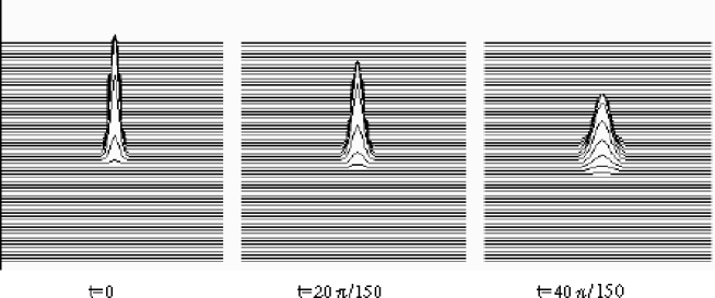
Figure 1: Evolution of a Gaussian beam with initial condition $A_{x}(x,y,z=t=0)=\exp\left(-\frac{x^{2}+y^{2}}{2}\right)$ governed by the $2D$ paraxial equation (48). The transverse size (the spot) grows approximately twice over the normalized distance $z=4\pi/15$.

7.1 Evolution of long optical pulses (light filaments)

The dynamics of optical pulses in media with week dispersion, dispersionless media and vacuum is governed by the VLAE (46). In the case of a long pulse we can express the initial conditions as follows:

$$\vec{A}=A_{x}\vec{x};\ \alpha=40;\ \delta^{2}=\frac{r_{\bot^{2}}}{z_{0}^{2}}=\frac{1}{81},$$

$$A_{x}(x,y,z,t=0)=\exp\left(-\frac{x^{2}+y^{2}+\delta^{2}z^{2}}{2}\right).$$ (79)

The solution of VLAE in a laboratory coordinate frame (6.2) for an optical pulse whose longitudinal size is nine times as large as the transverse one (7.1) is calculated by using the numerical FFT technique. The result is presented in Fig.2. The propagation distance is the same as in the previous case of a light beam $4\pi/15$. Figure 3. illustrates the spot size ($x,y$ plane) of the pulse. The analysis of the solution reveals the same evolution dynamics as in the case of an optical beam, with the diffraction length being approximately equal to the diffraction length of an optical beam $4\pi/15$. A more detailed investigation discloses the following natural dependence on the dimensionless parameters $\alpha$ and $\delta^{2}$ in the case of a long pulse: as the number of harmonics under the pulse $\alpha$ increases, together with the longitudinal size with respect to the transverse one, the VLAE solutions (6.2) approach the paraxial equation solutions (48).

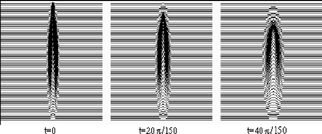
Figure 2: Evolution of a long Gaussian pulse with initial condition $A_{x}(x,y,z,t=0)=\exp\left(-\frac{x^{2}+y^{2}+\delta^{2}z^{2}}{2}\right)$, $\alpha=40;\delta=1/9$ governing by the VLAE (46). The $xz$ plane of the pulse is presented.

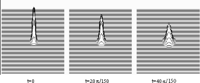
Figure 3: View of the spot, $x,y$ plane, of the same long Gaussian pulse as in Fig.2. The transverse size grows approximately twice over the same normalized distance $z=4\pi/15$ as in the case of an optical beam.

7.2 Propagation of light bullets in linear regime

The evolution of LB in media with week dispersion, dispersionless media and vacuum is governed by the same VLAE (46). The shape of the LB is symmetric in the $x$, $y$ and $z$ plane, so that the initial Gaussian profile can be written as:

$$\vec{A}=A_{x}\vec{x};\ \alpha=40;\ \delta^{2}=\frac{r_{\bot^{2}}}{z_{0}^{2}}=1,$$

$$A_{x}(x,y,z,t=0)=\exp\left(-\frac{x^{2}+y^{2}+z^{2}}{2}\right).$$ (80)

From the qualitative analysis presented in the previous section, we can expect a significant reduction of the widening of LB (of the order of $1/\delta^{2}$) with respect to long pulses or optical beams. The solution of VLAE (6.2) for LB on a distance $5\pi$, calculated again by means of the FFT technique, is illustrated in Fig.4. in the $x,z$ plane. One can only see a negligible enlargement of the pulse along a considerable distance. Figure 4. presents the solution (6.2) of the VLAE (46), with initial conditions of the type (7.2). If we consider a large distance and times $z=t>5\pi$, the LB will go out the grid. This is the reason why the next calculations of LB and LD evolution over long distances are performed in framework of the solutions (6.2) of the VLAE (47) written in a Galilean coordinate system under similar initial conditions:

$$\vec{A}=A_{x}\vec{x};\ \alpha=40;\ \delta^{2}=\frac{r_{\bot^{2}}}{z_{0}^{2}}=1,$$

$$A_{x}(x,y,z^{\prime},t^{\prime}=0)=\exp\left(-\frac{x^{2}+y^{2}+z^{\prime 2}}{2}\right).$$ (81)

The LB evolution in a Galilean frame over a long normalized distance $t=15\pi$, where the transverse width of the pulse is approximately doubled, is illustrated in Figure 5. The analytical solutions confirm the results of the qualitative analysis: the LB diffraction enlargement is significantly smaller than the enlargement of long optical pulses and optical beams. Let us remark once again that this result is only correct if the number of harmonics under the pulse, multiplied by $2\pi$, (dimensionless parameter $\alpha$) is large.

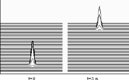
Figure 4: Evolution of a Gaussian LB under initial condition $A_{x}(x,y,z,t=0)=\exp\left(-\frac{x^{2}+y^{2}+z^{2}}{2}\right)$, $\alpha=40;\delta=1$ governed by the VLAE (46). We present the $xz$ plane of the pulse. A significantly smaller diffraction enlargement is observed, as compared with the cases of LF and light beams.

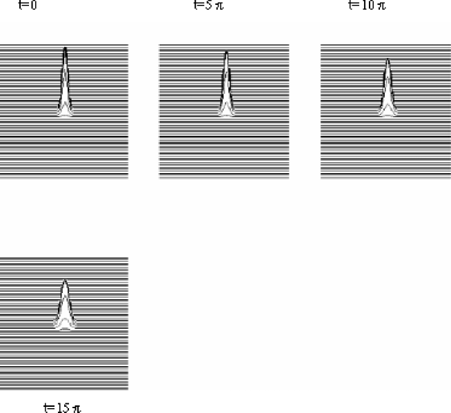
Figure 5: Evolution of the same Gaussian LB as in Fig.4 , governed now by the VLAE in a Galilean coordinate frame (47). The $xy$ plane of the pulse is presented. The LB doubles its transverse (and longitudinal) size over the normalized distance-time $t^{\prime}=z^{\prime}=15\pi$. This is approximately $10^{2}$ larger than the diffraction length of LF and light beams.

7.3 Dynamics of of light disks in linear regime. Difractionless pulses

As we mentioned in the beginning, producing optical pulses with small longitudinal and large transverse size, while at the same time keeping a large number of harmonics under the pulse, no longer presents significant experimental difficulties. This can easily be realized in the optical region for pulses with time duration from 200-300 fs up to 50-60 fs. We will again consider the propagation of LD in the framework of the solutions (6.2) of the VLAE (47) in a Galilean coordinates under initial conditions in the form:

$$\vec{A}=A_{x}\vec{x};\ \alpha=40;\ \delta^{2}=\frac{r_{\bot^{2}}}{z_{0}^{2}}=81,$$

$$A_{x}(x,y,z^{\prime},t^{\prime}=0)=\exp\left(-\frac{x^{2}+y^{2}+z^{\prime 2}}{2}\right).$$ (82)

The results of the calculations of the solutions (6.2) using FFT and inverse FFT are presented in Figure 6. Again, as one should expect bearing in mind the analysis in the previous section, the diffraction widening is practically absent. The evolution of the optical disk presented in Figure 6. demonstrates that its shape is preserved over the normalized distance and for time $t=375\pi$. This is larger by four orders of magnitude, than in the cases of diffraction of light beams and long optical pulses.

Figure 6: Evolution of an optical disk governed now by the VLAE in a Galilean coordinate frame (47). The $xy$ plane of the pulse presented. The LD preserves its shape over a distance-time $375\pi$, which is larger by $10^{4}$ than the standard diffraction length $z_{diff}=k_{0}r_{\bot}^{2}$ of light beams and long optical pulses. We call this type of optical pulses diffractionless.

This is why we refer to optical disks as being diffractionless pulses. The numerical experiments demonstrate that such pulses can propagate in media with week dispersion, in dispersionless media and in vacuum while conserving their shape over a distance of more than hundred km.

8 Conclusion

The method applied of amplitude envelopes give us the possibility to investigate and compare the propagation of optical pulses in media with strong dispersion with this in media with week dispersion, in dispersionless media and in vacuum. In the case of media with dispersion, we obtained an integro - differential nonlinear equation, describing propagation of optical pulses whose time duration is of the order of optical period of the carrier frequency, and also of pulses with many harmonics under the pulse. In the case of slowly varying amplitudes (many harmonics under the pulse) we reduced this amplitude integro - differential equation to amplitude vector nonlinear differential equations and obtained different orders of dispersion of the linear and nonlinear susceptibility. In the second case, propagation of optical pulses in dispersionless media and vacuum, we obtained an amplitude equation witch is valid in both cases, namely, pulses with many harmonics and pulses with only one-two harmonics under the envelope. We normalized these amplitude equations and obtained five dimensionless parameters determining different linear and nonlinear regimes of propagation of the optical localized waves. For optical pulses with small transverse and large longitudinal size (optical filaments) we obtained the well-known paraxial approximation, while for the case of optical pulses with a relatively equal transverse and longitudinal size (the so-called light bullets) and for the case of large transverse and small longitudinal size (light disks), we obtained new non-paraxial nonlinear amplitude equations. When the optical field is with low intensity, we reduced the nonlinear amplitude vector equation governing the evolution of LB and LD to linear amplitude equations. Surprisingly, in linear regime the normalized amplitude equations for media with dispersion and the amplitude equations in dispersionless media and vacuum are identical with accuracy of material constants. The linear equations were solved using the of Fourier transform technique. One unexpected new result is the relative stability of LB and LD and the significant reduction of the LB and LD diffraction enlargement with respect to the case of long pulses in linear regime of propagation. It is important to emphasize particularly the case of LD which are practically diffractionless over long distances exceeding hundred kilometers.

9 Acknowledgements

This work is partially supported by Bulgarian Science Foundation under grant F 1515/2005.

References

• [1] C.Ruiz, J.San Romain, C.Mendez, V.Diaz, L.Plaja, I Arias, and L.Roso Phys.Rev.Lett,95, 053905, (2005)
• [2] Y.Silberberg, Opt.Lett. 15,1282(1990).
• [3] Yu.S.Kivshar, G.P.Agrawal, Optical Solitons: From Fibers to Photonic Crystals, Academic Press, Boston,2003.
• [4] S.A. Ponomarenko, G.P.Agrawal, Opt.Comm, 261, 1-4, 2006.
• [5] R.Y.Chiao, E.Garmire and C.H.Townes, Phys. Rev. Lett. 13, 479 (1964).
• [6] V.I.Talanov, Pisma Zh. Eksp. Teor. Fiz., 2, 222 (1965).
• [7] P.L.Kelley, Phys. Rev. Lett. 15, 1005 (1965).
• [8] S.A.Akhmanov, A.P.Sukhorukov, R.V. Khokhlov, Zh. Eksp. Teor. Fiz. 50, 474 (1966).
• [9] S.A.Akhmanov, A.P.Sukhorukov, A.S.Chirkin, Zh. Eksp. Teor. Fiz. 55, 1430 (1968).
• [10] J.V.Moloney and A.C.Newell, Nonlinear Optics, (Addison-Wesley Publ. Comp.,1991).
• [11] K.L.Kovachev ”Limits of application of the slowly warrying amplitude approximation” - Bachelor Thesis, University of Sofia, 2003.
• [12] L.M.Kovachev, L.M.Ivanov, Proceedings of SPIE, 5949, Nonlinear Optics Applications, 594907-1 -594907-12, 2005.
• [13] D.N.Christodoulides, N.K.Efemidis, P.Di Trapani, B.A.Malomed, Opt.Lett., 29, 1446 (2004).
• [14] L.M.Kovachev, Int. J. of Math. and Math. Sc., 18, 949 (2004).