Oblique dark solitons in supersonic flow of a Bose-Einstein condensate

Abstract

In the framework of the Gross-Pitaevskii mean field approach it is shown that the supersonic flow of a Bose-Einstein condensate can support a new type of pattern—an oblique dark soliton. The corresponding exact solution of the Gross-Pitaevskii equation is obtained. It is demonstrated by numerical simulations that oblique solitons can be generated by an obstacle inserted into the flow.

Introduction. It is known that the nonlinear and dispersive properties of a Bose-Einstein condensate (BEC) can lead to the formation of various nonlinear structures (see, e.g., ps2003 ). Until recently, most research has been focused on experimentally observed vortices and bright and dark solitons. Furthermore, the formation of dispersive shock waves in BECs with repulsive interactions between atoms was considered theoretically in kgk04 ; damski04 and studied experimentally in rotating simula and non-rotating hoefer condensate, where it was shown that dispersive shocks are generated as a result of the evolution of large disturbances in the BEC. However, another important type of nonlinear structure, namely a spatial dark soliton, can also be realized in a BEC. The first experimental evidence of their generation has recently appeared cornell05 . In fact, the existence of oblique spatial solitons in a BEC has a natural physical basis if the Cherenkov generation of dispersive sound waves by a small obstacle in the supersonic flow of a BEC is considered and the effect of increasing the size of the obstacle (i.e. the amplitude of the waves) is determined. Evidently, along with dispersion, nonlinear effects become equally important at finite distances from the obstacle, so that the Cherenkov cone breaks-up into a spatial structure consisting of one or several dark solitons. Such a structure represents the dispersive analog of the well-known steady spatial shock generated in the supersonic flow of a viscous compressible fluid past an obstacle. In this sense, it is the spatial counterpart of the one-dimensional expanding dispersive shock kgk04 –hoefer generated in the evolution of large disturbances in a BEC. In the simplest case, the nonlinear wave structure would consist of a single spatial dark soliton given by a steady solution of the equations governing the BEC flow. Motivated by this physical consideration and the results of experiments cornell05 , in this Letter we shall develop the theory of spatial dark solitons in the framework of the Gross-Pitaevskii (GP) mean field approach.

Basic equations. The dynamics of a BEC is described to a good approximation by the GP equation ps2003

$$i\hbar\frac{\partial\psi}{\partial t}=-\frac{\hbar^{2}}{2m}\Delta\psi+V(\mathbf{r})\psi+g|\psi|^{2}\psi,$$ (1)

where $\psi({\bf r})$ is the condensate order parameter and $g$ is an effective coupling constant, with $g=4\pi\hbar^{2}a_{s}/m,$ $a_{s}$ being the $s$-wave scattering length and $m$ the atomic mass. Here $V(\mathbf{r})$ denotes the potential of the external forces acting on the condensate, for example the confining potential of the trap and/or the potential arising due to the presence of an obstacle inside the BEC. When the “obstacle” is formed by a laser beam and the flow occurs due to the free two-dimensional expansion of the BEC the trap potential should be set equal to zero for the free expansion of a BEC, and far enough from the obstacle we can neglect the obstacle potential as well. Also, we are interested in steady flows, that is, we suppose that the parameters of the flow change on a timescale much slower than the transient timescale for the establishment of the wave pattern of interest. To this end, we seek solutions of Eq. (1) with $V(\mathbf{r})=0$ of the form

$$\psi({\bf r})=\sqrt{n({\bf r})}\exp\left(\frac{i}{\hbar}\int^{{\bf r}}{{\bf u}}({\bf r}^{\prime})d{\bf r}^{\prime}\right)\exp\left(-\frac{i\mu}{\hbar}t\right),$$ (2)

where $n({\bf r})$ is the density of atoms in the BEC, ${\bf u}({\bf r})$ denotes its velocity field and $\mu$ is the chemical potential. It is now convenient to introduce the dimensionless variables $\tilde{{\bf r}}={\bf r}/\sqrt{2}\xi,\,\tilde{n}=n/n_{0},\,\tilde{\bf u}={\bf u}/c_{s},$ where $n_{0}$ is a characteristic density of atoms, equal to their density at infinity, $\xi=\hbar/\sqrt{2mn_{0}g}$ is the healing length and $c_{s}=\hbar/\sqrt{2}m\xi$ is the sound velocity in a BEC of density $n_{0}$. Substituting Eq. (2) into (1) and separating real and imaginary parts we obtain a system of equations for the density $n(x,y)$ and the two components of the velocity field ${\bf u}=(u(x,y),v(x,y))$,

$$\begin{split}(nu)_{x}+(nv)_{y}=0,\\ uu_{x}+vu_{y}+n_{x}+\left(\frac{n_{x}^{2}+n_{y}^{2}}{8n^{2}}-\frac{n_{xx}+n_{yy}}{4n}\right)_{x}=0,\\ uv_{x}+vv_{y}+n_{y}+\left(\frac{n_{x}^{2}+n_{y}^{2}}{8n^{2}}-\frac{n_{xx}+n_{yy}}{4n}\right)_{y}=0,\end{split}$$ (3)

where we have omitted tildes for convenience. If we restrict our consideration to the vortices-free potential flows with vanishing curl of the velocity field,

$$u_{y}-v_{x}=0,$$ (4)

then the second and third equations in (3) can be integrated once to give a generalization of the Bernoulli theorem to dispersive 2D hydrodynamics:

$$\frac{1}{2}(u^{2}+v^{2})+n+\frac{1}{8n^{2}}(n_{x}^{2}+n_{y}^{2})-\frac{1}{4n}(n_{xx}+n_{yy})=\mathrm{const}.$$ (5)

Equations (4), (5) and the first equation of (3) comprise the system governing the BEC potential flow.

Our aim now is to find the solution of this system under the conditions that the BEC flow is uniform at infinity

$$n=1,\quad u=M,\quad v=0\quad\text{at}\quad|x|\to\infty,$$ (6)

where $M$ denotes the ratio of the asymptotic velocity of the flow to the sound velocity, i.e. the Mach number.

Oblique dark soliton solution. Let us seek a solution of the form $n=n(\theta)$, $u=u(\theta)$, $v=v(\theta)$, where $\theta=x-ay$ and $a$ denotes the slope of the soliton center location with the $y$ axis. Substitution of this ansatz  into (4) and the first equation of (3), followed by a simple integration, yields expressions for the velocity components in terms of the density

$$u=\frac{M(1+a^{2}n)}{(1+a^{2})n},\quad v=-\frac{aM(1-n)}{(1+a^{2})n},$$ (7)

where the integration constants were chosen according to condition (6). Then substitution of (7) into (5), with a proper choice of the constant in the right-hand side, leads to the equation

$$\tfrac{1}{4}(1+a^{2})(n_{\theta}^{2}-2nn_{\theta\theta})+2n^{3}-(2+p)n^{2}+p=0,$$ (8)

where

$$p=M^{2}/(1+a^{2}).$$ (9)

It is easily checked that Eq. (8) has the integral

$$\tfrac{1}{4}(1+a^{2})n_{\theta}^{2}=(1-n)^{2}(n-p)$$ (10)

where, again, the integration constant is chosen in accordance with condition (6). Simple integration of this equation finally yields the desired solution in the form of a dark soliton for the density

$$n(\theta)=1-\frac{1-p}{\cosh^{2}[\sqrt{1-p}\,\theta/\sqrt{1+a^{2}}]}.$$ (11)

The velocity components can then be found by substitution of this solution into Eqs. (7). The inverse half-width of the soliton in the $x$-direction is

$$\kappa=2\sqrt{\frac{1-p}{1+a^{2}}}.$$ (12)

Thus formulae (11) and (12) give the exact dark spatial soliton solution of the GP equation. We shall call it “oblique” because it is always inclined with respect to the direction of the supersonic flow. Numerical solutions below show that such solutions are stable for $M>1$.

Small amplitude Korteweg-de Vries (KdV) limit. As is clear from (11) the small amplitude limit is achieved when $1-p\ll 1$. Then the parameters $a$ and $p$ can be expressed in terms of $\kappa$ and $M$ from Eqs. (9) and (12) as

$$a\cong\sqrt{M^{2}-1}+\frac{M^{4}\kappa^{2}}{8\sqrt{M^{2}-1}},\quad 1-p\cong\frac{1}{4}\kappa^{2}M^{2}.$$ (13)

The density profile in this limit becomes then familiar KdV soliton

$$n\cong 1-\frac{M^{2}\kappa^{2}}{4\cosh^{2}[\kappa(x-ay)/2]},$$ (14)

where $\kappa\ll 1/M$.

Note that the slope $a=\sqrt{M^{2}-1}$ corresponds exactly to the Cherenkov cone, so that in its vicinity the small amplitude solitons are located inside it. This approximation corresponds to the KdV limit of the potential-free GP equations (3). Indeed, if we assume the series expansions $(\varepsilon\ll 1)$

$$n=1+\varepsilon n_{1}+\ldots,\quad u=M+\varepsilon u_{1}+\ldots,\quad v=\varepsilon v_{1}+\ldots$$ (15)

and introduce the scaling of the independent variables $\zeta=\varepsilon^{1/2}(x-ay),\quad\tau=\varepsilon^{3/2}y$, then standard reductive perturbation theory leads to the KdV equation for the density disturbance $n_{1}$

$$\partial_{\tau}n_{1}-\frac{3M^{2}}{2\sqrt{M^{2}-1}}n_{1}\partial_{\zeta}n_{1}+\frac{M^{4}}{8\sqrt{M^{2}-1}}\partial^{3}_{\zeta\zeta\zeta}n_{1}=0,$$ (16)

with the well-known soliton solution of this equation equivalent to (14), (13).

Nonlinear Schrödinger (NLS) equation limit. Another important limit corresponds to large slopes $a^{2}\gg 1$. For this limit we introduce the parameter $\lambda$ as $p\cong M^{2}/a^{2}=\lambda^{2}$, that is $a=\pm M/\lambda$. The soliton solution (11) can then be approximated as

$$n\cong 1-\frac{1-\lambda^{2}}{\cosh^{2}[\sqrt{1-\lambda^{2}}(y\pm\lambda x/M)]}.$$ (17)

This is exactly the solution $n=|\Psi|^{2}$ of the NLS equation

$$i\Psi_{T}+\Psi_{YY}-2|\Psi|^{2}\Psi=0$$ (18)

for the complex variable $\Psi=\sqrt{n}\exp\left(i\int^{Y}v(Y^{\prime},t)dY^{\prime}\right)$, where $T=x/2M$ and $Y=y$. This equation was derived in ek-pla06 from the GP equations (3) for the highly supersonic ($M\gg 1$) flow of a BEC past a slender body.

Generation of oblique solitons in a BEC. Let us now consider the supersonic flow of a BEC past an obstacle. If the obstacle is small (e.g. an impurity), then linear sound waves are generated at finite distances which form a Cherenkov cone AP04 . Large obstacles generate spatial dispersive shocks which can be viewed as trains of interacting dark spatial solitons inside the Cherenkov cone. The theory of the generation of spatial dispersive shocks has been developed in much detail for supersonic flows past a slender body when such a flow can be described by the KdV equation GKKE95 . Analogous theory for the NLS equation case was developed in ek-pla06 . However, in real experiments the obstacles cannot be considered as slender bodies and the flow is not highly supersonic, hence fully nonlinear solutions of the GP equation, such as Eq. (11), should be used for the quantitative description of spatial dispersive shocks in a BEC. Here we shall use numerical solutions of the GP equation to demonstrate that the structures generated by an obstacle inserted into the supersonic BEC flow indeed contain the oblique dark solitons given by Eq. (11).

To make this process clearer, numerical solutions of the time-dependent GP equation (1), expressed in non-dimensional variables as

$$i\psi_{t}=-\frac{1}{2}(\psi_{xx}+\psi_{yy})+V(x,y)\psi+|\psi|^{2},$$ (19)

were studied, where $\widetilde{\psi}=\psi/\sqrt{n_{0}}$ and $\tilde{t}=(gn_{0}/\hbar)t$, with the other variables defined as in Eq. (2). From now on, the tildes will be omitted. The potential $V(x,y)$ corresponds to the interaction of the condensate with the obstacle. Since the detailed behavior of the potential should not be critical for the formation of solitons far from the obstacle, it can be safely modeled by an impenetrable disk. In our simulations its radius was set to $r=1$ in our non-dimensional units. Initially at $t=0$ there is no disturbance in the condensate, so that it is described by the plane wave function $\left.\psi(x,y)\right|_{t=0}=\exp(iMx)$ corresponding to a uniform condensate flow. To be specific, let us take $M=5$. Several stages of the numerically calculated BEC density evolution are shown in Fig. 1.

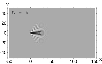
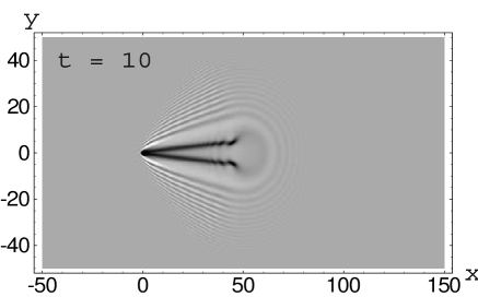
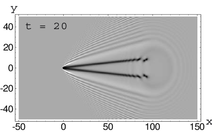
Figure 1: Emergence of a pair of oblique dark solitons after “switching on” supersonic flow ($M=5$) past a disk-shaped impenetrable obstacle of radius $r=1$ located at $(x=0,y=0)$. The direction of the flow is from left to right. Density plots are shown for three times $t=5$, $t=10$ and $t=20$. The dark structures correspond to oblique dark solitons, which in turn generate the vortex streets near the end points.

It can be clearly seen how a pair of oblique solitons is gradually formed behind the obstacle. Their length grows with time and, except in the vicinity of the end points, the density distributions do not demonstrate any vorticity, which agrees with our assumption of potential flow (4). However, the flow cannot be considered as stationary and potential near the end points. This is manifested by the presence of vortices behind the end points of the spatial solitons. One may interpret these vortices as a “vortex street” WMCA radiated by spatial dark solitons. However far enough away from these vortex end points, the flow can be considered stationary. The establishment time of the stationary profile can be estimated by the soliton width divided by the sound velocity, which is $t\sim 2$ in our solutions. This is much less than the value $t=20$ for the last plot of Fig. 1. The parameter $p$ from Eq. (9) was calculated using the value of the slope $a$ inferred from the numerical solution. A comparison of the theoretical profile of the oblique dark soliton given by Eq. (11) with the corresponding part of the density profile in the full numerical solution is shown in Fig. 2. The excellent agreement between these two profiles confirms that the line patterns in Fig. 1 are indeed oblique dark solitons generated by the obstacle. This agreement also justifies the assumptions made in the derivation of the analytic solution (11). Note that, along with the soliton, a small amplitude dispersive wave packet is generated, which corresponds to the “non-solitonic” part of the density perturbation induced by the obstacle. This wave packet spreads out as distance from the obstacle increases and eventually fades away.

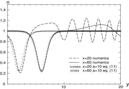
Figure 2: Cross sections of the density distributions for $x=20$ (dashed line), $x=60$ (solid line) and $y>0$ obtained from numerical solution of the GP equation (19). These are compared with soliton profiles (11) with slope $a=10$ shown as functions of $y$ at the same values of $x$ ($x=20$ corresponds to “crosses” and $x=60$ to “circles”).

In the above simulations, the parameters of the obstacle have been chosen so that only a single soliton is generated at each side of the obstacle. However, with the increase of the size $r$ of the obstacle the number of solitons is also expected to increase. This effect is demonstrated in Fig. 3 in which two symmetric fans of solitons can be seen behind the obstacle. As expected, the depth of the dark solitons grows with the increase of the slope $a$ with respect to the $y$ axis. Thus, the oblique dark solitons can be viewed as “building blocks” in more complicated patterns arising in supersonic flows of a BEC. This figure also demonstrates the robustness of the phenomenon for different obstacle parameters. The whole structure in Fig. 3 represents a pair of dispersive shocks generated in the supersonic flow of a BEC past an obstacle. Such shocks were considered in ek-pla06 in the limiting case of highly supersonic flow ($M\gg 1$) and slender obstacles ($a\gg 1$). Our present numerical simulations show that spatial dispersive shocks represent a general phenomenon caused by the interplay of dispersive and nonlinear effects described by the full GP equation. We speculate that it can be also be observed in flows of a BEC past 3D obstacles.

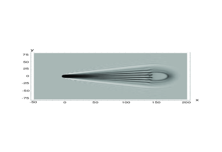
Figure 3: Density plot at the moment $t=30$ for the supersonic flow ($M=5$) past a disk-shaped impenetrable obstacle with radius $r=5$ located at $(x=0,y=0)$.

The above theory is based on the supposition that the flow of a BEC is homogeneous and uniform enough for periods of time sufficient for generation of oblique dark solitons. Let us indicate here the physical conditions which should be satisfied for obtaining such a flow in experiment. To be definite, we consider the example of 2D flow in “pancake” geometry, that is the condensate is supposed to be confined in axial direction by a strong harmonic potential. Let the transversal frequency $\omega_{\bot}$ of the potential be small enough so that the (radial) Thomas-Fermi density distribution is applicable. We consider expansion of the BEC after switching off the potential (see, e.g. kam04 ). The asymptotic as $t\gg 1/\omega_{\bot}$ solution of the cylindric GP equation for $r\ll l\omega_{\bot}t$ where $l$ is the radius of the BEC before its release from the trap, is given by $n(r,t)\cong{\hbox{constant}}/({\omega_{\bot}t})^{2}$, $u(r,t)\cong{r}/t$, that is the density is practically uniform but varying with time. In the same approximation, the local healing length $\xi$ and the local sound velocity $c_{s}$ are given by $\xi={\hbar t}/{ml},$ $c_{s}={l}/({\sqrt{2}t})$. Hence, the local Mach number $M\cong{\sqrt{2}r}/{l}.$ Thus, we get a supersonic flow past obstacle if we place it at the distance $d>l/\sqrt{2}$ from the axis. Now, the flow can be considered as uniform if the size of the obstacle (scaled as healing length $\xi$ for a chosen moment of observation) satisfies the condition $\xi/d\ll 1$. For $d\sim l$ this gives $t\ll{ml^{2}}/{\hbar}$, i.e the flow past an obstacle is asymptotically uniform for $\omega_{\bot}^{-1}\ll t\ll{ml^{2}}/{\hbar}$. At last, the characteristic time of establishing the soliton distribution, ${\xi}/{c_{s}}\sim{m\xi^{2}}/{\hbar}$, obviously satisfies the above inequality since $\xi\ll l$, so that the flow can be considered as quasi-stationary. At the same time, our numerical simulations show that oblique solitons are generated even in non-uniform and nonhomogeneous flows past obstacles, that is the phenomenon is very robust with respect to change of parameters of the flow.

To summarize, we have found an exact oblique dark soliton solution of the GP equation and demonstrated numerically that such solitons can be generated by obstacles inserted into the supersonic flow of a BEC.

AMK thanks EPSRC and RFBR (grant 05-02-17351) and AG thanks FAPESP and CNPq for financial support.

References

- (1) L.P. Pitaevskii and S. Stringari, Bose-Einstein Condensation, (Cambridge University Press, Cambridge, 2003).
- (2) A.M. Kamchatnov, A. Gammal, and R.A. Kraenkel, Phys. Rev. A 69, 063605 (2004).
- (3) B. Damski, Phys.Rev. A 69, 043610 (2004).
- (4) T.P. Simula et al., Phys. Rev. Lett. 94, 080404 (2005).
- (5) M.A. Hoefer et al, preprint cond-mat/0603389.
- (6) E.A. Cornell, talk at “Conference on Nonlinear Waves, Integrable Systems and their Applications”, (Colorado Springs, June 2005); available at http://jilawww.colorado.edu/bec/papers.html.
- (7) G.A. El and A.M. Kamchatnov, Phys. Lett A 350, 192 (2006); erratum: Phys. Lett. A 352, 554 (2006).
- (8) G.E. Astrakharchik and L.P. Pitaevskii, Phys. Rev. A 70, 013608 (2004).
- (9) A.V. Gurevich, A.L. Krylov, V.V. Khodorovskii, and G.A. El, JETP, 81, 87 (1995); 82, 709 (1996).
- (10) T. Winiecki, J.F. McCann, and C.S. Adams, Phys. Rev. Lett. 82, 5186 (1999).
- (11) A.M. Kamchatnov, JETP 94, 908 (2004).