Coexistence of Josephson oscillations and novel self-trapping regime in optical waveguide arrays

Abstract

Considering the coherent nonlinear dynamics between two weakly linked optical waveguide arrays, we find the first example of coexistence of Josephson oscillations with a novel self-trapping regime. This macroscopic bistability is explained by proving analytically the simultaneous existence of symmetric, antisymmetric and asymmetric stationary solutions of the associated Gross-Pitaevskii equation. The effect is, moreover, illustrated and confirmed by numerical simulations. This property allows to conceive an optical switch based on the variation of the refractive index of the linking central waveguide.

Introduction.

Since its prediction joseph in 1962 and the immediate experimental verification anderson , the Josephson effect has led to many implementations in various branches of physics. This macroscopic quantum tunneling effect, originally discovered in superconducting junctions, is caused by the global phase coherence between electrons in the different layers. Similar Josephson oscillations have been discovered in liquid Helium helium1 ; helium2 and in double layer quantum Hall systems hall1 ; hall2 .

The first realization of a bosonic Josephson junction has been recently experimentally reported ober for a Bose-Einstein condensate embedded in a macroscopic double well potential. The difference of the latter from the ordinary Josephson junction behavior is that the oscillations of population imbalance are suppressed for high imbalance values and a self-trapping regime emerges smerzi1 ; smerzi2 . The optical realization of a bosonic junction had been theoretically proposed much earlier by Jensen jensen who considered light power oscillations in two coupled nonlinear waveguides.

In order to describe the macroscopic tunneling effect in bosonic junctions, the nonlinear dynamics is usually mapped to a simpler system characterized by two degrees of freedom (population imbalance and phase difference) while the nonlinear properties of the wave function within the single well are neglected. In this approach the symmetric and antisymmetric stationary solutions of the Gross-Pitaevskii equation gros are used as a basis to build a global wave function kivshar1 ; ananikian . In the weakly nonlinear limit this description is fully valid because those symmetric and antisymmetric functions are the only solutions of the equation. For higher nonlinearities an asymmetric stationary solution appears, which represents a novel self-trapping state alberto .

In this Letter, we consider the two weakly linked optical waveguide arrays represented in Fig. 1. When light is mainly injected in one array (e.g. the right one, as shown in Fig.1), we find a wide light intensity range where it can either remain trapped in this array, or swing periodically from right to left and back. The switching from one state to the other is determined by a slight variation of the refractive index of the central linking waveguide denoted with the index 0. The coexistence of the oscillatory and self-trapping regimes corresponds to the simultaneous presence of Josephson oscillation states and asymmetric solutions of the Gross-Pitaevskii equation. This is in contrast with all known behaviors of bosonic Josephson junctions, where the existence of oscillatory and self-trapping regimes is uniquely determined by the parameters of the system. Our theoretical result is expected to have a straightforward experimental realization in waveguide arrays and in Bose-Einstein condensates with double well potential.

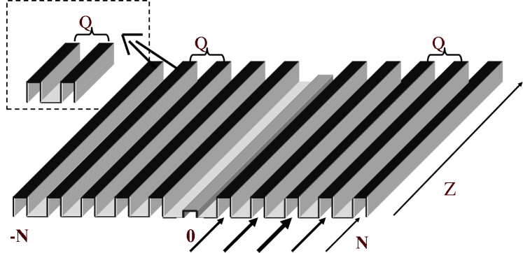
Figure 1: Scheme of the proposed setup of two weakly linked waveguide arrays. The refractive index of the central waveguide is smaller than the indices of the waveguides in the two arrays. The inset displays the elementary cell with the coupling constant $Q$.

The model.

Waveguide arrays are particularly convenient for a direct observation of nonlinear effects, because the longitudinal dimension $z$ plays the role of time. With an intensity-dependent refractive index (optical Kerr effect), waveguide arrays become soliton generators, as experimentally demonstrated in eisenberg ; morandotti ; mandelik ; yuri ; fleisher1 ; fleisher2 ; assanto1 .

The model of an array of adjacent waveguides coupled by radiation power exchange is the Discrete NonLinear Schrödinger equation (DNLS) christ-joseph ; mark and nonlinearity then manifests itself by a self-modulation of the input signal (injected radiation). It reads

$$i\frac{\partial\psi_{j}}{\partial z}+\frac{\omega}{c}n_{j}\psi_{j}+Q\bigl{(}\psi_{j+1}+\psi_{j-1}-2\psi_{j}\bigr{)}+|\psi_{j}|^{2}\psi_{j}=0,$$ (1)

where waveguides discrete positions are labelled by the index $j$ ($-N\leq j\leq N$), and complex light amplitudes $\psi_{j}$ are normalized such as to fix the onsite nonlinearity to the unitary value. The linear refractive index $n_{j}$ is set to $n$ for all $j\neq 0$, and to $n_{0}<n$ for $j=0$. The coupling constant between two adjacent waveguides is $Q$ and $\omega$ and $c$ are the frequency and the velocity of the injected light, respectively. Last, we assume vanishing boundary conditions $\psi_{N+1}=\psi_{-N-1}=0$ in order to mimick a strongly evanescent field outside the waveguides.

The above equation, written for two waveguides (elementary cell in the inset of Fig.1), straightforwardly reduces to the one considered by Jensen jensen . In that case the resulting dynamics is given in terms of Jacobi elliptic functions  jensen ; smerzi2 and can be described as follows. For a beam of small intensity, light tunnels from one waveguide to the other and then back, inducing Josephson oscillations. Indeed, the elementary cell is similar to a single bosonic Josephson junction as demonstrated in smerzi1 ; smerzi2 and experimentally observed in Bose-Einstein condensates ober . Increasing the injected beam intensity above some critical value, light becomes self-trapped and does not tunnel to the other waveguide, which constitutes the difference between a bosonic Josephson junction and its superconducting analogue.

Numerical simulations.

We demonstrate now by numerical simulations of model (1) that for the device of Fig.1, the two regimes, namely Josephson oscillations and self-trapping, coexist for a given injected beam intensity and given parameter values. The switch from one state to the other is achieved, for instance, by a tiny local variation of the refractive index of the central waveguide.

Let us choose the following values for the parameters in equation (1):

$$N=14,\quad Q=16,\quad V_{0}\equiv\omega(n-n_{0})/2c=10,$$ (2)

together with the following input light envelope

$$\psi_{j}(0)=0.4\,\sin\bigl{[}(j-N-1)/5.5\bigr{]},\quad j=1,\cdots N,$$ (3)

$$\psi_{j}(0)=0.2\,\sin\bigl{[}(j+N+1)/5.5\bigr{]},\quad j=-N,\cdots 0,$$

which represents a beam mostly sent into the right waveguide array. Figure 2 displays the result of our numerical simulations. While the relative refractive index $V_{0}$ of the central waveguide is kept constant, the power injected initially into the right part of the array remains self-trapped, as shown in Fig.2 up to $z=150$. A local variation of $V_{0}$ at $z=150$, as drawn in the inset of Fig.2, makes the self-trapping state bifurcate to a regime of Josephson oscillations, which then remains stable.

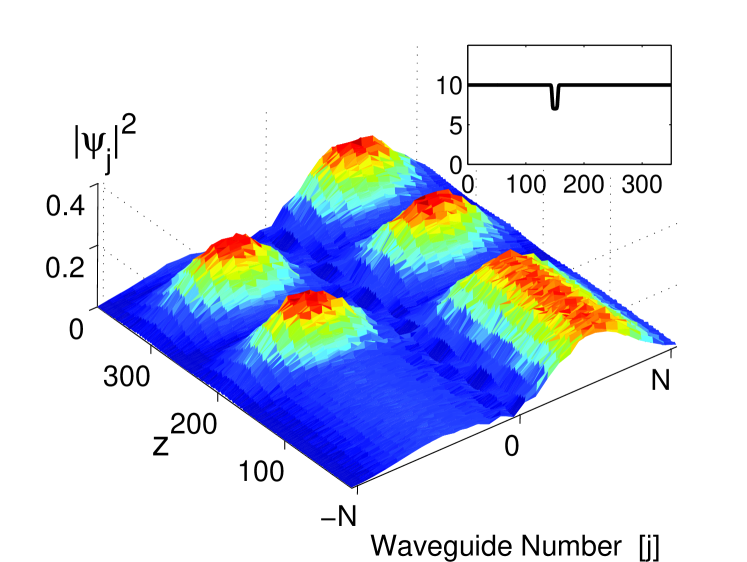
Figure 2: Numerical simulation of the DNLS equation (1) with $z=0$ initial conditions (3) and parameters (2). By a slight local variation at $z=150$ of the refractive index of the central waveguide (represented in the inset in terms of the relative barrier height $V_{0}$), the regime switches from self-trapping to Josephson oscillations. The injected total power is $P_{t}=\sum|\psi_{j}|^{2}=1.7$.

Theory.

We shall now interpret these results in terms of the continuum limit of model (1), which, after an appropriate phase shift, reads as the Gross-Pitaevskii equation

$$i\frac{\partial\psi}{\partial z}+\frac{\partial^{2}\psi}{\partial x^{2}}-V(x)\psi+|\psi|^{2}\psi=0.$$ (4)

The wavefunction $\psi(z,x)$ depends on the spatial continuous variables $z$ and $x=j/\sqrt{Q}$. $V(x)$ is a double well potential with a width $2L=(2N+2)/\sqrt{Q}$ and is represented in Fig. 3. The potential barrier of the double well potential has height $V_{0}$ and width $2l=1/\sqrt{Q}$. In the region of the barrier we assume, for technical simplification, that the Schrödinger equation can be treated in the linear approximation, while numerical simulations are performed with a fully nonlinear array. The stationary solution of (4) are sought as $\psi(z,x)=\Phi(x)\exp(-i\beta z)$, where the real-valued function $\Phi(x)$ is found in terms of Jacobi elliptic functions as follows book :

$$-l<x<-L\ :\ \Phi=B\ {\rm cn}[\gamma_{B}(x+L)-{\mathbb{K}}(k_{B}),k_{B}],$$

$$-l<x<l\ :\ \Phi=ae^{\lambda x}+be^{-\lambda x},$$ (5)

$$l<x<L\ :\ \Phi=A\ {\rm cn}[\gamma_{A}(x-L)+{\mathbb{K}}(k_{A}),k_{A}],$$

with the constants

$$\gamma_{A}=\sqrt{A^{2}+\beta},\quad\gamma_{B}=\sqrt{B^{2}+\beta},\quad\lambda=\sqrt{V-\beta},$$ (6)

${\mathbb{K}}$ denotes the complete elliptic integral of the first kind and the moduli are

$$k_{A}^{2}=\frac{A^{2}}{2(A^{2}+\beta)},\quad k_{B}^{2}=\frac{B^{2}}{2(B^{2}+\beta)}.$$ (7)

The above solutions are given in terms of five parameters ($A$, $B$, $a$, $b$, $\beta$). As the continuity conditions at points $x=\pm l$ provide four relations, the total injected power $P_{t}=\int|\psi|^{2}dx$ completely determines the solutions.

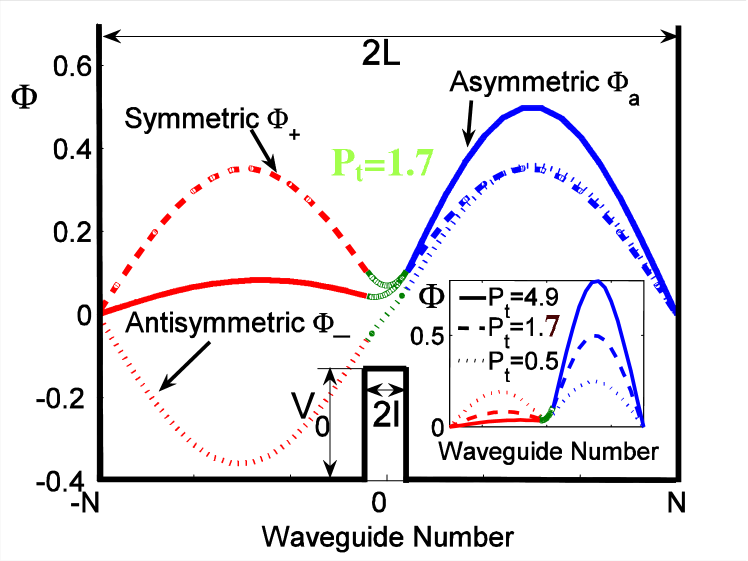
Figure 3: Plot of the double well potential for the continuous model (4): $2L$ is the well width, $V_{0}$ and $2l$ are barrier height and width. The curves are the plots of different types of solutions for the total power $P_{t}=1.7$. The inset shows the form of the asymmetric solution for different values of the total power.

In the weakly nonlinear limit $P_{t}\ll 1$, the solutions are either symmetric or antisymmetric. The even solution $\Phi_{+}(x)$ corresponds to $A=B$ in (5) when the solution in the barrier region is $2a\cosh(\lambda x)$. The odd solution $\Phi_{-}(x)$ corresponds to $A=-B$ with central solution $2a\sinh(\lambda x)$. For higher powers, namely above a threshold value, an asymmetric solution $\Phi_{a}(x)$ also exists for which $A\neq\pm B$. These analytical solutions are represented in Fig. 3.

Using the symmetric and antisymmetric basic solutions, one can build a variational anzatz following kivshar1 ; ananikian by seeking the solution $\psi(z,x)$ under the form

$$\psi(z,x)=\psi_{1}(z)\Phi_{1}(x)+\psi_{2}(z)\Phi_{2}(x),$$ (8)

$$\Phi_{1}=\frac{1}{\sqrt{2}}(\Phi_{+}+\Phi_{-}),\quad\Phi_{2}=\frac{1}{\sqrt{2}}(\Phi_{+}-\Phi_{-}).$$

The functions $|\psi_{1}|^{2}$ and $|\psi_{2}|^{2}$ are interpreted as the probabilities to find the light localized on the left or right array. By construction, the overlap of $\Phi_{1}$ with $\Phi_{2}$ is negligible, namely

$$\int\Phi_{1}\Phi_{2}dx\ll\int dx\ \Phi_{1}^{2}=\int dx\ \Phi_{2}^{2},$$ (9)

where the integrals run on $x\in[-L,L]$. Consequently, the projection of the Gross-Pitaevskii equation (4) on $\Phi_{1}$ and $\Phi_{2}$ provides the coupled mode equations jensen ; smerzi1

$$i\frac{\partial\psi_{1}}{\partial z}-E_{1}\psi_{1}+D|\psi_{1}|^{2}\psi_{1}=r\psi_{2},$$

$$i\frac{\partial\psi_{2}}{\partial z}-E_{2}\psi_{2}+D|\psi_{2}|^{2}\psi_{2}=r\psi_{1},$$ (10)

with coupling constant $r$ and nonlinearity parameter $D$ defined by

$$r=\frac{\int\left[(\partial_{x}\Phi_{1})(\partial_{x}\Phi_{2})+V\Phi_{1}\Phi_{2}\right]dx}{\int\Phi_{1}^{2}\,dx},\quad D=\frac{\int\Phi_{1}^{4}\,dx}{\int\Phi_{1}^{2}\,dx}.$$

The linear levels $E_{1}$ and $E_{2}$ are given by

$$E_{n}=\frac{\int\left[(\partial_{x}\Phi_{n})^{2}+V\Phi_{n}^{2}\right]dx}{\int\Phi_{n}^{2}\,dx},\quad n=1,2,$$ (11)

and turn out to be equal thanks to (9). As a consequence they can be absorbed in a common phase in (10).

An explicit solution of (10) in terms of Jacobi elliptic functions has been found in jensen and used in Bose-Einstein condensates in smerzi2 . It has a simple form when all the power is initially injected into one array, say $|\psi_{1}(0)|=1$, $|\psi_{2}(0)|=0$. Solutions have different behavior depending on the value of $D$ being below or above the threshold value $4r$

$$D<4r\ : \ |\psi_{1}(z)|^{2}=\frac{1}{2}\left[1+{\rm cn}(2rz,\frac{D}{4r})\right],$$ (12)

$$D>4r\ : \ |\psi_{1}(z)|^{2}=\frac{1}{2}\left[1+{\rm dn}(\frac{D}{2}z,\frac{4r}{D})\right].$$ (13)

with $|\psi_{2}|^{2}=1-|\psi_{1}|^{2}$. Solution (12) describes an oscillation of light intensity between the left and the right array (Josephson regime), since $|\psi_{1}|$ oscillates around the value $0$. The period of this oscillation is

$$T=2{\mathbb{K}}(D/4r)/r.$$ (14)

For $D>4r$ solution (13) oscillates around the value $1/2+1/4(1+\sqrt{1-(4r/D)^{2}})$ with a period

$$T^{\prime}=8{\mathbb{K}}(4r/D)/D,$$ (15)

which shows that the system is in the self-trapping regime. Such simple explicit formulas provide two important informations on the response of the system to irradiation of one array, namely the period of the Josephson oscillations and the threshold (in terms of parameter $D$) above which we expect a bifurcation to a self-trapping regime.

However, the picture of possible solutions is not yet complete. We discuss here the appearance of a further asymmetric solution when the injected power exceeds a smaller threshold value. To be definite, we restrict to the parameter values which follow from (2): the width of the double well potential is $2L=7.5$, the barrier width is $2l=0.25$ and its height is $V_{0}=10$. We derive the complete set of solutions (5) and display the dependence of their amplitudes on the total power $P_{t}=\int|\psi|^{2}dx$ in the main plot of Fig.4. Below the smaller threshold value $P_{t}=0.76$ (showed by the vertical bold dashed line) only the symmetric and antisymmetric solutions exist and their amplitudes almost superpose. At this threshold value a new solution appears which is asymmetric and the amplitudes in the two arrays are represented by the upper ($U$) and lower ($L$) branch in Fig. 4. The existence of this solution is at the basis of a novel self-trapping regime as we explain below. At a bigger threshold value (indicated by the vertical dotted line) solution (8) changes from the Josephson regime to the usual self-trapping one described above.

In the region of injected power where the asymmetric solution coexists with the symmetric and asymmetric stationary solutions one can induce flipping of one to the other by varying the height of the barrier as shown in Fig. 2. It is likely that one can induce such flips by other methods (e.g. by the variation of the profile of the injected power).

Going back to Josephson oscillations related to the symmetric and antisymmetric solutions, a simple striking numerical check is provided by the inset of Fig. 4, where we plot the period of the oscillation against the injected power. Numerical data, which are obtained with the fully discrete (and fully nonlinear) model (1) for parameters in (2), compare extremely well with (14).

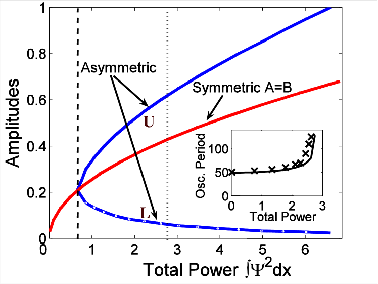
Figure 4: Main plot: dependence of the amplitudes (maximum values on $x\in[-L,L]$) of the symmetric and asymmetric solutions (5) on the total power (we have not reported the amplitude of the antisymmetric solution which almost superposes to the one of the symmetric). The inset displays the period of the Josephson oscillations for various values of the injected power: the full line corresponds to the analytical expression (14), the crosses are results of numerical simulations.

In conclusion a new coherent state in weakly linked waveguide arrays has been discovered. This coherent state has the property of being bistable and one can easily switch from oscillatory to self-trapping regimes and back. This nontrivial behavior may have interesting applications in various weakly linked extended systems, such as Bose-Einstein condensates or Josephson junctions arrays, which deserve further studies.

References

- (1) B. D. Josephson, Phys. Lett. 1, 251 (1962).
- (2) P.L. Anderson, J.W. Rowell, Phys. Rev. Lett. 10, 230 (1963).
- (3) S.V. Pereverzev, A. Loshak, S. Backhaus, J. C. Davis, R. E. Packard, Nature, 388, 449 (1997).
- (4) K. Sukhatme, Y. Mukharsky, T. Chui, D. Pearson, Nature, 411, 280 (2001).
- (5) I.B. Spielman et. al., Phys. Rev. Lett., 84, 5808, (2000), ibid. 87, 036803 (2001).
- (6) M.M. Fogler, F. Wilczek, Phys. Rev. Lett., 86, 1833, (2001).
- (7) M. Albiez, R. Gati, J. Folling, S. Hunsmann, M. Cristiani, M. K. Oberthaler, Phys. Rev. Lett., 95, 010402 (2005).
- (8) A. Smerzi, S. Fantoni, S. Giovanazzi, S. R. Shenoy, Phys. Rev. Lett., 79, 4950 (1997).
- (9) S. Raghavan, A. Smerzi, S. Fantoni, S. R. Shenoy, Phys. Rev. A, 59, 620 (1999).
- (10) S.M. Jensen, IEEE J. Quantum Electron. 18, 1580, (1982).
- (11) L. P. Pitaevskii, Sov. Phys. JETP, 13, 451, (1961); E. P. Gross, Nuovo Cimento, 20, 454, (1961); J. Math. Phys., 4, 195, (1963).
- (12) E. A. Ostrovskaya et. al., Phys. Rev. A, 61, 031601(R), (2000).
- (13) D. Ananikian, T. Bergeman, Phys. Rev. A, 73, 013604, (2006).
- (14) A. Montina, F.T. Arecchi, Phys. Rev. A, 66, 013605, (2002).
- (15) H.S. Eisenberg et. al., Phys. Rev. Lett., 81, 3383, (1998).
- (16) R. Morandotti, H.S. Eisenberg, Y. Silberberg, M. Sorel, J.S. Aitchison, Phys. Rev. Lett., 86, 3296, (2001).
- (17) D. Mandelik et. al., Phys. Rev. Lett., 90, 053902, (2003); Phys. Rev. Lett., 92, 093904, (2004).
- (18) A.A. Sukhorukov, D. Neshev, W. Krolikowski, Y.S. Kivshar, Phys. Rev. Lett., 92, 093901, (2004).
- (19) J.W. Fleischer et al., Phys. Rev. Lett., 90, 023902, (2003).
- (20) J.W. Fleischer et al., Nature, 422, 147, (2003).
- (21) A. Fratalocchi, G. Assanto, Phys. Rev. E 73, 046603 (2006); A. Fratalocchi et. al., Opt. Express, 13, 1808, (2005).
- (22) D.N. Christodoulides, R.I. Joseph, Optics Lett., 13, 794, (1988).
- (23) M.J. Ablowitz, Z.H. Musslimani, Phys. Rev. Lett. 87, 254102, (2001); Phys. Rev. E, 65, 056618, (2002).
- (24) P.F. Byrd, M.D. Friedman, Handbook of elliptic integrals for engineers and physicists, Springer (Berlin 1954).