Universal Scaling Laws for Large Events in Driven Nonequilibrium Systems

Abstract

For many driven-nonequilibrium systems, the probability distribution functions of magnitude and recurrence-time of large events follow a powerlaw indicating a strong temporal correlation. In this paper we argue why these probability distribution functions are ubiquitous in driven nonequilibrium systems, and we derive universal scaling laws connecting the magnitudes, recurrence-time, and spatial intervals of large events. The relationships between the scaling exponents have also been studied. We show that the ion-channel current in Voltage-dependent Anion Channels obeys the universal scaling law.

The physics of nonequilibrium systems has been of major interest in last several decades. Recently large events have become a major resource for characterizing nonequilibrium system. Bak et al. Bak et al. (1987, 1988) constructed a model called “sandpile” to abstract some of the essential features of driven-nonequilibrium systems. Original model of Bak et al. (BTW) as well as its variants exhibit powerlaw behaviour for the magnitude and duration of avalanches, which play the role of large events. Later scientists started investigating the temporal correlations in various systems using recurrence-time pdf of large events. In the BTW model, the pdf of recurrence time ($\tau$) of large events is $\exp(-\tau/\tau_{c})/\tau_{c}$, which indicates that the triggering of large events in this system are uncorrelated Boffetta et al. (1999); Sánchez et al. (2002). This is a generic feature of Poisson process. It was however soon realized that the events are correlated in many nonequilibrium systems. Boffatta et al. Boffetta et al. (1999) studied solar flares, and found that the pdf of recurrence time for the solar flares is a powerlaw, i. e.,

$$P(\tau)=A\tau^{-\beta},$$ (1)

with $\beta\approx 2.4$. These authors also studied the recurrence-time distribution for the dissipation-bursts in magnetohydrodynamic turbulence, and again found a powerlaw with $\beta\sim 2.7$. These results show that the large events in solar flares and magnetohydrodynamic turbulence are temporally correlated. Note that the pdf of solar-flare magnitudes is a powerlaw just like sandpile model Lu and Hamilton (1991); Baiesi et al. (2006). The difference between the sandpile model and solar flare is in the temporal correlations between the large events Boffetta et al. (1999); Sánchez et al. (2002).

Temporal correlations described above have been observed for many other nonequilibrium systems. Corral Corral (2004a, 2005) studied the pdf of recurrence time for large earthquakes (beyond 2.5 in Richter scale), and found it to be a powerlaw with $\beta\approx 0.3$. Bak et al. Bak et al. (2002) had done similar analysis. Earlier Guttenburg and Richter Gutenberg and Richter (1936) showed that the magnitude of earthquakes follows a powerlaw. “Extremal models” (see Paczuski et al. Paczuski et al. (1996) for review of these models) which are used to describe interface depinning, biological evolution etc. also have similar temporal correlations. Recently Banerjee et al. Banerjee et al. (2006) studied ion-channel currents in Voltage Dependent Anion Channel (VDAC). Here too, the pdf of magnitude as well as that of recurrence-time follow a powerlaw with $\beta\approx 1.5$. In thermal convection of Helium, Sreenivasan et al. Sreenivasan et al. (2002) observed large-scale wind which switches directions; the pdf of inter-switch interval is given by $(1/\tau)\exp(-\tau/\tau_{M})$. This feature appears to indicate “release of convective stresses” during switching, just like energy release in earthquakes. The pdf of recurrence time is connected to the power spectrum of the signal. Several research groups Lowen and Teich (1993); Paczuski et al. (1996); Maslow et al. (1994); Banerjee et al. (2006) have derived $1/f$ power spectrum using the powerlaw distribution of recurrence-time.

There is a recent work on spatial correlations in driven nonequilibrium systems. Davidsen and Paczuski Davidsen and Paczuski (2005) computed the correlation between the epicenters of subsequent earthquakes, and found the pdf for the distance $\Delta r$ between the subsequent epicenters to be a powerlaw. Earlier, Krishnamurthy and Barma Krishnamurthy and Barma (1996, 1998) found a powerlaw distribution for the long-range jumps in self-organized interface depinning model.

Corral Corral (2004a, 2005) and Bak et al. Bak et al. (2002) combined the pdfs of magnitude and recurrence-time and derived a unified scaling law. For events greater than a threshold $I_{c}$, then the pdf for recurrence-time is

$$P(\tau)=Rf(\tau R)$$ (2)

with

$$f(\tau R)\approx CR^{-0.33}\left(\frac{{\tau}}{a}\right)^{-0.33}\exp(-\tau R/a)$$ (3)

and $R=R_{0}10^{-bM_{c}}$($b\approx 1$) is the average number of earthquakes (with $I>I_{c}$) per unit time, and $a$ is a constant.ll these work however are model specific. In our paper we present a general scaling laws which should be applicable to all the above systems and other driven nonequilibrium systems. Here we also derive universal relationships between the exponents. Note that $M_{c}=\log_{10}A_{c}$ is the Richter scale.

Eqs. (2, 3) form the unified scaling law for the earthquakes. One of the intriguing questions is whether similar scaling laws exist for other nonequilibrium systems. Another important puzzle is the origin of the unified scaling law. In the present paper we address the origin of pdfs in driven nonequilibrium systems, and we derive universal scaling laws connecting the magnitudes, recurrence-time, and spatial intervals of large events. These scaling laws should be applicable to all the above systems and other driven nonequilibrium systems. Here we also derive universal relationships between the scaling exponents.

In the above mentioned driven-nonequilibrium system the large events do not have a typical energy scale. Hence under steady-state, the distribution of magnitude of large events follows a powerlaw. That is,

$$P(I)\sim I^{-\alpha},$$

where $I$ is the strength of the events, and $\alpha>0$. Note however that the events cannot have energy more than what is available in the system, hence the distribution of the tail is decaying, mostly exponential.

For temporal correlation study, we take events larger than a threshold value $I_{c}$. Driven nonequilibrium systems can be classified in two classes, ones in which the events are uncorrelated, and the others in which the events are correlated. In the uncorrelated case, the pdf for recurrence of large events is Poissonian because the probability of large event is small. If the large events occur with certain rate $R$, then $1/R$ provides the time-scale for the recurrence of large events; consequently the pdf will be $P(\tau)\sim R\exp(-R\tau)$. The above feature is observed in BTW model Sánchez et al. (2002). In the correlated case, the nonequilibrium system is “critical” under steady-state, and the system does not have any time-scale for the recurrence time. Hence, the pdf of recurrence time is a powerlaw. We can combine the pdf of magnitude and recurrence time using the following law:

$$P(I_{c},\tau)=I_{c}^{-\alpha}\tau^{-\beta}f(-\tau/\tau_{c}),$$ (4)

where $f(x)$ is an universal function. For small $x$, $f(x)=1$, and for large $x$, $f(x)\rightarrow\exp(-x)$. Further application of scaling yields $\tau_{c}\sim I_{c}^{\gamma}$. It is expected that when $I_{c1}>I_{c2}$, $P(I_{c1},\tau)<P(I_{c2},\tau)$, but $\tau_{c1}>\tau_{c2}$ Corral (2004a, b). This observation implies that $\gamma>0$. Corral’s law for earthquake Corral (2004a, 2005) is a good example which illustrates the above argument.

The exponents $\alpha,\beta$, and $\gamma$ are not all independent. Using conservation of probability

$$\int P(I_{c},\tau)d\tau=1,$$ (5)

and equating the powers of $I_{c}$ on both sides, we obtain

$$\alpha=\gamma(1-\beta).$$ (6)

As an example, the earthquake exponents of Corral Corral (2004a, b) are $\alpha\approx 2/3$, $\gamma\approx 1$, $\beta\approx 0.3$, which satisfy the above relationship to a good approximation.

Unfortunately Eq. (5) does not converge for $P(I_{c},\tau)$ with $\beta\geq 1$ [Eq. (4)]. However we can circumvent this difficulty by computing the higher-order moments of $\tau$. If the integer part of $\beta$ is $n$, then we compute

$$\left\langle\tau^{n}\right\rangle=\int\tau^{n}P(I_{c},\tau)d\tau.$$ (7)

Clearly the above integral converges. By postulating $\left\langle\tau^{n}\right\rangle\sim I_{c}^{\delta_{n}}$, and equating the exponents of $I_{c}$ on both sides, we obtain

$$\alpha=\gamma(n+1-\beta)-\delta_{n}.$$ (8)

Hence the scaling arguments provide us an expression for $P(I_{c},\tau)$ [Eq. (4)] and relationships between exponents.

The form of pdf of spatial separations between consecutive large events can be derived in the similar lines. The events could be either spatially uncorrelated or correlated. For uncorrelated case, the pdf of spatial separation is expected to be Poissonian: $P(\Delta r)\sim\exp(-\Delta r/(\Delta r)_{c})/(\Delta r)_{c}$, where the spatial density of the large events provide a length-scale $(\Delta r)_{c}$. Nonequilibrium systems with spatially correlated events are critical under steady-state, and they do not have any length-scale for the separation between the consecutive large events. For this class of systems, the pdf is Davidsen and Paczuski (2005)

$$P(I_{c},\Delta r)=I_{c}^{-\alpha}(\Delta r)^{-\zeta}\exp(-\Delta r/(\Delta r)_{c}),$$ (9)

with $(\Delta r)_{c}\sim I_{c}^{-\mu}$. If we assume dynamical scaling $\tau\sim(\Delta r)^{z}$, then $P(I_{c},\Delta r)=P(I_{c},\tau)d\tau/d(\Delta r)$ yields

$$\zeta=z(\beta-1)+1.$$ (10)

Currently we do not know all the above parameters for any driven nonequilibrium systems. It will be interesting to test this conjecture.

It should be noted that earlier Maslov et al. Maslow et al. (1994), Paczuski et al. Paczuski et al. (1996), and others had derived relationships between scaling exponents for several driven nonequilibrium systems, e. g., Bak-Sneppen model, Directed Percolation etc. Paczuski et al. (1996). These relationships differ significantly from our equations, which are based on large events.

The scaling laws discussed above are quite general, and are expected to hold for systems with correlated large events. Earthquake is one such system for which Corral Corral (2004a, b) , Bak et al. Bak et al. (2002), and Davidsen and Paczuski Davidsen and Paczuski (2005) have computed some of the scaling exponents. Solar flares, Bak-Sneppen model for punctuated evolution, and turbulence are other nonequilibrium systems which too have similar behaviour. It should be noted however that the exponents vary for different systems, but the form of pdfs is the same for all them. In the following discussion we apply the above scaling ansatz to ion-channel currents in voltage-dependent anion channels (VDAC), and test if it works.

Our experimental setup on ion-channel current consists of two chambers containing buffer solutions KCl, $MgCl_{2}$, and HEPES. The chambers are separated by a thin wall of a polystyrene cuvette. A matched pair of Ag/AgCl electrodes, connected to Axopatch-200 amplifier, are put into the buffer solution of two chambers. A bilayer lipid membrane is formed on the pore. The protein molecules of VDAC purified from rat brain mitochondria (De Pinto et al. De Pinto et al. (1987)) are put into the buffer solution of the outer chamber, after which they are stirred magnetically. The VDAC molecules now reconstitute the lipid membrane, and a channel is formed (Roos et al. Roos et al. (1982)). After one channel is formed, the buffer solution (containing more protein molecules) of the outer chamber is replaced by fresh buffer solution. Thus we form a single ion-channel.

Now the voltage is applied across the membrane, and the resulting current is recorded using the data acquisition software Clampex. This method is same as that used by Bezrukov et al. Bezrukov and Winterhalter (2000) and Banerjee et al Banerjee et al. (2006). In our experiment we measure currents with sampling frequency 1000 Hz for various applied voltages in the range $-30mV$ to $30mV$. Typically the current has open and closed states with a fractal structure Liebovitch et al. (2001). We find the length of a single open state to be too small. Therefore, we patch four long open-states and use the resulting timeseries for our analysis (see Fig. 1). Due to a large variation of currents in various patches we perform the running average of the timeseries over eleven neighboring points. The noise is obtained by filtering the running average from the time-series. The statistics is performed on the resulting noise time-series.

We take the absolute value of the current fluctuations, and compute the pdf of the magnitude of current fluctuation $P(I)$. The log-log plot of $P(I)$ vs. $I$ is shown in Fig. 2. The slope of the plot provides us the exponent $\alpha=3.86\pm 0.08$.

For the computation of temporal correlation, we filter the current using a threshold value $I_{c}$. From the filtered current, we compute time-interval between subsequent current peaks. From this set of time-interval we compute the pdf of recurrence time $P(I_{c},\tau)$. We perform this exercise for three values of $I_{c}:3\sigma,3.5\sigma,4\sigma$, where $\sigma$ is the standard deviation of the current fluctuations. The corresponding plots $P(I_{c},\tau)$ vs. $\tau$ are shown in Fig. 3. All the three plots have approximately the same exponent, $\beta=1.47\pm 0.05$. Note that for higher $I_{c}$, $P(I_{c},\tau)$ is lower, but the powerlaw extends up to higher $\tau$. This feature is also seen in earthquakes.

To obtain the universal function, we need to scale both $x$ and $y$ axes. If we scale only the $y$-axis to $P(I,\tau)I_{c}^{\alpha}\tau^{\beta}$ and plot of $P(I,\tau)I_{c}^{\alpha}\tau^{\beta}$ vs. $\tau$, then we obtain a reasonable compactification along $y$ axis, but not along $x$ axis. See Fig. 4 for illustration. When we scale $x$-axis by $\tau_{c}=I_{c}^{\gamma}$ and plot $P(I,\tau)I_{c}^{\alpha}\tau^{\beta}$vs. $\tau I_{c}^{-\alpha}$ (see Fig. 5), the compactification is quite good. The resulting plot is the universal function $f(x)$ of Eq. (4). Note that we have taken $\gamma=\alpha$, which is an approximation. The actual parameters $\gamma$ and $\delta_{1}$ [Eq. (8)] are not accessible in the present experiment. Since the current flow in the ion-channels is a localized, we do not have the pdf for spatial separation between consecutive events.

In summary, the pdf of magnitudes of events in a driven nonequilibrium systems follow a powerlaw due to lack of any typical energy scale for the events. The pdf of recurrence-time could be either an exponential or a powerlaw depending on whether the events are temporally uncorrelated or correlated. The pdf of recurrence time for the many correlated nonequilibrium systems is a powerlaw due to lack of any timescale in the system. When the pdfs of magnitudes and recurrence-time for the large events are powerlaws, they could be combined into a single universal scaling law. In the present paper we derive the universal scaling law as well as relationships between the scaling exponents for driven-nonequilibrium systems. We show that universal scaling law is satisfied by ion-channel currents. Earlier, Corral Corral (2004a, 2005) and Bak et al. Bak et al. (2002) had derived similar law for earthquakes. We have also derived similar scaling law for the pdf of spatial separation between subsequent large events. We should however keep in mind that the exponents vary for different systems, but the form of pdfs is the same for all them.

Temporal and spatial correlations between events are seen in solar flares, turbulence, interface depinning models, music, punctuated equilibria etc. A timeseries of major historical events would presumably have temporal and spatial correlations. We should check how well scaling laws describe the above correlations. Higher-order correlations between the events should be another source for understanding nonequilibrium systems.

Figure Caption

Figure 1: Timeseries of ion-channel currents in open state of Voltage-dependent Anion Channels (VDAC). Four parts have been patched here for extending the data range.

Figure 2: Plot of the probability distribution of magnitudes of current fluctuation in ion-channel. The best fit is a powerlaw with slope $\alpha=3.86\pm 0.08$.

Figure 3: Plot of the probability distribution of recurrence time $P(I_{c},\tau)$ for three different threshold currents $I_{c}=3\sigma,3.5\sigma,4\sigma$, where $\sigma$ is the standard deviations. The best fit for all the three plots is a powerlaw with the exponent $\beta=1.47\pm 0.05$.

Figure 4: Plot of $P(I_{c},\tau)\tau^{\beta}$ vs. $\tau$.

Figure 5: Plot of $P(I_{c},\tau)\tau^{\beta}I_{c}^{\alpha}$ vs. $\tau I_{c}^{-\alpha}$. The resulting plot is the universal function $f(x)$.

Figures

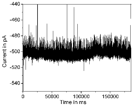
Figure 1: Timeseries of ion-channel currents in open state of Voltage-dependent Anion Channels (VDAC). Four parts have been patched here for extending the data range.

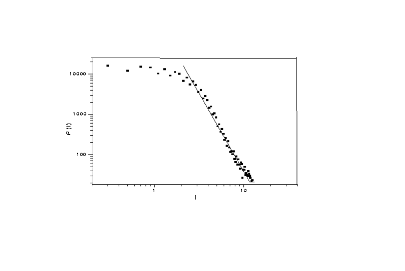
Figure 2: Plot of the probability distribution of magnitudes of current fluctuation $P(I)$ in ion-channel. The best fit is a powerlaw with slope $\alpha=3.86\pm 0.08$.

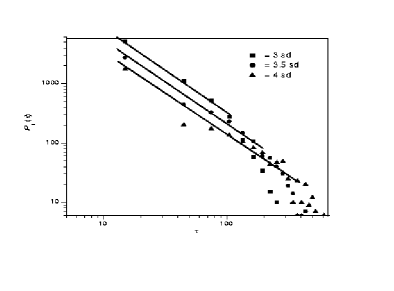
Figure 3: Plot of the probability distribution of recurrence time $P(I_{c},\tau)$for three different threshold currents $I_{c}=3\sigma,3.5\sigma,4\sigma$, where $\sigma$ is the standard deviations. The best fit for all the three plots is a powerlaw with the exponent $\beta=1.47\pm 0.05$.

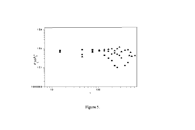
Figure 4: Plot of $P(I_{c},\tau)\tau^{\beta}$ vs. $\tau$.

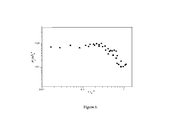
Figure 5: Plot of $P(I_{c},\tau)\tau^{\beta}I_{c}^{\alpha}$ vs. $\tau I_{c}^{-\alpha}$. The resulting plot is the universal function $f(x)$.