Direct observation of a “devil’s staircase” in wave-particle interaction

Abstract

We report the experimental observation of a “devil’s staircase” in a time dependent system considered as a paradigm for the transition to large scale chaos in the universality class of hamiltonian systems. A test electron beam is used to observe its non-self-consistent interaction with externally excited wave(s) in a Travelling Wave Tube (TWT). A trochoidal energy analyzer records the beam energy distribution at the output of the interaction line. An arbitrary waveform generator is used to launch a prescribed spectrum of waves along the slow wave structure (a 4 m long helix) of the TWT. The resonant velocity domain associated to a single wave is observed, as well as the transition to large scale chaos when the resonant domains of two waves and their secondary resonances overlap. This transition exhibits a “devil’s staircase” behavior for increasing excitation amplitude, due to the nonlinear forcing by the second wave on the pendulum-like motion of a charged particle in one electrostatic wave.

Numerous nonlinear driven systems in physics, astronomy, and engineering exhibit striking responses with complex phase-locking plateaus characterized by devil’s staircases. Whereas this structure has fascinated theoreticians since its discovery, and was observed in various condensed matter systems, no dynamical system had so far allowed its direct observation. We realized such an observation for the motion of a charged particle in the potential of two waves. This system has already been used as a theoretical and experimental paradigm for analysing the transition to large scale chaos in conservative systems. Our method consists in measuring the velocity distribution function of a test beam at the outlet of a harmonically excited travelling wave tube. A devil’s staircase is directly measured by varying the amplitude of the excitation in perfect agreement with numerical simulations. This clear experimental realization for a theoretical paradigm opens the possibility to achieve the detailed exploration of chaotic behaviour in non-dissipative systems.

I Introduction

Wave-particle interaction is central to the operation of electron devices and to the understanding of basic plasma behavior and more generally of systems with long range interaction or global coupling. Specifically, travelling wave tubes are ideal to study wave-particle interaction Dim ; Tsu ; APS05 . In the experiments reported here, the electron beam density is so low that it does not induce any significant growth of the waves. When waves are launched in the tube with an external antenna, the beam electrons can be considered as test particles in the potential of electrostatic waves. This recently allowed the direct exploration of nonlinear particle synchronization DovEsc by a single non resonant wave with a phase velocity different from the beam velocity.

In this paper we focus on the resonant case when the beam and the waves propagate with similar velocities. For a single wave, we observe beam trapping in the potential troughs of the wave. When at least two waves propagate we observe a large velocity spread of the essentially mono-kinetic initial beam. This spread can be related to a transition to large scale chaos through resonance overlap and destruction of invariant KAM (Kolmogorov-Arnold-Moser) tori DovAu . We also observe that the velocity spreading is not smooth and occurs through successive steps as the waves amplitudes increase.

The motion of a charged particle in two electrostatic waves has been used as a paradigm system to describe the transition to large-scale chaos in Hamiltonian dynamics Chi ; Esc ; Cha ; Ko ; ElsEsc . It is well known that Hamiltonian phase space exhibits a scale invariance with infinitely nested resonant islands DovEsca . We show that the observed steps in the measured velocity distribution function are related to the underlying “devil’s staircase” behavior.

Numerous nonlinear driven systems in physics, astronomy, and engineering exhibit striking responses with complex phase-locking plateaus characterized by devil’s staircase, Arnold tongues, and Farey trees Lic ; Kad ; Sch ; Ott . These structures are mainly seen at work in stationary and space-extended objects, when an elastic lattice interacts with a periodic substrate found in a wide variety of condensed matter systems including charge-density waves Gor , Josephson junction arrays Ori , Frenkel-Kontorova-type models of friction Flo , unusual growth mode of crystals Hup , and in semiconductor-metal phase transition Ade . They are also at work in the quantum Hall effects Das . But very few dynamical systems have so far allowed their observation. Only indirect observations of statistically locked-in transport through periodic potential landscapes have been made Gop . Here we present a direct experimental evidence of a “devil’s staircase” for wave-particle interaction Mac .

The paper is structured as follows: In Sec. II we present the principle of the test beam experiment in the TWT. In Sec. III, we report the main results on the interaction of the test beam with one or two waves. In Sec. IV, we briefly recall the main results on the transition to large scale chaos in Hamiltonian systems and show some numerical results for the paradigm motion of a charged particle in two waves. In Sec. V, we compare the experimental results with the numerical predictions. Conclusions and perspectives are drawn in Sec. VI.

II Description of the TWT

A travelling wave tube Pie ; Gil consists of two main elements: an electron gun, and a slow wave structure along which waves propagate with a phase velocity much lower than the velocity of light, which may be approximately equal to the electron beam velocity.

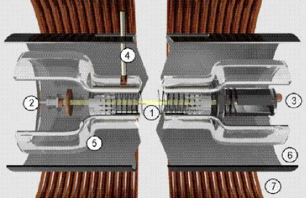
Figure 1: Travelling Wave Tube rendering: (1) helix, (2) electron gun, (3) trochoidal analyzer, (4) antenna, (5) glass vacuum tube, (6) slotted rf ground cylinder, (7) magnetic coil.

The long travelling wave tube sketched in Fig. 1 has been designed to mimic beam-plasma interaction Dim ; Tsu ; APS05 . Its slow wave structure is formed by a helix with axially movable antennas. The electron gun produces a quasi-mono-kinetic electron beam which propagates along the axis of the slow wave structure and is confined by a strong axial magnetic field of $0.05$ T. Its central part consists of the grid-cathode subassembly of a ceramic microwave triode and the anode is replaced by a copper plate with an on-axis hole whose aperture defines the beam diameter equal to $1{\,\rm mm}$. Beam currents, $I_{\mathrm{b}}<1{\,\rm{\mu A}}$, and maximal cathode voltages, $|V_{\mathrm{c}}|<200{\,\rm V}$, can be set independently. Two correction coils (not shown in Fig. 1) provide perpendicular magnetic fields to control the tilt of the electron beam with respect to the axis of the helix.

The slow wave structure consists of a wire helix that is rigidly held together by three threaded alumina rods and is enclosed by a glass vacuum tube. The pump pressure at the ion pumps on both ends of the device is $2\times 10^{-9}{\,\rm Torr}$. The $4{\,\rm m}$ long helix is made of a $0.3{\,\rm mm}$ diameter Be-Cu wire; its radius is equal to $11.3{\,\rm mm}$ and its pitch to $0.8{\,\rm mm}$. A resistive rf termination at each end of the helix reduces reflections. The maximal voltage standing wave ratio is $1.2$ due to residual end reflections and irregularities of the helix. The glass vacuum jacket is enclosed by an axially slotted $57.5{\,\rm mm}$ radius cylinder that defines the rf ground. Inside this cylinder but outside the vacuum jacket are four axially movable antennas labelled from ${\sharp\,1}$ to ${\sharp\,4}$ and azimuthally separated by $90\,^{0}$; they are capacitively coupled to the helix, each of them being characterized by its coupling coefficient which gives the ratio of the amplitude of the wave actually excited on the helix to the amplitude of the signal launched on the antenna; these antennas can excite or detect helix modes in the frequency range from 5 to 95  MHz. Only the helix modes are launched, since empty waveguide modes can only propagate above $2{\,\rm GHz}$. These modes have electric field components along the helix axis Dim . Launched electromagnetic waves travel along the helix at the speed of light; their phase velocities, ${v_{{\mathrm{\varphi}}j}}$, along the axis of the helix are smaller by approximately the tangent of the pitch angle, giving $2.8\times 10^{6}{\,\rm m/s}<{v_{{\mathrm{\varphi}}j}}<5.3\times 10^{6}{\,\rm m/s}$. A beam intensity $I_{\mathrm{b}}$ lower than $150$ nA ensures that the electron beam with mean velocity $v_{\mathrm{b}}$ does not induces any significant wave growth over the tube length; since the potential drop over the beam radius $\delta V=I_{\mathrm{b}}/(4\pi\epsilon_{0}v_{\mathrm{b}})$ is negligible, the beam electrons can be considered as test particles.

Finally the cumulative changes of the electron beam distribution are measured with a trochoidal velocity analyzer at the end of the interaction region. A small fraction ($0.5\%$) of the electrons passes through a hole in the center of the front collector, and is slowed down by three retarding electrodes. By operating a selection of electrons through the use of the drift velocity caused by an electric field perpendicular to the magnetic field, the direct measurement of the current collected behind a tiny off-axis hole gives the time averaged beam axial energy distribution Guy . Retarding potential and measured current are computer controlled, allowing an easy acquisition and treatment with an energy resolution lower than $0.5{\,\rm eV}$.

III Test particle experiments

We first checked that, in the absence of any applied external signal on the antenna, the test electron beam propagates without perturbation along the axis of the device.

III.1 Trapping of the test beam in a resonant wave

In the first experiment, we apply an oscillating signal at a frequency of $f=30$ MHz on antenna ${\sharp\,1}$. According to the helix dispersion relation, a travelling wave propagates along the helix with a phase velocity $v_{\varphi}=4.07\times 10^{6}$ m/s. Fig. 2a shows a 2D contour plot (with logarithmically scaled color coding) of the velocity distribution function for a test beam, with intensity $I_{\mathrm{b}}=120$ nA and initial velocity $v_{\mathrm{b}}=v_{\varphi}$, measured at the outlet of the tube after its interaction, over a length of $2.6$ m, with the helix mode. It is the result of linear interpolation of the recorded measurements obtained for different applied signal amplitudes varying from $0{\,\rm mV}$ to $1400{\,\rm mV}$ by steps of $100{\,\rm mV}$. Each velocity distribution function measurement is obtained by scanning the retarding voltage of the trochoidal velocity analyzer with a step of $61$ mV. When the wave amplitude is gradually increased, we observe that the width of the velocity domain in which the test beam electrons are spread increases like the square root of the wave amplitude as expected if the electrons are trapped in the potential troughs of the wave. No attention must be given to the apparent regular discontinuous steps due to bad sampling of the amplitudes and interpolation between successive measurements. From the measured antenna coupling coefficients Malmberg , the helix wave amplitude $\phi$ can be estimated. The resonant or trapping domain in velocity can thus be deduced and is indicated by the continuous lines in Fig. 2a which correspond to $v_{\varphi}\pm 2\sqrt{\eta\phi}$; here $\eta$ is the charge to mass ratio of the electron. We observe a very good agreement with measurement.

Fig. 2b is obtained in the same way as Fig. 2a but corresponds to a larger interaction length since the emitting antenna is located at $L=3.5$ m from the device output. Each velocity distribution function measurement is obtained by scanning the retarding voltage of the trochoidal velocity analyzer with a step of $240$ mV to speed up data acquisition without deteriorating significantly the accuracy of our observations. We observe that the shape of the velocity domain in which the test beam electrons are spread is very different from Fig. 2a. A new feature appearing in Fig. 2b is a further velocity bunching of the electrons around their initial velocity for an amplitude equal to $600{\,\rm mV}$. This phenomenon is also related to the trapping of the electrons in the wave. If we refer to the rotating bar model Myn to describe the trapped electrons motion, we expect oscillations between small spread in velocity and large spread in position (corresponding to initial conditions for a cold test beam) to large spread in velocity and small spread in position after half a bounce or trapping period equal to $T_{b}/2=v_{\varphi}/(2f\sqrt{\eta\phi})$. To the bounce period, we can associate a bounce length $L_{b}=v_{\varphi}T_{b}$. For $\phi=35{\,\rm mV}$, we get $L_{b}/2=350{\,\rm cm}$ which is precisely the interaction length $L$ of Fig. 2b. We thus confirm that Fig. 2 is displaying the trapping of the test beam in a single wave. Varying $I_{\mathrm{b}}$ from $10$ to $150$ nA would not change the result since no self-consistent effect occurs. One may remark that Fig. 2 also displays a systematic accumulation of particles in the high velocity region for which we do not have a simple explanation and which probably requires further investigation out of the scope of the present paper.

III.2 Test beam interacting with two waves

In the second experiment, we apply, on antenna ${\sharp\,2}$ chosen for its strongest coupling with the helix and located at $L=3.5$ m from the device output, a signal generated by an arbitrary waveform generator made of two components with well defined phases: again one at the same frequency of $30$ MHz, and a new one at a frequency of $60$ MHz. According to the helix dispersion relation, two travelling waves propagate along the helix, the former with a phase velocity $v_{\varphi 1}=4.07\cdot 10^{6}$ m/s as before, the latter with a different phase velocity $v_{\varphi 2}=3.08\cdot 10^{6}$ m/s (the fact that the second wave is a harmonic of the first one in the laboratory frame is irrelevant in the beam frame).

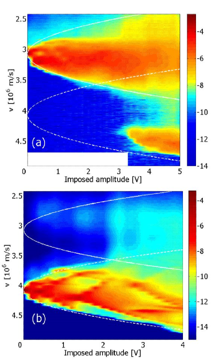
Figure 3: 2D contour plot of the measured velocity distribution function (with logarithmically scaled color coding) of a test beam ($I_{\mathrm{b}}=10{\,\rm nA}$) interacting with two waves at 30 MHz and 60 MHz with trapping domains (continuous and dashed curves) for increasing amplitude and fixed interaction length $L=3.6{\,\rm m}$: a) $v_{\mathrm{b}}=3.55\times 10^{6}{\,\rm{m/s}}$, b) $v_{\mathrm{b}}=4.07\times 10^{6}{\,\rm{m/s}}$ EndNote29 .

Fig. 3a (resp. Fig. 3b) is obtained in the same way as Fig. 2 for a test beam, with intensity $I_{\mathrm{b}}=10$ nA and initial velocity $v_{\mathrm{b}}=v_{\varphi 1}$ (resp. $v_{\mathrm{b}}=v_{\varphi 2}$), whose velocity distribution function is measured at the outlet of the tube after its interaction with the two propagating helix modes. As in Fig. 2 the continuous (resp. dashed) parabola shows the trapping velocity domain associated to the helix mode at $60$ MHz (resp. $30$ MHz). As it appears clearly, the amplitudes of the two modes have been appropriately chosen such that these trapping domains approximately have the same velocity extension when taking into account the coupling coefficient of the antenna at the two working frequencies. Both in Fig. 3a and Fig. 3b, we observe that, for a threshold amplitude exceeding the amplitude corresponding to overlap of the trapping domains, the velocity distribution function exhibits a strong velocity spread. Electrons initially trapped inside the potential well of one of the helix modes can escape the trapping domain and explore a much wider velocity region in phase space. According to their initial velocity, electrons can be strongly accelerated (Fig. 3a) or decelerated (Fig. 3b) sticking mainly to the border of the new velocity domain they are allowed to explore. We shall later relate this behavior to the transition to large scale chaos for the motion of a charged particle in two electrostatic waves. Such a description would suggest that Fig. 3b could be obtained by a mere reflection of Fig. 3a with respect to the average velocity of the two waves. The observed asymmetry can result from the different transit times of the test particles over the finite length of the tube in both cases, and from the already noticed accumulation of particles toward higher velocities of Fig. 2.

III.3 Test beam and excitation at a single frequency

In the third experiment, we apply an oscillating signal at a frequency of $30$ MHz on antenna ${\sharp\,2}$ as in the first experiment for maximum interaction length $L=3.5$ m. But we now consider a test beam, with intensity $I_{\mathrm{b}}=10$ nA and initial velocity $v_{\mathrm{b}}=2.7\cdot 10^{6}$ m/s much lower than $v_{\varphi}$, the phase velocity of the helix mode at $30$ MHz. Fig. 4 is obtained in the same way as Fig. 2. The continuous parabola indicates the velocity domain associated to particle trapping in the potential troughs of the helix mode at $30$ MHz. Since the initial beam velocity lies far out of this domain we expect that, for moderate wave amplitude, the beam electrons will experience a mere velocity modulation around their initial velocity, with a modulation amplitude increasing linearly with the applied signal amplitude. This behavior has been studied in detail in Ref. [3] and would generate two main peaks around the (oblique straight) continuous lines originating in $v_{\mathrm{b}}$.

In fact we observe that the electrons spread over a velocity domain with typical width increasing as the square root of the applied signal amplitude as shown by the dashed parabola. This strongly recalls the results of Fig. 2. Indeed the applied signal generates two waves: a helix mode with a phase velocity $v_{\varphi}$, and a beam mode with a phase velocity equal to the beam velocity $v_{\mathrm{b}}$. The beam mode with phase velocity $v_{\mathrm{b}}$ is actually the superposition of two indistinguishable modes with pulsation $\omega=kv_{\mathrm{b}}\pm\omega_{\mathrm{b}}$ corresponding to the beam plasma mode with pulsation $\omega_{\mathrm{b}}=[n_{\mathrm{b}}e^{2}/(m\epsilon_{0})]^{1/2}$ for a beam with density $n_{\mathrm{b}}$, Doppler-shifted by the beam velocity $v_{\mathrm{b}}$, merging in a single mode since $\omega_{\mathrm{b}}\ll\omega$ in our conditions Pie . Thus Fig. 4 shows the test electrons trapping into the beam mode. This is confirmed by a careful analysis of Fig. 4 which exhibits the same velocity bunching of the electrons around their initial velocity as in Fig. 2a, for amplitudes obtained by equating the interaction length to a multiple of half the trapping length. One also notices that the amplitude of the beam mode is lower than the amplitude of the launched helix mode; this explains why its influence has been neglected in the previous analysis of Fig. 3 where two helix modes are externally excited. Since, when we increase the applied signal amplitude in Fig. 4, the two trapping domains of the helix and the beam mode overlap, we observe the same behavior as in Fig. 3. Above a certain applied signal amplitude threshold the distribution function spreads over a much wider velocity domain, and electrons can be strongly accelerated.

Another striking feature appears in Fig. 4, which is best emphasized in the zoom of Fig. 5a. The transition to large velocity spread does not occur continuously but rather occurs by steps when the applied signal amplitude increases. As shown in Fig. 5b, plateaus are formed in the measured velocity distribution function for the maximum interaction length. A closer look at Fig. 3 also reveals the presence of such steps in the case of two independently launched waves with equal amplitudes. We will now show that this generic phenomenon is related to the intrinsic structure of Hamiltonian phase space for non integrable systems.

IV Motion of a test charged particle and Hamiltonian chaos

We consider charged test particles moving in two electrostatic waves. The equation modelling the dynamics in this case is

$$\ddot{x}=\sum_{{\it i}=1}^{2}\eta k_{i}\phi_{i}\sin(k_{i}x-\omega_{i}t+\varphi_{i}).$$ (1)

where $\phi_{i}$, $k_{i}$, $\omega_{i}$ and $\varphi_{i}$ are respectively the amplitudes, wave numbers, frequencies and phases of the two waves; $\eta$ is the charge to mass ratio of the particle.

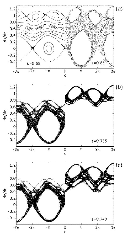
Figure 6: Poincaré surface of section for the dynamics given by $\ddot{x}=-\varepsilon(\sin(x)+0.16k\sin k(x-t))$, with $k=5/3$, for which $s=2.8\sqrt{\varepsilon}$. (a) Left half for $\varepsilon\simeq 0.39~{}(s=0.55)$ exhibits island chains of secondary resonances at rational velocities $m/(n+m)$, as seen from 15 orbits which do not mix ; right half for $\varepsilon\simeq 0.92~{}(s=0.85)$ exhibits large scale chaos as seen for two orbits. (b) Two orbits related to upper and lower main chaotic domains for $s=0.735$, each iterated over $10^{5}$ Poincaré periods  ; to allow an easy comparison, only points with $-3\pi<(x~{}{\mathrm{mod}}~{}6\pi)<0$ are plotted for one orbit, and $0<(x~{}{\mathrm{mod}}~{}6\pi)<3\pi$ for the other orbit. (c) Similar plot for $s=0.74$.

The motion of the particles governed by this equation is a mixture of regular and chaotic behaviors mainly depending on the amplitudes of the waves Chi ; Esc ; ElsEsc and exhibits generic features of chaotic systems Lic ; Kad ; Sch ; Ott . Poincaré sections of the dynamics (a stroboscopic plot of selected trajectories) are displayed in Fig. 6. Taking advantage of the symmetry $x^{\prime}=-x$, two different cases are superposed in Fig. 6. The strength of chaos is measured by the dimensionless overlap parameter defined as the ratio

$$s=\frac{2(\sqrt{\eta\phi_{1}}+\sqrt{\eta\phi_{2}})}{|v_{\varphi 1}-v_{\varphi 2}|}$$ (2)

of the sum of the resonant velocity half-widths of the two wave potential wells to their phase velocity difference Chi .

For intermediate wave amplitudes, nested regular structures appear as secondary resonances with a wave number $k_{nm}=nk_{1}+mk_{2}$, a frequency $\omega_{nm}=n\omega_{1}+m\omega_{2}$, a phase $\varphi_{nm}=n\varphi_{1}+m\varphi_{2}$ and an effective amplitude $\phi_{nm}\sim\phi_{1}^{|n|}\phi_{2}^{|m|}$ with integer $n$ and $m$, as shown in the left side of Fig. 6a for $s=0.55$. The self-similar structure of phase space results from the infinitely nested higher order resonances DovEsca which appear in so-called Arnold tongues between secondary resonances as predicted by the Poincaré-Birkhoff theorem Arn .

For larger wave amplitudes, a wide connected zone of chaotic behavior occurs in between the primary resonances due to the destruction of the so-called Kolmogorov-Arnold-Moser (KAM) tori acting as barriers in phase space, as shown in the right side of Fig. 6a for $s=0.85$. Between these two values of $s$, invariant tori are sequentially destroyed and replaced by cantori. Transport in velocity (and thereby in $(x,v)$ space) occurs through the holes of the cantori, which have a fractal structure Meiss . When a torus breaks, the flux through it is still zero, as the associated turnstile has vanishing area : trajectories leak easily through its holes only for $s$ values significantly above its destruction threshold. For the dynamics $\ddot{x}=-\varepsilon(\sin(x)+0.16k\sin k(x-t))$, with $k=5/3$, which is close to our experimental conditions, the threshold for large scale chaos (destruction of the most robust torus) is near $s\approx 0.75$, as seen from the Poincaré section of orbits over long times (Fig.6, (b-c)).

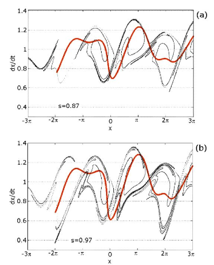
Figure 7: Evolution of the beam initially at $v=1$ for the same dynamics as Fig. 6, for values of $s$ around the most prominent step at times $\tau=6\pi/5$ (bold, red dots) and $\tau=12\pi$ (small, black dots).

If one considers a beam of initially monokinetic particles having a velocity equal to the phase velocity of one of the waves, this chaotic zone is associated with a large spread of the velocities after some time since the particles are moving in the chaotic sea created by the overlap of the two resonances Esc ; ElsEsc . In analogy with the experimental conditions, we compute (with a second order centered symplectic integrator) the trajectories of 1 million particles initially uniformly spread in position with the same velocity (equal to 1). As seen in fig. 7, as the overlap parameter increases, the beam wiggles more and is spread over a wider velocity range EndNote30a .

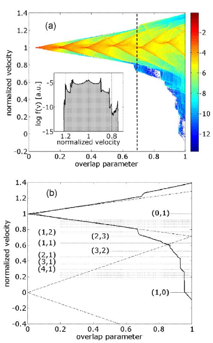
Figure 8: Numerical devil’s staircase. a) Probability distribution function $f(v)$ (with logarithmically scaled color coding) of the velocity for the dynamics of Fig. 6, as a function of overlap parameter $s=2.8\sqrt{\varepsilon}$ after a time $\tau=12\pi$, i.e. $10$ Poincaré stroboscopic periods (inset, $f(v)$ for the value of $s$ indicated by the vertical dashed line). b) Velocity frontiers of $f(v)$ versus $s$ for $t=12\pi$; dashed oblique lines starting from $v=0$ and $v=1$ indicate the primary resonances trapping domains; secondary resonances $(n,m)$ are indicated at rational velocities $mk/(n+mk)$.

As shown in Figs. 8 and $9$, the transition to large scale chaos occurs by vertical steps, related to the presence of the nested secondary resonances, with height scaling as the amplitudes $\phi_{nm}$. Therefore the border of the velocity domain over which the beam is spread exhibits a devil’s staircase-like behavior. Fig. 8a is the result of applying the same treatment as applied to experimental data in section III to the computed velocity distribution function obtained for different overlap parameters varying from 0 to 1 by steps of $0.01$ keeping the wave amplitude ratio constant and approximately equal to the experimental value of Fig. 4. Each velocity distribution function is obtained by recording the velocity histogram of our $10^{6}$ particles over 1600 boxes with normalized velocity width equal to $0.001$ after an integration time $\tau$ equal to 10 Poincaré periods. Even for an overlap parameter equal to 1, during the integration time $\tau$, the particles could not explore the whole chaotic sea between the two main resonances. But the particles could typically experience one complete trapping motion as shown by the periodic velocity bunching and related same horizontally wedge-shaped regions as experimentally observed in Fig. 2. An asymmetric plateau EndNote30b is formed in the velocity distribution function as exemplified in the insert of Fig. 8a. The detailed analysis of the border of the distribution function displayed in Fig. 8b shows that this plateau can be associated to the secondary resonance characterized by integers $m=n=1$.

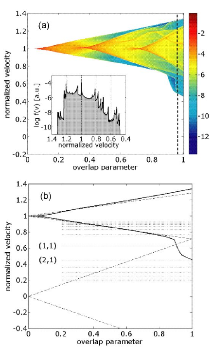
Figure 9: Numerical devil’s staircase after a time $\tau=24\pi$, i.e. $20$ Poincaré stroboscopic periods. a) Probability distribution function $f(v)$. b) Velocity frontiers of $f(v)$.

Fig. 9 is obtained in the same way as Fig. 8 but corresponds to a longer integration time $\tau$ equal to 20 Poincaré periods. Now the particles can explore the whole chaotic sea in between the two main resonances, and finer details of the “devil’s staircase” associated to the presence of the nested secondary resonances can be observed. In Fig. 9b showing the low velocity border of the computed chaotic domain, the position of some of the most important secondary resonances is indicated with a label corresponding to their characteristic integers $(n,m)$. It appears clearly that the presence of a secondary resonance results in a step in the 2D contour plot of the distribution function. The most striking feature is the great similarity with the above experimental results which can now be reexamined in the light of the two-waves model.

V Discussion

To allow easier comparison with numerical simulations, we compute the overlap parameter of the helix and the beam modes. The wave amplitude can be estimated by fitting the trapping domain with a parabola as shown in Fig. 2 to Fig. 4. As already mentioned, we checked that, for the helix mode, this estimate is in very good agreement with the amplitude deduced from measuring the antenna coupling coefficient with three antennas Malmberg . Then we display the upper velocity domain border (i.e. the location of the upper steep edge of the plateau as shown in Fig. 5b) as the applied signal amplitude is varied. We thus obtain Fig. 5c. The experimentally observed steps are clearly related to the presence of secondary resonances labelled $(1,m)$ with $m$ = 1, 2, 3.

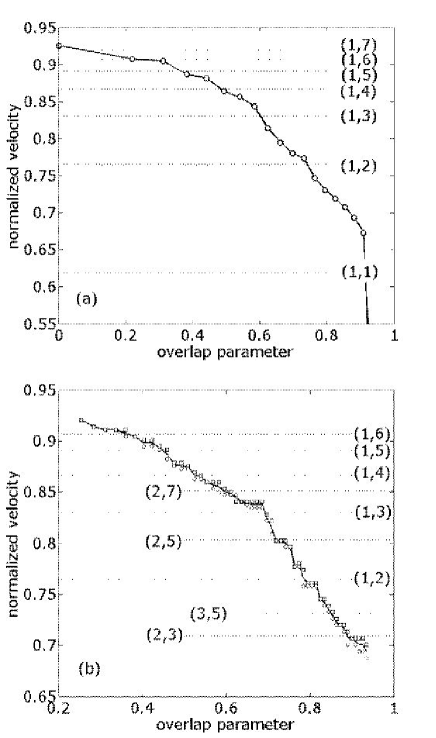
Figure 10: Experimental devil’s staircase: plot versus overlap parameter of the upper normalized velocity frontier of $f(v)$ for a test beam ($I_{\mathrm{b}}=10{\,\rm nA},v_{\mathrm{b}}=2.5\times 10^{6}{\,\rm{m/s}}$) with applied signal at 30 MHz for increasing amplitude and fixed interaction length $L=3.6{\,\rm m}$ with (a) coarse and (b) fine signal amplitude scan; velocity normalization is such that $v=0$ (resp. 1) stands for the helix (resp. beam) mode phase velocity; secondary resonances $(n,m)$ are indicated at velocities $m\kappa/(n+m\kappa)$ with $\kappa=v_{\mathrm{\varphi}}/v_{\mathrm{b}}$.

For a different initial beam velocity, Fig. 10a shows the upper velocity domain border as the applied signal amplitude is varied by steps of $1.5$ V; only the steps associated to the main secondary resonances $(1,n)$ for $n=1...6$ can be observed. The points plotted are the outcome of a single set of measurements; the solid line is a guide to the eye. By reducing the signal amplitude steps to $0.5$ V, more details of the devil’s staircase can be observed and higher order resonances show up. For example, in Fig. 10b, more steps are observed such as $(2,3)=(1,1)+(1,2)$, $(2,5)$ and $(2,7)$ which stand among the next strongest resonances in the Farey tree structure. In this latter plot, two new, independent measurements have been reported (as circles and squares) EndNote30c to give an estimate of the experimental errors, and the solid line interpolates between their averages. The behavior reported in Fig. 10a and Fig. 10b is typical of self-similar phenomena.

It is worth mentioning that we focused our attention on the velocity domain in between the two main resonances. As shown by the upper part of Fig. 4a, we also observe vertical steps associated with resonances (1,-5) and (1,-6); this feature is also obvious in the numerical simulation of Fig. 9 where a step associated with resonance (1,-3) clearly appears on the upper part. Since numerical simulations deal with a restricted number of particles (typically 1 million), only the steps associated with lower $m$’s appear.

VI Conclusion and perspectives

We have thus exhibited that measuring the energy distribution of the electron beam at the output of a travelling wave tube allows a direct experimental exploration of fractal features of the complex Hamiltonian phase space. It constitutes a direct experimental evidence of a “devil’s staircase” in a time-dependent system.

This knowledge opens new tracks in the study of these systems:

-It allowed accurate experiments aimed at investigating Hamiltonian phase space APS05 and testing new methods of control of Hamiltonian chaos Chan .

-It is a step in the direction of experimental assessment of the still open question of quasilinear diffusion in a broad spectrum of waves Car excited with the arbitrary waveform generator DovGuy .

-Time resolved measurements of the evolution of electron bunches injected with a prescribed phase with respect to a wave Bou should allow to explore more details about the test particle dynamics.

-The influence of self-consistent effects could be studied by gradually increasing the beam intensity.

Beside their fundamental importance, these studies can find direct useful applications in the fields of :

-plasma physics,

-control of complex systems,

-electron devices such as travelling wave tubes and free electron lasers where improvement of performances are of crucial importance.

The authors are grateful to J-C. Chezeaux, D. Guyomarc’h, and B. Squizzaro for their skillful technical assistance, and to C. Chandre and D.F. Escande for fruitful discussions. This work is supported by Euratom/CEA. A. Macor benefits from a grant by Ministère de la Recherche. Y. Elskens benefited from a delegation position with Centre National de la Recherche Scientifique.

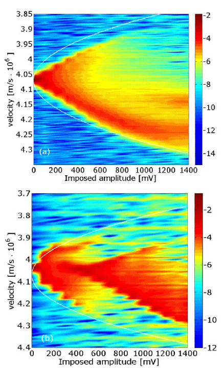
Figure 2: 2D contour plot of the measured velocity distribution function (with logarithmically scaled color coding) of a test beam ($I_{\mathrm{b}}=120{\,\rm nA},v_{\mathrm{b}}=4.07\times 10^{6}{\,\rm{m/s}}$) trapped in a single wave at 30 MHz with trapping domain (continuous curve) for increasing amplitude and fixed interaction length: a) $L=2.6{\,\rm m}$, b) $L=3.5{\,\rm m}$.

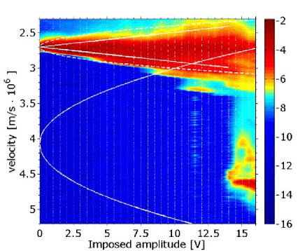
Figure 4: 2D contour plot of the measured velocity distribution function (with logarithmically scaled color coding) of a test beam ($I_{\mathrm{b}}=10{\,\rm nA},v_{\mathrm{b}}=2.7\times 10^{6}{\,\rm{m/s}}$) with applied signal at 30 MHz for increasing amplitude and fixed interaction length $L=3.6{\,\rm m}$ (trapping domains of helix and beam modes are indicated by continuous and dashed parabolas).

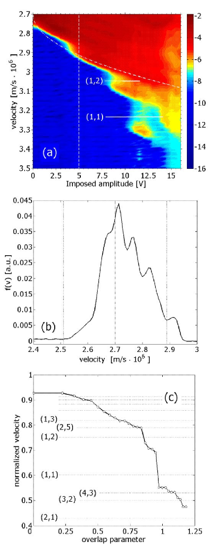
Figure 5: a) Zoom of Fig. 4. b) Beam velocity distribution function for amplitude corresponding to the dashed vertical line in the above figure. c) Normalized upper velocity frontier of $f(v)$ versus overlap parameter $s$; velocity normalization is such that $v=0$ (resp. 1) stands for the helix (resp. beam) mode phase velocity; secondary resonances $(n,m)$ are indicated at velocities $m\kappa/(n+m\kappa)$ with $\kappa=v_{\mathrm{\varphi}}/v_{\mathrm{b}}$.

References

- (1) G. Dimonte and J.H. Malmberg, Phys. Fluids 21, 1188 (1978).
- (2) S.I. Tsunoda, F. Doveil and J.H. Malmberg, Phys. Rev. Lett. 58, 1112 (1987).
- (3) F. Doveil and A. Macor, Phys. Plasmas 13, in press (2006).
- (4) F. Doveil, D.F. Escande and A. Macor, Phys. Rev. Lett. 94, 085003 (2005).
- (5) F. Doveil, Kh. Auhmani, A. Macor and D. Guyomarc’h, Phys. Plasmas 12, 010702 (2005).
- (6) B.V. Chirikov, Phys. Rep. 52, 263 (1979).
- (7) D.F. Escande, Phys. Rep. 1212, 165 (1985).
- (8) C. Chandre and H.R. Jauslin, Phys. Rep. 365, 1 (2002).
- (9) H. Koch, Disc. Cont. Dyn. Syst. 11, 881 (2004).
- (10) Y. Elskens and D.F. Escande, Microscopic dynamics of plasmas and chaos (IoP Publishing, Bristol, 2003).
- (11) F. Doveil and D.F. Escande, Phys. Lett. 90A, 226 (1982).
- (12) A.J. Lichtenberg and M.A. Lieberman, Regular and chaotic dynamics (Springer, New York, 1992).
- (13) L.P. Kadanoff, From order to chaos: Essay: Critical, chaotic and otherwise (World Scientific, Singapore, 1993); II (1998).
- (14) H.G. Schuster, Deterministic chaos (VCH Verlag, Weinheim, 1988).
- (15) E. Ott, Chaos in dynamical system (Cambridge university press, Cambridge, 1993).
- (16) L.P. Gor’kov and G. Grüner, Charge density waves in solids (Elsevier, Amsterdam, 1989).
- (17) S.E. Hebboul and J.C. Garland, Phys. Rev B 47, 5190 (1993); E. Orignac and T. Giamarchi, Phys. Rev. B 64, 144515 (2001).
- (18) L. Floria and F. Falo, Phys. Rev. Lett. 68, 2713 (1992); O.M. Braun, A.R. Bishop, and J. Röder, Phys. Rev. Lett. 79, 3692 (1997).
- (19) P. Pieranski, P. Sotta, D. Rohe, and M. Imperor-Clerc, Phys. Rev. Lett. 84, 2409 (2000); M. Hupalo, J. Schmalian and M.C. Tringides, Phys. Rev. Lett. 90, 216106 (2003).
- (20) D. Adelman, C.P. Burmester, L.T. Wille, P.A. Sterne and R. Gronsky, J. Phys.: Cond. Matter 4, L585 (1992).
- (21) S. Das Sarma and A. Pinczuk, Perspective in quantum Hall effects (Wiley, New York, 1997).
- (22) A. Gopinathan and D.G. Grier, Phys. Rev. Lett. 92, 130602 (2004).
- (23) A. Macor, F. Doveil, and Y. Elskens, Phys. Rev. Lett. 95, 264102 (2005).
- (24) J.R. Pierce, Traveling wave tubes (Van Nostrand, New York, 1950).
- (25) A.S. Gilmour Jr, Principles of traveling wave tube (Artech House, London, 1994).
- (26) D. Guyomarc’h and F. Doveil, Rev. Sci. Instrum. 71, 4087 (2000).
- (27) J.H. Malmberg, T.H. Jensen and T.M. O’Neil, Plasma Phys. Controlled Nucl. Fusion Res. 1, 683 (1966)
- (28) H.E. Mynick and A.N. Kaufman, Phys. Fluids 21, 653 (1978).
- (29) Two causes can contribute to the presence of slower electrons: i) the gun itself, ii) space charge effects in the trochoidal analyzer. The normalization of the velocity distribution function enhances this lower tail when the beam is more spread (hence the observed periodicity at low wave amplitude, low electron velocity in Fig. 3b). Fig. 3a which focuses on accelerated electrons is not polluted by these low energy electrons in the relevant domain.
- (30) V.I. Arnold, Mathematical methods of classical mechanics (Nauka, Moscow, 1974).
- (31) J.D. Meiss, Rev. Mod. Phys. 64, 795 (1992).
- (32) As the beam intersects the core of the cat eye, part of it merely rotates in the trapping domain. One should not mistake the image of the beam at later times, as in Fig. 7, with the unstable manifold of the hyperbolic point associated with the wave. However, the wiggles of the beam in the chaotic domain must follow grossly the wiggles of this unstable manifold.
- (33) The many small peaks in the plot of are the result of the foldings of the smooth curve in space which was initially the monokinetic beam at . The probability density in diverges at each fold like the classical arc sine law.
- (34) The squares are above the circles because they correspond to a lower estimate of the noise level.
- (35) C. Chandre, G. Ciraolo, F. Doveil, R. Lima, A. Macor and M. Vittot, Phys. Rev. Lett 94, 074101 (2005).
- (36) J.R. Cary, D.F. Escande, and A.D. Verga, Phys. Rev. Lett. 65, 3132 (1990).
- (37) F. Doveil and D. Guyomarc’h, Comm. Nonlinear Sci. Numerical Simulation 8, 529 (2003).
- (38) A. Bouchoule and M. Weinfeld, Phys. Rev. Lett. 36, 1144 (1976).