Compressible advection of a passive scalar: Two-loop scaling regimes

Abstract

The influence of compressibility on the stability of the scaling regimes of the passive scalar advected by a Gaussian velocity field with finite correlation time is investigated by the field theoretic renormalization group within two-loop approximation. The influence of compressibility on the scaling regimes is discussed as a function of the exponents $\varepsilon$ and $\eta$, where $\varepsilon$ characterizes the energy spectrum of the velocity field in the inertial range $E\propto k^{1-2\varepsilon}$, and $\eta$ is related to the correlation time at the wave number $k$ which is scaled as $k^{-2+\eta}$. The restrictions given by nonzero compressibility on the regions with stable infrared fixed points which correspond to the stable infrared scaling regimes are discussed in detail. A special attention is paid to the case of so-called frozen velocity field, when the velocity correlator is time independent. In this case, explicit inequalities which must be fulfilled in the plane $\varepsilon-\eta$ are determined within two-loop approximation. The existence of a ”critical” value $\alpha_{c}$ of the parameter of compressibility $\alpha$ at which one of the two-loop conditions is canceled as a result of the competition between compressible and incompressible terms is discussed. Brief general analysis of the stability of the scaling regime of the model with finite correlations in time of the velocity field within two-loop approximation is also given.

, , ,

1 Introduction

One of the main problems in the modern theory of fully developed turbulence is to verify the validity of the basic principles of Kolmogorov-Obukhov (KO) phenomenological theory and their consequences within the framework of a microscopic model [1, 2]. On the other hand, recent experimental, numerical and theoretical studies signify the existence of deviations from the well-known Kolmogorov scaling behavior. The scaling behavior of the velocity fluctuations with exponents, which values are different from Kolmogorov ones, is known as anomalous and is associated with intermittency phenomenon [2]. Even thought the understanding of the intermittency and anomalous scaling within the theoretical description of the fluid turbulence on basis of the ”first principles”, i.e., on the stochastic Navier-Stokes equation, still remains an open problem, considerable progress has been achieved in the studies of the simplified model systems which share some important properties of the real turbulence.

The crucial role in these studies is played by models of advected passive scalar field [3]. Maybe the most known model of this type is a simple model of a passive scalar quantity advected by a random Gaussian velocity field, white in time and self-similar in space, the so-called Kraichnan’s rapid-change model [4]. It was shown by both natural and numerical experimental investigations that the deviations from the predictions of the classical KO phenomenological theory is even more strongly displayed for a passively advected scalar field than for the velocity field itself (see, e.g., [5] and references cited therein). At the same time, the problem of passive advection is much more easier to be consider from theoretical point of view. There, for the first time, the anomalous scaling was established on the basis of a microscopic model [6], and corresponding anomalous exponents was calculated within controlled approximations (see review [5] and references therein).

In paper [7] the field theoretic renormalization group (RG) and operator-product expansion (OPE) were used in the systematic investigation of the rapid-change model. It was shown that within the field theoretic approach the anomalous scaling is related to the very existence of so-called ”dangerous” composite operators with negative critical dimensions in OPE (see, e.g., [8, 9] for details). Important advantages of the RG approach are its universality and calculational efficiency: a regular systematic perturbation expansion for the anomalous exponents was constructed, similar to the well-known $\epsilon$-expansion in the theory of phase transitions.

Afterwards, various generalized descendants of the Kraichnan model, namely, models with inclusion of large and small scale anisotropy [10], compressibility [11] and finite correlation time of the velocity field [12, 13] were studied by the field theoretic approach. General conclusion is: the anomalous scaling, which is the most important feature of the Kraichnan rapid change model, remains valid for all generalized models.

In paper [12] the problem of a passive scalar advected by the Gaussian self-similar velocity field with finite correlation time [15] was studied by the field theoretic RG method. There, the systematic study of the possible scaling regimes and anomalous behavior was present at one-loop level. The two-loop corrections to the anomalous exponents were obtained in [18]. In paper [13] the influence of compressibility on the problem studied in [12] was analyzed. In what follows, we shall continue with the investigation of this model from the point of view of the influence of compressibility on the stability of the scaling regimes within two-loop approximation. It can lead to sufficient restrictions of the parameter space where the stable fixed points can exist. This, as we shall see rather complicated task, is the first nontrivial step on the way to understand the influence of the compressibility of the system on the two-loop corrections to anomalous dimensions of the measurable quantities [18].

2 Description of the model

We consider the advection of a passive scalar field $\theta\equiv\theta(x)\equiv\theta(t,{\bf x})$ which is described by the stochastic equation

$$\partial_{t}\theta+v_{i}\partial_{i}\theta=\nu_{0}\Delta\theta+f^{\theta},$$ (1)

where $\partial_{t}\equiv\partial/\partial t$, $\partial_{i}\equiv\partial/\partial x_{i}$, $\nu_{0}$ is the coefficient of molecular diffusivity (hereafter all parameters with a subscript $0$ denote bare parameters of unrenormalized theory; see below), $\Delta\equiv\partial^{2}$ is the Laplace operator, and $f^{\theta}\equiv f^{\theta}(x)$ is a Gaussian random noise with zero mean and correlation function

$$\langle f^{\theta}(x)f^{\theta}(x^{\prime})\rangle=\delta(t-t^{\prime})C({\bf r}/L),\,\,\,{\bf r}={\bf x}-{\bf x^{\prime}},$$ (2)

where parentheses $\langle...\rangle$ hereafter denote average over corresponding statistical ensemble. The noise maintains the steady-state of the system but the concrete form of the correlator is not essential. The only condition which must be fulfilled by the function $C({\bf r}/L)$ is that it must decrease rapidly for $r\equiv|{\bf r}|\gg L$, where $L$ denotes an integral scale related to the stirring. The velocity field ${\bf v(x)}$ obeys a Gaussian distribution with zero mean and correlator [13]

$$\langle v_{i}(x)v_{j}(x^{\prime})\rangle = D^{v}_{ij}(x,x^{\prime})$$

$$= \int\frac{d\omega d^{d}k}{(2\pi)^{d+1}}\left(P_{ij}({\bf k})+\alpha Q_{ij}({\bf k})\right)\tilde{D}^{v}(\omega,k)\exp[-i\omega(t-t^{\prime})+i{\bf k}({\bf x}-{\bf x^{\prime}})],$$

where $k=|{\bf k}|$ is the wave number, $\omega$ is frequency, $d$ is the dimensionality of the ${\bf x}$ space. In what follows, we shall work with compressible velocity field which is demonstrated by the form of the tensor structure of the correlator (2), namely, it consists of two parts: the standard transverse projector $P_{ij}({\bf k})=\delta_{ij}-k_{i}k_{j}/k^{2}$, and the longitudinal projector $Q_{ij}({\bf k})=k_{i}k_{j}/k^{2}$ which is related to compressibility. The parameter $\alpha\geq 0$ is a free parameter. The value $\alpha=0$ corresponds to the divergence-free (incompressible) advecting velocity field. The function $\tilde{D}^{v}$ is chosen as follows [12, 13]

$$\tilde{D}^{v}(\omega,k)=\frac{g_{0}\nu_{0}^{3}k^{4-d-2\varepsilon-\eta}}{(i\omega+u_{0}\nu_{0}k^{2-\eta})(-i\omega+u_{0}\nu_{0}k^{2-\eta})}.$$ (4)

The correlator (4) is related to the energy spectrum via the frequency integral

$$E(k)\simeq k^{d-1}\int d\omega\tilde{D}^{v}(\omega,k)\simeq\frac{g_{0}\nu_{0}^{2}}{u_{0}}k^{1-2\varepsilon}.$$ (5)

It means that the coupling constant $g_{0}$ (more precisely $g_{0}/u_{0}$ [13]) and the exponent $\varepsilon$ describe the equal-time velocity correlator or, equivalently, energy spectrum. On the other hand, the constant $u_{0}$ and the second exponent $\eta$ are related to the frequency $\omega\simeq u_{0}\nu_{0}k^{2-\eta}$ which characterizes the mode $k$. Thus, in our notation, the value $\varepsilon=4/3$ corresponds to the well-known Kolmogorov ”five-thirds law” for the spatial statistics of velocity field, and $\eta=4/3$ corresponds to the Kolmogorov frequency. Simple dimensional analysis shows that the charges $g_{0}$ and $u_{0}$ are related to the characteristic ultraviolet (UV) momentum scale $\Lambda$ (of the order of inverse Kolmogorov length) by

$$g_{0}\simeq\Lambda^{2\varepsilon+\eta},\,\,\,u_{0}\simeq\Lambda^{\eta}.$$ (6)

In the end of this section, let us briefly discuss two important limits of the considered model (2), (4) (see also [12, 13]). First of them is so-called rapid-change model limit when $u_{0}\rightarrow\infty$ and $g_{0}^{\prime}\equiv g_{0}/u_{0}^{2}=$ const,

$$\tilde{D}^{v}(\omega,k)\rightarrow g_{0}^{\prime}\nu_{0}k^{-d-2\varepsilon+\eta},$$ (7)

and the second one is so-called quenched (time-independent or frozen) velocity field limit which is defined by $u_{0}\rightarrow 0$ and $g_{0}^{\prime\prime}\equiv g_{0}/u_{0}=$ const,

$$\tilde{D}^{v}(\omega,k)\rightarrow g_{0}^{\prime\prime}\nu_{0}^{2}k^{-d+2-2\varepsilon}\pi\delta(\omega).$$ (8)

Here the velocity correlator is independent of time in the $t$ representation.

3 Field Theoretic Formulation of the Model

The stochastic problem (1)-(2) is equivalent to the field theoretic model of the set of fields $\Phi\equiv\{\theta,\theta^{\prime},{\bf v}\}$ (see, e.g., [8, 19]) with action functional

$$S(\Phi)= - \frac{1}{2}\int dt_{1}\,d^{d}{\bf x_{1}}\,dt_{2}\,d^{d}{\bf x_{2}}\,\,v_{i}(t_{1},{\bf x_{1}})[D^{v}_{ij}(t_{1},{\bf x_{1}};t_{2},{\bf x_{2}})]^{-1}v_{j}(t_{2},{\bf x_{2}})$$ (9)

$$+ \int dt\,d^{d}{\bf x}\,\,\theta^{\prime}\left[-\partial_{t}\theta-v_{i}\partial_{i}\theta+\nu_{0}\triangle\theta\right],$$

where, in what follows, unimportant term related to the noise (2) is omitted, $\theta^{\prime}$ is an auxiliary scalar field, and summations are implied over the vector indices. The second line in (9) represent the Martin-Siggia-Rose action for the stochastic problem (1) at fixed velocity field ${\bf v}$, and the first line describes the Gaussian averaging over ${\bf v}$ defined by the correlator $D^{v}$ in (2) and (4).

Standardly, the formulation through the action functional (9) replaces the statistical averages of random quantities in the stochastic problem (1)-(2) with equivalent functional averages with weight $\exp S(\Phi)$. Generating functionals of total Green functions G(A) and connected Green functions W(A) are then defined by the functional integral

$$G(A)=e^{W(A)}=\int{\cal D}\Phi\,\,e^{S(\Phi)+A\Phi},$$ (10)

where $A(x)=\{A^{\theta},A^{\theta^{\prime}},{\bf A^{v}}\}$ represents a set of arbitrary sources for the set of fields $\Phi$, ${\cal D}\Phi\equiv{\cal D}\theta{\cal D}\theta^{\prime}{\cal D}{\bf v}$ denotes the measure of functional integration, and linear form $A\Phi$ is defined as

$$A\Phi=\int d\,x[A^{\theta}(x)\theta(x)+A^{\theta^{\prime}}(x)\theta^{\prime}(x)+A_{i}^{v}(x)v_{i}(x)].$$ (11)

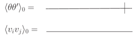
Figure 1: The graphical representation of the propagators of the model.

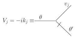
Figure 2: The interaction vertex of the model
(wave-number-frequency representation).

Action (9) is given in a form convenient for a realization of the field theoretic perturbation analysis with the standard Feynman diagrammatic technique. The matrix of bare propagators is obtained from the quadratic part of the action. The wave-number-frequency representation of, in what follows, important propagators are: a) the bare propagator $\langle\theta\theta^{\prime}\rangle_{0}$ defined as

$$\langle\theta\theta^{\prime}\rangle_{0}=\langle\theta^{\prime}\theta\rangle^{*}_{0}=\frac{1}{-i\omega+\nu_{0}k^{2}},$$ (12)

and b) the bare propagator for the velocity field $\langle vv\rangle_{0}$ given directly by (4), namely

$$\langle v_{i}v_{j}\rangle_{0}=\left(P_{ij}({\bf k})+\alpha Q_{ij}({\bf k})\right)D^{v}(\omega,k).$$ (13)

Their graphical representation is present in figure 1.

The triple (interaction) vertex $-\theta^{\prime}v_{j}\partial_{j}\theta=\theta^{\prime}v_{j}V_{j}\theta$ is present in figure 2, where momentum ${\bf k}$ is flowing into the vertex via the scalar field $\theta$.

4 Renormalization and RG analysis

The model under consideration is logarithmic at $\varepsilon=\eta=0$ (the coupling constants $g_{0}$, and $u_{0}$ are dimensionless), therefore the UV divergences in the correlation functions have the form of the poles in $\varepsilon,\eta$, and their linear combinations.

The crucial role in the renormalization of the model is played by the total canonical dimension of an arbitrary one-particle irreducible correlation (Green) function $\Gamma=\langle\Phi\cdots\Phi\rangle_{1-ir}$. It plays the role of the formal index of the UV divergence and it is given as follows [8, 9]

$$d_{\Gamma}=d^{k}_{\Gamma}+2d^{\omega}_{\Gamma}=d+2-N_{\Phi}d_{\Phi},$$ (14)

where $N_{\Phi}=\{N_{\theta},N_{\theta^{\prime}},N_{{\bf v}}\}$ are the numbers of corresponding fields entering into the function $\Gamma$, $d^{k}_{\Gamma}$ and $d^{\omega}_{\Gamma}$ are the canonical momentum dimension and the canonical frequency dimension of the function $\Gamma$, respectively, and summation over all types of fields is implied. In what follows, we shall use the definitions of the canonical dimensions of the fields $\Phi$ as they are given in [12, 13]. It is well-known that superficial UV divergences, whose removal requires counterterms, can be presented only in those Green functions $\Gamma$ for which the total canonical index $d_{\Gamma}$ is non-negative integer.

From the dimensional analysis of the model (see, e.g., [12, 13]), we conclude that for any $d$, superficial UV divergences can exist only in the 1-irreducible functions $\langle\theta^{\prime}\theta\rangle_{1-ir}$ and $\langle\theta^{\prime}\theta{\bf v}\rangle_{1-ir}$. To remove them one needs to include into the action functional the counterterm of the form $\theta^{\prime}\triangle\theta$ and $\theta^{\prime}v_{i}\partial_{i}\theta$. Their inclusion is manifested by the multiplicative renormalization of the bare parameters $g_{0},u_{0}$, and $\nu_{0}$, and the velocity field ${\bf v}$ in the action functional (9):

$$\nu_{0}=\nu Z_{\nu},\,\,\,g_{0}=g\mu^{2\varepsilon+\eta}Z_{g},\,\,\,u_{0}=u\mu^{\eta}Z_{u},\,\,\,{\bf v}\rightarrow Z_{v}{\bf v}.$$ (15)

Here, the dimensionless parameters $g,u$,and $\nu$ are the renormalized counterparts of the corresponding bare ones, $\mu$ is the renormalization mass (a scale setting parameter), and $Z_{i}=Z_{i}(g,u,\alpha),i=\nu,g,u,v$ are renormalization constants.

The renormalized action functional has the following form

$$S(\Phi)= - \frac{1}{2}\int dt_{1}\,d^{d}{\bf x_{1}}\,dt_{2}\,d^{d}{\bf x_{2}}v_{i}(t_{1},{\bf x_{1}})[D_{ij}^{v}(t_{1},{\bf x_{1}};t_{2},{\bf x_{2}})]^{-1}v_{j}(t_{2},{\bf x_{2}})$$

$$+ \int dt\,d^{d}{\bf x}\,\,\theta^{\prime}\left[-\partial_{t}\theta-Z_{2}v_{i}\partial_{i}\theta+\nu Z_{1}\triangle\theta\right],$$

where the correlator $D_{ij}^{v}$ is written in renormalized parameters (in wave-number-frequency representation)

$$\tilde{D}_{ij}^{v}(\omega,k)=\frac{\left(P_{ij}({\bf k})+\alpha Q_{ij}({\bf k})\right)g\nu^{3}\mu^{2\varepsilon+\eta}k^{4-d-2\varepsilon-\eta}}{(i\omega+u\nu\mu^{\eta}k^{2-\eta})(-i\omega+u\nu\mu^{\eta}k^{2-\eta})}.$$ (17)

By comparison of the renormalized action (4) with definitions of the renormalization constants $Z_{i}$, $i=g,u,\nu$ (15) we are coming to the relations among them:

$$Z_{\nu}=Z_{1},\,\,\,Z_{u}=Z_{1}^{-1},\,\,\,Z_{g}=Z_{2}^{2}Z_{1}^{-3},\,\,\,Z_{v}=Z_{2}.$$ (18)

The second and the third relations are consequences of the absence of the renormalization of the term with $D^{v}$ in renormalized action (4).

The issue of interest are especially multiplicatively renormalizable equal-time two-point quantities $G(r)$ (see, e.g., [13]). The example of such quantity are the equal-time structure functions

$$S_{n}(r)\equiv\langle[\theta(t,{\bf x})-\theta(t,{\bf x^{\prime}})]^{n}\rangle$$ (19)

in the inertial range, specified by the inequalities $l\sim 1/\Lambda<<r<<L=1/m$ ($l$ is an internal length). The infrared (IR) scaling behavior of the function $G(r)$ (for $r/l\gg 1$ and any fixed $r/L$)

$$G(r)\simeq\nu_{0}^{d^{\omega}_{G}}l^{-d_{G}}(r/l)^{-\Delta_{G}}R(r/L)$$ (20)

is related to the existence of IR stable fixed points of the RG equations (see next section). In (20) $d^{\omega}_{G}$ and $d_{G}$ are corresponding canonical dimensions of the function $G$, $R(r/L)$ is so-called scaling function which cannot be determined by RG equation (see, e.g., [8]), and $\Delta_{G}$ is the critical dimension defined as

$$\Delta_{G}=d_{G}^{k}+\Delta_{\omega}d_{G}^{\omega}+\gamma_{G}^{*}.$$ (21)

Here $\gamma_{G}^{*}$ is the fixed point value of the anomalous dimension $\gamma_{G}\equiv\mu\partial_{\mu}\ln Z_{G}$, where $Z_{G}$ is renormalization constant of multiplicatively renormalizable quantity $G$, i.e., $G=Z_{G}G^{R}$ [13], and $\Delta_{\omega}=2-\gamma_{\nu}^{*}$ is the critical dimension of frequency with $\gamma_{\nu}=\gamma_{1}$ which is defined further in the text (for more details see, e.g., [12, 13]).

On the other hand, the small $r/L$ behavior of the scaling function $R(r/L)$ can be studied using the Wilson OPE [8]. It shows that, in the limit $r/L\to 0$, the function $R(r/L)$ have the following asymptotic form

$$R(r/L)=\sum_{F}C_{F}(r/L)\,(r/L)^{\Delta_{F}},$$ (22)

where $C_{F}$ are coefficients regular in $r/L$. In general, the summation is implied over certain renormalized composite operators $F$ with critical dimensions $\Delta_{F}$.

In present paper we shall study only the first stage of the RG analysis, namely, the influence of compressibility of the velocity field on the stability of possible scaling regimes of the model. The influence of compressibility on the anomalous scaling (the second stage of the RG analysis) will be studied in the subsequent paper.

In what follows we shall work with two-loop approximation. But the calculation of higher-order corrections is more difficult in the models with turbulent velocity field with finite correlation time than in the cases with $\delta$-correlations in time. It is related to the fact that the diagrams for the finite correlated case involve two different dispersion laws, namely, $\omega\propto k^{2}$ for the scalar field and $\omega\propto k^{2-\eta}$ for the velocity field which complicates situation even in the one-loop approximation [12, 13]. But, as was discussed in [12, 13, 18], this difficulty can be avoided by the calculation of all renormalization constants in an arbitrary specific choice of the exponents $\varepsilon$ and $\eta$ that guarantees UV finiteness of the Feynman diagrams. From the calculational point of view the most suitable choice is to put $\eta=0$ and leave $\varepsilon$ arbitrary. Thus, the knowledge of the renormalization constants for the special choice $\eta=0$ is sufficient to obtain all important quantities as the $\gamma$-functions, $\beta$-functions, coordinates of fixed points, and the critical dimensions. But such possibility is not automatic in general. In the model under consideration, it is the consequence of an analysis which shows that in the minimal subtraction (MS) scheme, which is used in what follows, all needed anomalous dimensions are independent of the exponents $\varepsilon$ and $\eta$ in the two-loop approximation. But in the three-loop approximation this dependence can simply appear [18].

Now let us continue with renormalization of the model. The relation $S(\theta,\theta^{\prime},{\bf v},e_{0})=S^{R}(\theta,\theta^{\prime},{\bf v},e,\mu)$, where $e_{0}$ stands for the complete set of bare parameters and $e$ stands for renormalized one, leads to the relation $W(A,e_{0})=W^{R}(A,e,\mu)$ for the generating functional of connected Green functions. By application of the operator $\tilde{\cal{D}}_{\mu}\equiv\mu\partial_{\mu}$ at fixed $e_{0}$ on both sides of the latest equation one obtains the basic RG differential equation

$${\cal{D}}_{RG}W^{R}(A,e,\mu)=0,$$ (23)

where ${\cal{D}}_{RG}$ represents operation $\tilde{\cal{D}}_{\mu}$ written in the renormalized variables. Its explicit form is

$${\cal{D}}_{RG}={\cal{D}}_{\mu}+\beta_{g}(g,u)\partial_{g}+\beta_{u}(g,u)\partial_{u}-\gamma_{\nu}(g,u){\cal{D}}_{\nu},$$ (24)

where we standardly denote ${\cal{D}}_{x}\equiv x\partial_{x}$ for any variable $x$, and the RG functions (the $\beta$ and $\gamma$ functions) are given by well-known definitions and, in our case, using the relations (18) for renormalization constants, they have the following form

$$\gamma_{i} \equiv \tilde{\cal{D}}_{\mu}\ln Z_{i},\,\,\,i=1,2$$ (25)

$$\beta_{g} \equiv \mu\partial_{\mu}g=g(-2\varepsilon-\eta+3\gamma_{1}-2\gamma_{2}),$$ (26)

$$\beta_{u} \equiv \mu\partial_{\mu}u=u(-\eta+\gamma_{1}).$$ (27)

The renormalization constants $Z_{1}$, and $Z_{2}$ are determined by the requirement that one-particle irreducible Green functions $\langle\theta^{\prime}\theta\rangle_{1-ir}$ and $\langle\theta^{\prime}\theta{\bf v}\rangle_{1-ir}$ must be UV finite when are written in renormalized variables. In our case, it means that they have no singularities in the limit $\varepsilon,\eta\rightarrow 0$.

The one-particle irreducible Green function $\langle\theta^{\prime}\theta\rangle_{1-ir}$ is related to the self-energy operator $\Sigma_{\theta^{\prime}\theta}$ by the Dyson equation

$$\langle\theta^{\prime}\theta\rangle_{1-ir}=-i\omega+\nu_{0}p^{2}-\Sigma_{\theta^{\prime}\theta}(\omega,p),$$ (28)

where the self-energy operator $\Sigma_{\theta^{\prime}\theta}$ is represented by the corresponding one-particle irreducible diagrams. In the two loop approximation, it is defined by the diagrams which are shown in figure 3.

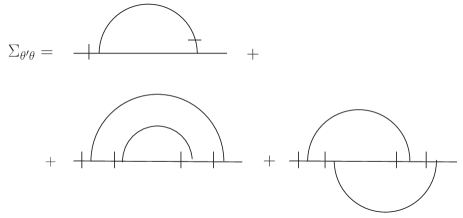
Figure 3: The one and two-loop diagrams which contribute
to the self-energy operator $\Sigma_{\theta^{\prime}\theta}$.

On the other hand, the renormalized function $\langle\theta^{\prime}\theta{\bf v}\rangle_{1-ir}$ is defined as

$$\langle\theta^{\prime}\theta v_{i}\rangle_{1-ir}=Z_{2}V_{i}+{\cal V}_{i},$$ (29)

where the function ${\cal V}_{i}$ is defined by diagrams of figure 4 (in two-loop approximation).

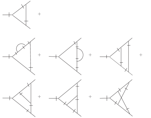
Figure 4: The one and two-loop diagrams which contribute to the function ${\cal V}_{i}$.

Thus, $Z_{1}$, and $Z_{2}$ are found from the requirement that the UV divergences are canceled in (28), and (29) after substitution $\nu_{0}=\nu Z_{\nu}=\nu Z_{1}$. This determines $Z_{1}$, and $Z_{2}$ up to an UV finite contribution, which are fixed by the choice of the renormalization scheme. In the MS scheme all renormalization constants have the form: 1 + poles in $\varepsilon,\eta$ and their linear combinations. As was already mentioned, in our calculations we can put $\eta=0$. This possibility essentially simplifies the evaluations of all quantities [12, 13, 18]. The analytical expressions for one-loop diagrams in figure 3 and figure 4 (in the MS scheme) have the following form

$$G_{1p} = -\frac{S_{d}}{(2\pi)^{d}}\frac{g\nu p^{2}}{4u(1+u)^{2}}\frac{(1+u)(d-1+\alpha)-2\alpha}{d}\left(\frac{\mu}{m}\right)^{2\varepsilon}\frac{1}{\varepsilon},$$ (30)

$$G_{1v} = i\frac{S_{d}}{(2\pi)^{d}}\frac{gp_{j}}{4u(1+u)^{2}}\frac{\alpha}{d}\left(\frac{\mu}{m}\right)^{2\varepsilon}\frac{1}{\varepsilon},$$ (31)

where $G_{1p}$ is result for the one-loop diagram in figure 3, and $G_{1v}$ is result for the one-loop diagram in figure 4. Here, $S_{d}=2\pi^{d/2}/\Gamma(d/2)$ denotes the $d$-dimensional sphere. The two-loop expressions for the diagrams in figure 3 and figure 4 are rather huge, therefore we shall not present their explicit form separately but rather we present complete expressions for renormalization constants $Z_{1}$, and $Z_{2}$ which have the following structure

$$Z_{i}=\frac{g}{\varepsilon}A_{i}+\frac{g^{2}}{\varepsilon}\left(\frac{1}{\varepsilon}B_{i}+C_{i}\right),\,\,\,i=1,2.$$ (32)

Now using the definition of the anomalous dimensions $\gamma_{1,2}$ in (25) we obtain

$$\gamma_{1} \equiv \mu\partial_{\mu}\ln Z_{1}=-2(\bar{g}A_{1}+2\bar{g}^{2}C_{1}),$$ (33)

$$\gamma_{2} \equiv \mu\partial_{\mu}\ln Z_{2}=-2(\bar{g}A_{2}+2\bar{g}^{2}C_{2}),$$ (34)

where we denote $\bar{g}=gS_{d}/(2\pi)^{d}$. The one-loop contributions $A_{1}$ and $A_{2}$ in (33) and (34) are defined as follows

$$A_{1} = -\frac{1}{4u(1+u)^{2}}\frac{(1+u)(d-1+\alpha)-2\alpha}{d},$$ (35)

$$A_{2} = \frac{\alpha}{4du(1+u)^{2}},$$ (36)

and the two-loop contributions $C_{1}$ and $C_{2}$ have the form

$$C_{1} = \frac{1}{16d^{2}u^{2}(1+u)^{3}}\left(C_{10}+\alpha C_{11}+\alpha^{2}C_{12}\right),$$ (37)

$$C_{2} = \frac{1}{32d^{3}u^{2}(1+u)^{6}}\left(\alpha C_{21}+\alpha^{2}C_{22}\right),$$ (38)

where

$$C_{10}=\frac{(d-1)(d+u)H_{2}}{(d+2)(1+u)^{2}},$$ (39)

$$C_{11}=\frac{d-1}{1+u}-\frac{u(d-1)(2+u)(2(u-2)u+d(2+3u))}{d(1+u)^{3}}H_{0}$$

$$+\frac{(d-1)(4(-2+u)u+d^{2}(-2+3u^{2}(2+u))+2d(2+u(5-5u+u^{3})))}{d^{2}(1+u)^{3}}H_{1},$$ (40)

$$C_{12}=\frac{3u-1}{(1+u)^{2}}+\frac{uH_{0}}{d(1+u)^{4}}\Big{(}2d^{2}u(1+u)^{2}-(u-3)(u-1)u(2+u)$$

$$\hskip 71.13188pt+d(2+u)(1+u(-2+(u-6)u))\Big{)}$$

$$+\frac{H_{1}}{d^{2}(1+u)^{4}}\Big{(}2(u-3)(u-1)u-2d^{3}u^{2}(1+u)^{2}$$

$$\hskip 36.98866pt-d^{2}(-1+u(5+u(2+u)(3+(u-6)u)))$$

$$\hskip 36.98866pt+d(-2+u(1+u(22+(u-4)u(2+u))))\Big{)},$$ (41)

$$C_{21}=-(d-1)d(1+u)^{2}-(d-1)du(3+5u+2u^{2})H_{0}$$

$$+(d-1)(1+2u)(2+du(2+u))H_{1}+\frac{2(d-1)d(u-1)}{d+2}H_{2},$$ (42)

$$C_{22}=-4d(1+u)$$

$$+u(-2(2+u)+d(5-2u(1+u)+d(-1+2u(1+u))))H_{0}$$

$$+\frac{2(2(1+u)-d^{3}u^{2}(1+u)^{2}+d(-3+u+5u^{2}+u^{3})+d^{2}(1-u+u^{3}+u^{4}))}{d(1+u)}H_{1}$$

$$+\frac{2d((u-1)^{2}+d(1+2u-u^{2}))}{(2+d)(1+u)}H_{2},$$ (43)

where we have used the following notation

$$H_{i}={{}_{2}F_{1}}\left[1,1;i+\frac{d}{2};\frac{1}{(1+u)^{2}}\right],\,\,\,i=0,1,2$$ (44)

for the corresponding hypergeometric function ${{}_{2}F_{1}}[a,b;c;z]=1+\frac{a\,b}{c\cdot 1}z+\frac{a(a+1)b(b+1)}{c(c+1)\cdot 1\cdot 2}z^{2}+\ldots$. The functions $B_{i},i=1,2$ which are introduced in (32) are not important in what follows, therefore we shall not define them explicitly.

5 Fixed points and scaling regimes

Possible scaling regimes of a renormalizable model are directly given by the IR stable fixed points of the corresponding system of RG equations [8, 19]. The coordinates of the fixed point of the RG equations are defined by $\beta$-functions, namely, by requirement of their vanishing. In our model the coordinates $g_{*},u_{*}$ of the fixed points are found from the system of two equations

$$\beta_{g}(g_{*},u_{*})=\beta_{u}(g_{*},u_{*})=0.$$ (45)

The beta functions $\beta_{g}$ and $\beta_{u}$ are defined in (26) and (27). The IR asymptotic behavior is governed by the IR stable fixed point which is given by the positive eigenvalues of the matrix $\Omega$ of the first derivatives:

$$\Omega_{ij}=\left(\begin{array}[]{cc}\partial\beta_{g}/\partial g&\partial\beta_{g}/\partial u\\ \partial\beta_{u}/\partial g&\partial\beta_{u}/\partial u\end{array}\right).$$ (46)

The influence of compressibility on the scaling regimes of the present model in one-loop approximation was investigated in [13]. We are interested in the answer on the following question: how can the two-loop approximation change the picture of the scaling regimes discussed in [13]?

In what follows, we shall try to study possible scaling regimes in detail. First of all, we shall investigate the rapid-change limit: $u\rightarrow\infty$. In this regime, it is necessary to make transformation to new variables, namely, $w\equiv 1/u$, and $g^{\prime}\equiv g/u^{2}$, with the corresponding changes in the $\beta$ functions:

$$\beta_{g^{\prime}} = g^{\prime}(-2\varepsilon+\eta+\gamma_{1}-2\gamma_{2}),$$ (47)

$$\beta_{w} = w(\eta-\gamma_{1}).$$ (48)

It is well-known that in the rapid change model the higher than one-loop corrections to the self-energy operator are equal to zero. On the other hand, the renormalization of the velocity field is absent at all as a consequence of the fact that $Z_{2}=1$ at all orders of the perturbation theory. It can be also seen directly by the corresponding manipulations with our $\gamma$-functions (33) and (34). Therefore, we are coming to the one-loop results of [13] (in the rapid-change model limit), namely

$$\gamma_{1}=\bar{g}^{\prime}\frac{d-1+\alpha}{2d},\,\,\,\gamma_{2}=0,$$ (49)

where again $\bar{g}^{\prime}=g^{\prime}S_{d}/(2\pi)^{d}$.

In this regime we have two fixed points denoted as FPI and FPII in [12, 13]. The first of them is trivial one

$$\mathrm{FPI}:\,\,\,\,w_{*}=g_{*}^{\prime}=0,$$ (50)

with $\gamma_{1}^{*}=0$, and diagonal matrix $\Omega$ with eigenvalues (diagonal elements)

$$\Omega_{1}=\eta,\,\,\,\,\,\Omega_{2}=\eta-2\varepsilon.$$ (51)

Thus, this fixed point is IR stable when $\eta>0$, and, at the same time, $\eta>2\varepsilon$. The second point is defined as

$$\mathrm{FPII}:\,\,\,\,w_{*}=0,\,\,\,\bar{g}_{*}^{\prime}=\frac{2d}{d-1+\alpha}(2\varepsilon-\eta),$$ (52)

with exact one loop result $\gamma_{1}^{*}=2\varepsilon-\eta$. The corresponding $\Omega$ matrix is triangular with diagonal elements (eigenvalues):

$$\Omega_{1}=2(\eta-\varepsilon),\,\,\,\,\Omega_{2}=2\varepsilon-\eta.$$ (53)

It means that this kind of the fixed point is IR stable when $\eta<2\varepsilon$ together with $\eta>\varepsilon$.

The second special case of the present model is so-called ”frozen regime” with the frozen velocity field. It is obtained from our model in the limit $u\rightarrow 0$. To consider this transition, it is again appropriate to change the variable $g$ to the new variable $g^{\prime\prime}\equiv g/u$ [12]. Then the $\beta$ functions are transform to the following ones:

$$\beta_{g^{\prime\prime}} = g^{\prime\prime}(-2\varepsilon+2\gamma_{1}-2\gamma_{2}),$$ (54)

$$\beta_{u} = u(-\eta+\gamma_{1}),$$ (55)

with unchanged $\beta$ function for parameter $u$. In this notation, the anomalous dimensions $\gamma_{1,2}$ have the form

$$\gamma_{1} = -2(\bar{g}^{\prime\prime}A_{1}^{\prime\prime}+2\bar{g}^{\prime\prime 2}C_{1}^{\prime\prime}),$$ (56)

$$\gamma_{2} = -2(\bar{g}^{\prime\prime}A_{2}^{\prime\prime}+2\bar{g}^{\prime\prime 2}C_{2}^{\prime\prime}),$$ (57)

where, as obvious, $\bar{g}^{\prime\prime}=g^{\prime\prime}S_{d}/(2\pi)^{d}$, and the one-loop contributions are now given as

$$A_{1}^{\prime\prime} = -\frac{d-1-\alpha}{4d},$$ (58)

$$A_{2}^{\prime\prime} = \frac{\alpha}{4d},$$ (59)

and the two-loop contributions $C_{1}^{\prime\prime}$ and $C_{2}^{\prime\prime}$ are now

$$C_{1}^{\prime\prime} = \frac{1}{16d^{2}}\left(C_{10}^{\prime\prime}+\alpha C_{11}^{\prime\prime}+\alpha^{2}C_{12}^{\prime\prime}\right),$$ (60)

$$C_{2}^{\prime\prime} = \frac{1}{32d^{3}}\left(\alpha C_{21}^{\prime\prime}+\alpha^{2}C_{22}^{\prime\prime}\right),$$ (61)

with

$$C_{10}^{\prime\prime}=\frac{(d-1)d}{(d+2)}H_{02}=d-1,$$ (62)

$$C_{11}^{\prime\prime}=(d-1)\left(1-\frac{2(d-2)}{d}H_{01}\right)=1-d,$$ (63)

$$C_{12}^{\prime\prime}=-1+\frac{d-2}{d}H_{01}=0,$$ (64)

$$C_{21}^{\prime\prime}=2(d-1)\left(H_{01}-\frac{d}{d+2}H_{02}\right)=\frac{4(d-1)}{d-2},$$ (65)

$$C_{22}^{\prime\prime}=\frac{2(d-1)(d-2)}{d}H_{01}+\frac{2d(1+d)}{(2+d)}H_{02}=4d,$$ (66)

where we denote

$$H_{0i}={{}_{2}F_{1}}\left[1,1;i+\frac{d}{2};1\right]=\frac{d-2+2i}{d-4+2i},\,\,\,i\geq 1.$$ (67)

The system of $\beta$ functions (54) and (55) exhibits two fixed points, denoted as FPIII and FPIV in [12]. They are related to the corresponding two scaling regimes. One of them is trivial,

$$\mathrm{FPIII}:\,\,\,\,u_{*}=g_{*}^{\prime\prime}=0,$$ (68)

with $\gamma_{1}^{*}=\gamma_{2}^{*}=0$. The eigenvalues of the corresponding matrix $\Omega$, which is diagonal in this case, are

$$\Omega_{1}=-2\varepsilon,\,\,\,\,\Omega_{2}=-\eta.$$ (69)

Thus, this regime is IR stable only if both parameters $\varepsilon$, and $\eta$ are negative simultaneously. The second, non-trivial, point is

$$\mathrm{FPIV}:\,\,\,\,u_{*}=0,\,\,\,\,\bar{g}_{*}^{\prime\prime}=-\frac{\varepsilon}{2(A_{1}^{\prime\prime}-A_{2}^{\prime\prime})}-\frac{C_{1}^{\prime\prime}-C_{2}^{\prime\prime}}{2(A_{1}^{\prime\prime}-A_{2}^{\prime\prime})^{3}}\varepsilon^{2},$$ (70)

with exact one-loop relation $\gamma_{1}^{*}=\gamma_{2}^{*}+\varepsilon$. After substitution of the corresponding quantities one obtains the following expression for the coordinates of the fixed point

$$u_{*}=0,\,\,\,\,\bar{g}_{*}^{\prime\prime}=\frac{2d\varepsilon}{d-1}\left\{1+\frac{\varepsilon}{(d-1)^{2}}\left[(d-1)\left(1-\alpha\left(1+\frac{2}{d(d-2)}\right)\right)-2\alpha^{2}\right]\right\}.$$ (71)

The eigenvalues of the matrix $\Omega$ (taken at the fixed point) are

$$\Omega_{1}=2\varepsilon\left(1-\frac{C_{1}^{\prime\prime}-C_{2}^{\prime\prime}}{(A_{1}^{\prime\prime}-A_{2}^{\prime\prime})^{2}}\varepsilon\right),\,\,\,\Omega_{2}=\varepsilon-\eta+\gamma_{2}^{*}.$$ (72)

After corresponding substitutions one has

$$\Omega_{1}=2\varepsilon\left\{1-\frac{\varepsilon}{(d-1)^{2}}\left[(d-1)\left(1-\alpha\left(1+\frac{2}{d(d-2)}\right)\right)-2\alpha^{2}\right]\right\},$$ (73)

$$\Omega_{2}=\varepsilon-\eta+\frac{\alpha\,\varepsilon}{d-1}\left[-1+\varepsilon\frac{2\alpha^{2}(d-2)d-(d-1)(d^{2}-2)-\alpha(2+(d-3)d^{2})}{(d(d-1)^{2}(d-2))}\right].$$ (74)

The conditions $\bar{g}_{*}^{\prime\prime}>0,\Omega_{1}>0$, and $\Omega_{2}>0$ for the IR stable fixed point lead to the restrictions on the values of the parameters $\varepsilon$ and $\eta$. First, suppose that $\varepsilon<0$. Then from the conditions $\bar{g}_{*}^{\prime\prime}>0$, and $\Omega_{1}>0$ one has the following restrictions which must be fulfilled simultaneously

$$1+\varepsilon D<0,\,\,\,1-\varepsilon D<0,$$ (75)

but they cannot be fulfilled at the same time. Thus, our first condition is $\varepsilon>0$. In (75) $D$ is given as

$$D=\frac{1}{(d-1)^{2}}\left[(d-1)\left(1-\alpha\left(1+\frac{2}{d(d-2)}\right)\right)-2\alpha^{2}\right].$$ (76)

To have $\bar{g}_{*}^{\prime\prime}>0$, and $\Omega_{1}>0$ together with $\varepsilon>0$, the following inequalities must be held

$$-1<\varepsilon D<1,$$ (77)

which restricts the value of $\varepsilon$ as a function of the parameter $\alpha$, and the dimension of the space $d$. In the incompressible case ($\alpha=0$) the condition (77) is reduced into the simple inequality

$$\varepsilon<d-1.$$ (78)

In the general case, for each value of $d$, there exists a ”critical” value of $\alpha$ in which $D=0$. We denote it as $\alpha_{c}$. In this situation $\varepsilon$ can be arbitrary, i.e., the condition (77) is fulfilled automatically. The value of $\alpha_{c}$ is defined as follows

$$\alpha_{c}=\frac{2-4d+3d^{2}-d^{3}+(4-16d-4d^{2}+36d^{3}-23d^{4}+2d^{5}+d^{6})^{1/2}}{4d(d-2)}.$$ (79)

For example, for $d=3$ its value is $\alpha_{c}=\frac{\sqrt{61}-5}{6}\simeq 0.468$. Therefore, in the compressible model, the situation is a little bit more complicated as a result of a competition between incompressible and compressible terms within two-loop approximation which leads to the existence of $\alpha_{c}$. How does it work? The answer is the following. If we continuously increase the value of the parameter $\alpha$, the region of stability of the fixed point defined by the inequalities (77) increases too. This restriction vanishes completely when $\alpha$ reaches the ”critical” value $\alpha_{c}$. In this rather specific situation the two-loop influence on the region of stability of fixed point defined by condition (77) is exactly zero. Then, if the value of parameter $\alpha$ increases further, the condition (77) appears again, and restriction on $\varepsilon$ becomes stronger when $\alpha$ tends, in principle, to infinity. In this limit $\varepsilon\rightarrow 0$. On the other hand, it must be stressed that in our model only relatively small values of $\alpha$ are allowed ($\alpha\ll 1$). It corresponds to small fluctuations of the density $\rho$ in the system which is supposed in our investigation. In other words, it is supposed that the stochastic component of the velocity field of the fluid is much smaller than the velocity of the sound in the system (the Mach number $Ma\ll 1$).

The last condition on the stability of the IR fixed point is found from the requirement to have $\Omega_{2}>0$. It reads

$$\eta<\varepsilon+\frac{\alpha\,\varepsilon}{d-1}\left[-1+\varepsilon\frac{2\alpha^{2}(d-2)d-(d-1)(d^{2}-2)-\alpha(2+(d-3)d^{2})}{(d(d-1)^{2}(d-2))}\right].$$ (80)

In the incompressible case it is reduced into the simple condition

$$\eta<\varepsilon,$$ (81)

which is held at each order of the perturbation theory.

In the end, let us consider the most interesting scaling regime with finite value of the fixed point for variable $u$. The coordinates of the fixed point is now defined by the requirement of vanishing of the $\beta$ functions which are given in (26) and (27). The fixed point value for $\bar{g}=gS_{d}/(2\pi)^{d}$ is given as

$$\mathrm{FPV}:\,\,\,\,\bar{g}_{*}=-\frac{\varepsilon}{2(A_{1}-A_{2})}-\frac{C_{1}-C_{2}}{2(A_{1}-A_{2})^{3}}\varepsilon^{2},$$ (82)

where the functions $A_{1},A_{2},C_{1}$, and $C_{2}$ are given in (35)-(38), and where the parameter $u$ is taken at its fixed point value $u_{*}$ which is given implicitly by the equation

$$-\eta+\gamma_{1}^{*}(u_{*})=0.$$ (83)

Using the exact relations

$$\gamma_{1}^{*}=\eta,\,\,\,\,\,\gamma_{2}^{*}=\eta-\varepsilon$$ (84)

the expression for the fixed point value of $\bar{g}$ can be rewritten as a series (expansion) of the parameter $\eta$ or a linear combination of $\eta$ and $\varepsilon$. For example, in [13], where the problem was analyzed in one-loop approximation, it was expressed as a function of $2\varepsilon-\eta$ (in our notation). In the framework of one-loop approximation it allows one to have linear dependence of $\bar{g}_{*}$ on the fixed point value of the parameter $u$. Together with another choice of the linear combination of $\eta$ and $\varepsilon$, namely $\eta-\varepsilon$ it leads also to the simple expression for the fixed point value of $u$. Thus, the coordinates of the fixed point in one-loop approximation are [13]

$$\bar{g}_{*}=\frac{2d(1+u_{*})}{d-1+\alpha}(2\varepsilon-\eta),\,\,\,\,\,\,u_{*}=-1+\frac{\alpha}{d-1+\alpha}\frac{\eta-2\varepsilon}{\eta-\varepsilon}.$$ (85)

It allows, together with the requirement of the positive eigenvalues of the corresponding matrix of the first derivatives $\Omega$, to find simple conditions for the IR stable fixed point. They are defined by inequalities $\varepsilon>0,\varepsilon>\eta$, and $\eta>\varepsilon\frac{d-1-\alpha}{d-1}$ [13].

The situation is essentially more complicated when we are working in two-loop approximation. It is given by the fact that now we have nonlinear dependence of $\bar{g}$ on the parameters $\eta$ and $\varepsilon$, and the expression for the fixed point value of $u$ is now given only implicitly in rather complicated expression containing hypergeometric functions. Another complication, which defends to analyze the problem in general, is related to the fact that contrary to the incompressible case when one has additional condition, namely $\eta=\varepsilon$, no such condition exists in compressible case under consideration. As a result, the analysis of the IR stability of the general case of the present model have to be done individually for concrete situation. It is rather cumbersome and it will be done in the subsequent work.

In what follows, let us only give the general analysis of the most interesting case when one suppose the relation $\eta=\varepsilon$. In this situation from the definition of the $\beta$ functions given in (26) and (27) one obtains the condition

$$\gamma_{2}^{*}=0.$$ (86)

Thus, in this case, the coordinates of the fixed points are given as

$$\bar{g}_{*}=-\frac{\varepsilon}{2A_{1}}-\frac{C_{1}}{2A_{1}^{3}}\varepsilon^{2},$$ (87)

$$A_{2}(u_{*})+2\bar{g}_{*}C_{2}(u_{*})=0,$$ (88)

but even in this situation the fixed point value of $u$ is defined by complicated implicit equation (88) and its exhausted analysis must be discussed separately.

6 Conclusions

We have studied the influence of compressibility on the possible IR scaling regimes of the model of a passive scalar advected by a Gaussian velocity field with finite time correlations by means of the field theoretic RG technique. The possible scaling regimes are directly connected to the existence of IR stable fixed points of the RG equations. The dependence of the fixed points on the parameter of compressibility and their IR stability is discussed. The most attention is paid to the frozen limit of the model where inequalities which define the stable IR scaling regimes are found analytically. The existence of a ”critical” value $\alpha_{c}$ of the parameter of compressibility $\alpha$ at which one of the two-loop conditions is canceled as a result of the competition between compressible and incompressible terms is discussed in detail. The main conclusion is that for the small value of parameter $\alpha$ the region of stability is not restricted considerably. It is also shown that the most general case with finite time correlations of the velocity field is more complicated within two-loop approximation and have to be consider separately once more.

References

References

- [1] Monin A S, Jaglom A M 1975 Statistical Fluid Mechanics: Mechanics of Turbulence, Vol. 2 (Cambridge: MIT Press)
- [2] Frisch U 1995 Turbulence: the legacy of A. N. Kolmogorov (Cambridge: Cambridge University Press)
- [3] Obukhov A M 1949 Izv. Akad. Nauk SSSR, Geogr. Geofiz. 13 58
- [4] Kraichnan R H 1968 Phys. Fluids 11 945
- [5] Falkovich G, Gawȩdzki K, Vergassola M 2001 Rev. Mod. Phys. 73 913
- [6] Kraichnan R H 1994 Phys. Rev. Lett. 72 1016
- [7] Adzhemyan L Ts, Antonov N V and Vasil’ev A N 1998 Phys. Rev. E 58 1823
- [8] Vasil’ev A N 1998 Quantum-Field Renormalization Group in the Theory of Critical Phenomena and Stochastic Dynamics (St. Petersburg: St. Petersburg Institute of Nuclear Physics) [in Russian; English translation: Gordon & Breach, 2004]
- [9] Adzhemyan L Ts, Antonov N V and Vasil’ev A N 1999 The Field Theoretic Renormalization Group in Fully Developed Turbulence (London: Gordon Breach)
- [10] Adzhemyan L Ts, Antonov N V, Hnatich M and Novikov S V 2000 Phys. Rev. E 63 016309
- [11] Adzhemyan L Ts and Antonov N V 1998 Phys. Rev. E 58 7381
- [12] Antonov N V 1999 Phys. Rev. E 60 6691
- [13] Antonov N V 2000 Physica D 144 370
- [14] [] Antonov N V 2000 Zap. Nauchn. Semin. POMI 269 79
- [15] Shraiman B I and Siggia E D 1994 Phys. Rev. E 49 2912
- [16] [] Shraiman B I and Siggia E D 1995 C. R. Acad. Sci., Ser. IIb: Mec., Phys., Chim., Astron. 321 279
- [17] [] Shraiman B I and Siggia E D 1996 Phys. Rev. Lett. 77 2463
- [18] Adzhemyan L Ts, Antonov N V and Honkonen J 2002 Phys. Rev. E 66 036313
- [19] Zinn-Justin J 1989 Quantum Field Theory and Critical Phenomena (Oxford: Clarendon)
- [20] Adzhemyan L Ts, Antonov N V, Barinov V A, Kabrits Yu S and Vasil’ev A N 2001 Phys. Rev. E 64 056306
- [21] [] Adzhemyan L Ts, Antonov N V, Barinov V A, Kabrits Yu S and Vasil’ev A N 2001 Phys. Rev. E 63 025303(R)