Influence of helicity on scaling regimes in the extended Kraichnan model

Abstract

We have investigated the advection of a passive scalar quantity by incompressible helical turbulent flow in the frame of extended Kraichnan model. Turbulent fluctuations of velocity field are assumed to have the Gaussian statistics with zero mean and defined noise with finite time-correlation. Actual calculations have been done up to two-loop approximation in the frame of field-theoretic renormalization group approach. It turned out that space parity violation (helicity) of turbulent environment does not affect anomalous scaling which is peculiar attribute of corresponding model without helicity. However, stability of asymptotic regimes, where anomalous scaling takes place, strongly depends on the amount of helicity. Moreover, helicity gives rise to the turbulent diffusivity, which has been calculated in one-loop approximation.

1 Introduction

During the last decade much attention has been paid to the inertial range of fully developed turbulence, which contains wave numbers larger then those that pump the energy into the system and smaller enough then those that are related to the dissipation processes [1]. Grounding of the inertial range turbulence have been created in the well known Kolmogorov–Obukhov (KO) phenomenological theory (see, e.g., [1, 2, 3]). One of the main problems in the modern theory of fully developed turbulence is to verify the validity of the basic principles of KO theory and their consequences within the framework of a microscopic model. Recent experimental and theoretical studies indicate possible deviations from the celebrated Kolmogorov scaling exponents. The scaling behavior of the velocity fluctuations with exponents, which values are different from Kolmogorov ones, is called as anomalous and usually is associated with intermittency phenomenon. Roughly speaking, intermittency means that statistical properties (for example, correlation or structure functions of the turbulent velocity field) are dominated by rare spatiotemporal configurations, in which the regions with strong turbulent activity have exotic (fractal) geometry and are embedded into the vast regions with regular (laminar) flow. In the turbulence such phenomenon is believed to be related to the strong fluctuations of the energy flux which, therefore, leads to deviations from the predictions of the aforementioned KO theory. The deviations, referred to as “anomalous” or “non-dimensional” scaling, manifest themselves in singular (arguably power-like) dependence of correlation or structure functions on the distances and the integral (external) turbulence scale $L$. The corresponding exponents are certain nontrivial and nonlinear functions of the order of the correlation function, the phenomenon referred to as “multiscaling”.

Although the theoretical description of the fluid turbulence on the basis of the ”first principles”, i.e., on the stochastic Navier-Stokes (NS) equation [1] remains essentially an open problem, considerable progress has been achieved in understanding simplified model systems that share some important properties with the real problem: shell models [4], stochastic Burgers equation [5] and passive advection by random “synthetic” velocity fields [6].

The crucial role in these studies are played by the models of advected passive scalar field [7]. A simple model of a passive scalar quantity advected by a random Gaussian velocity field, white in time and self-similar in space (the latter property mimics some features of a real turbulent velocity ensemble), the so-called Kraichnan’s rapid-change model [8], is an example. The interest to these models is based on two important facts: first, as were shown by both natural and numerical experimental investigations, the deviations from the predictions of the classical Kolmogorov-Obukhov phenomenological theory [1, 2, 3] is even more strongly displayed for a passively advected scalar field than for the velocity field itself (see, e.g., [9, 10, 11] and references cited therein), and second, the problem of passive advection is much more easier to be consider from theoretical point of view. There, for the first time, the anomalous scaling was established on the basis of a microscopic model [12], and corresponding anomalous exponents was calculated within controlled approximations [13, 14] (see also review [6] and references therein).

The greatest stimulation to study the simple models of passive advection not only of scalar fields but also of vector fields (e.g., weak magnetic field) is related to the fact that even simplified models with given Gaussian statistics of so-called ”synthetic” velocity field describes a lot of features of anomalous behavior of genuine turbulent transport of some quantities (as heat or mass) observed in experiments, see, e.g., [11]–[15] and references cited therein.

The term “anomalous scaling” reminds of the critical scaling in models of equilibrium phase transitions. In those, the field theoretic methods were successfully employed to establish the existence of self-similar (scaling) regimes and to construct regular perturbative calculational schemes (the famous $\epsilon$ expansion and its relatives) for the corresponding exponents, scaling functions, ratios of amplitudes etc; see e.g. [16, 17]. Here and below, by “field theoretic methods” we mean diagrammatic and functional techniques, renormalization theory and renormalization group, composite operators, operator-product expansion and so on [17].

The feature specific to the theory of turbulence and simplified models associated with it is the existence in the corresponding field theoretical models of the composite operators with negative scaling (critical) dimensions. Such operators, termed “dangerous” in [18, 19, 20, 21, 22], give rise to the anomalous scaling, i.e., the singular dependence on the infrared (IR) scale $L$ with certain nonlinear anomalous exponents.

Important advantages of the RG approach are its universality and calculational efficiency: a regular systematic perturbation expansion for the anomalous exponents was constructed, similar to the well-known $\epsilon$-expansion in the theory of phase transitions, and the exponents were calculated in the first order of expansion for passively advected vector fields [24, 25] and in the second [18] and third [20] orders of that expansion for scalar fields. Furthermore, the RG approach is not related only to the rapid-change model and can also be applied to the case with finite correlation time, anisotropy, the space parity violation, and, moreover, non-Gaussian advecting field [22].

The solution proceeds in two main stages. In the first stage, the multiplicative renormalizability of the corresponding field theoretic model is demonstrated and the differential RG equations for its correlation functions are obtained. The asymptotic behavior of the latter on their UV argument $(r/l)$ ($l$ is internal length) for $r\gg\ell$ and any fixed $(r/L)$ ($L$ is an outer length) is given by IR stable fixed points of those equations. It involves some “scaling functions” of the IR argument $(r/L)$, whose form is not determined by the RG equations. In the second stage, their behavior at $r\ll L$ is found from the operator product expansion within the framework of the general solution of the RG equations. There, the crucial role is played by the critical dimensions of various composite operators, which give rise to an infinite family of independent scaling exponents (and hence to multiscaling). Of course, these both stages (and thus the phenomenon of multiscaling) have long been known in the RG theory of critical behavior. The distinguishing feature, specific to the models of turbulence is the existence of composite operators with aforementioned negative critical dimensions. Their contributions to the operator product expansion diverge at $(r/L)\to 0$. In the models of critical phenomena, nontrivial composite operators always have positive dimensions and determine only corrections (vanishing for $(r/L)\to 0$) to the leading terms (finite for $(r/L)\to 0$) in the scaling functions.

Existence of regular perturbation schemes and accurate numerical simulations allows one to discuss, for the example of the rapid-change model and its descendants, the issues that are interesting within the general context of fully developed turbulence: universality and saturation of anomalous exponents, effects of compressibility, anisotropy and pressure, persistence of the large-scale anisotropy and hierarchy of anisotropic contributions and so on. Moreover, it is interesting and important to study the helicity (violation of space parity) effects because many turbulence phenomena are directly influenced by them.

In [22] the problem of a passive scalar advected by the Gaussian self-similar velocity field with finite correlation time [26] was studied by the field theoretic RG method. There, the systematic study of the possible scaling regimes and anomalous behavior was present at one-loop level. The two-loop corrections to the anomalous exponents were obtained in [28]. It was shown that the anomalous exponents are nonuniversal as a result of their dependence on a dimensionless parameter, the ratio of the velocity correlation time, and turnover time of a scalar field.

In what follows, we shall continue with the investigation of this model from the point of view of the influence of helicity on the scaling regimes and the anomalous exponents within two-loop approximation.

Helicity is defined as the scalar product of velocity and vorticity and its non zero value expresses mirror symmetry breaking of turbulent flow. It plays significant role in the processes of magnetic field generation in electrically conductive fluid [29, 30] and represents one of the most important characteristics of large-scale motions as well [31, 32]. Despite of this fact the role of the helicity in hydrodynamical turbulence is not completely clarified up to now.

The Navier-Stokes equations conserve kinetic energy and helicity in inviscid limit. Presence of two quadratic invariants leads to the possibility of appearance of double cascade. It means that cascades of energy and helicity take place in different ranges of wave numbers analogously to the two-dimensional turbulence and/or the helicity cascade appears concurrently to the energy one in the direction of small scales [34, 35, 36]. Particularly, helicity cascade is closely connected with the existence of exact relation between triple and double correlations of velocity known as “2/15” law analogously to the “4/5” Kolmogorov law [37, 38]. Corresponding to [34] aforementioned scenarios of turbulent cascades differ each other by spectral scaling. Theoretical arguments given by Kraichnan [39] and results of numerical calculations of Navier-Stokes equations [40] support the scenario of concurrent cascades. The appearance of helicity in turbulent system leads to constraint of non-linear cascade to the small scales. This phenomenon was firstly demonstrated by Kraichnan [39] within the modelling problem of statistically equilibrium spectra and later in numerical experiments.

Turbulent viscosity and diffusivity, which characterize influence of small-scale motions on heat and momentum transport, are basic quantities investigated in the theoretic and applied models. The constraint of direct energy cascade in helical turbulence has to be accompanied by decrease of turbulent viscosity. However, no influence of helicity on turbulent viscosity was found in some works [41, 42]. Similar situation is observed for turbulent diffusivity in helical turbulence. Although the modelling calculations demonstrate intensification of turbulent transfer in the presence of helicity [43] direct calculation of diffusivity does not confirm this effect [44, 45]. Helicity is the pseudoscalar quantity hence it can be easily understood, that its influence appears only in quadratic and higher terms of perturbation theory or in the combination with another pseudoscalar quantities (e.g., large-scale helicity). Really, simultaneous consideration of memory effects and second order approximation indicate effective influence of helicity on turbulent viscosity [46] and turbulent diffusivity [43, 47, 48] already in the limit of small or infinite correlation time.

Helicity, as we shall see below, does not affect known results in one-loop approximation and, therefore, it is necessary to turn to the second order (two-loop) approximation to be able to analyze possible consequences. It is also important to say that in the framework of classical Kraichnan model, i.e., the model of passive advection by the Gaussian velocity field with $\delta$-like correlations in time, it is not possible to study the influence of the helicity because all potentially ”helical” diagrams are identically equal to zero at all orders in the perturbation theory. In this sense, the investigation of the helicity in the present model can be consider as the first step to analyze the helicity in genuine turbulence.

2 Field theoretic description of the model

The advection of a passive scalar field $\theta(x)\equiv\theta(t,\mathbf{x})$ in helical turbulent environment is described by the stochastic equation

$$\partial_{t}\theta+v_{i}\partial_{i}\theta=\nu_{0}\Delta\theta+f,$$ (1)

where $\partial_{t}\equiv\partial/\partial t$, $\partial_{i}\equiv\partial/\partial\mathrm{x}_{i}$, $\nu_{0}$ is the molecular diffusivity coefficient (hereafter all parameters with a subscript $0$ denote bare parameters of unrenormalized theory; see below), $\triangle\equiv\partial^{2}$ is the Laplace operator, $v_{i}\equiv v_{i}(x)$ is the $i$-th component of the divergence-free (owing to the incompressibility) velocity field ${\bf v}(x)$, and $f\equiv f(x)$ is an artificial the Gaussian random noise with zero mean and correlation function

$$\langle f(x)f(x^{\prime})\rangle=\delta(t-t^{\prime})C(\mathbf{r}/L),\,\,\,\mathbf{r}=\mathbf{x}-\mathbf{x}^{\prime},$$ (2)

where $L$ denotes an integral (outer) scale. It maintains the steady-state of the system but the detailed form of the function $C(\mathbf{r}/L)$ is unessential in our consideration. In spite of the fact that in real problems the velocity field ${\bf v}(x)$ satisfies the Navier-Stokes equation, in what follows, we suppose that the statistics of velocity field is given in the form of Gaussian distribution with zero mean and correlator

$$\langle v_{i}(x)v_{j}(x^{\prime})\rangle=\int\frac{\mathrm{d}\omega d^{d}k}{(2\pi)^{d+1}}P^{\rho}_{ij}({\bf k})D_{v}(\omega,k)\exp[-i\omega(t-t^{\prime})+i{\bf k}({\bf x}-{\bf x^{\prime}})],$$ (3)

with

$$D_{v}(\omega,k)=\frac{D_{0}k^{4-d-2\varepsilon-\eta}}{(i\omega+u_{0}\nu_{0}{k}^{2-\eta})(-i\omega+u_{0}\nu_{0}k^{2-\eta})},$$ (4)

where $k=|\mathbf{k}|$, $D_{0}=\mathrm{g}_{0}\nu_{0}^{3}$ is a positive amplitude factor, $\mathrm{g}_{0}$ plays the role of the coupling constant of the model, an analog of the coupling constant $\lambda_{0}$ in the $\lambda_{0}\varphi^{4}$ model of critical behavior [16, 17]. In addition, $\mathrm{g}_{0}$ is a formal small parameter of the ordinary perturbation theory. The positive exponents $\varepsilon$ and $\eta$ ($\varepsilon=O(\eta)$) are small RG expansion parameters, the analogs of the parameter $\varepsilon=4-d$ in the $\lambda_{0}\varphi^{4}$ theory. Thus we have a kind of double expansion model in the $\varepsilon-\eta$ plane around the origin $\varepsilon=\eta=0$. The correlator (4) is directly related to the energy spectrum via the frequency integral [22]

$$E(k)\simeq k^{d-1}\int\mathrm{d}\omega D^{v}(\omega,k)\simeq\frac{\mathrm{g}_{0}\nu_{0}^{2}}{u_{0}}k^{1-2\varepsilon}.$$ (5)

Therefore, the coupling constant $\mathrm{g}_{0}$ and the exponent $\varepsilon$ describe the equal-time velocity correlator or, equivalently, energy spectrum. On the other hand, the constant $u_{0}$ and the second exponent $\eta$ are related to the frequency $\omega\simeq u_{0}\nu_{0}k^{2-\eta}$ which characterizes the mode $\mathbf{k}$ [49]. Thus, in our notation, the value $\varepsilon=4/3$ corresponds to the well-known Kolmogorov ”five-thirds law” for the spatial statistics of velocity field, and $\eta=4/3$ corresponds to the Kolmogorov frequency. For completeness, we remain $d$-dependence in expressions (3) and (4) ($d$ is the dimensionality of the ${\bf x}$ space), although, of course, when one investigates system with helicity the dimension of the ${\bf x}$ space must be strictly equal to three. To include helicity the transverse projector $P^{\rho}_{ij}({\bf k})$ is taken in the form

$$P^{\rho}_{ij}({\bf k})=P_{ij}({\bf k})+H_{ij}({\bf k})=\delta_{ij}-k_{i}k_{j}/k^{2}+i\rho\epsilon_{ijl}\frac{k_{l}}{k}.$$ (6)

Here $P_{ij}({\bf k})=\delta_{ij}-k_{i}k_{j}/k^{2}$ represents non-helical part of the total transverse projector $P^{\rho}_{ij}({\bf k})$. On the other hand, $H_{ij}({\bf k})=i\rho\epsilon_{ijl}k_{l}/k$ mimics the presence of helicity in the flow. Thus, formally, the transition to the helical fluid corresponds to the breaking of spatial parity, and, technically, this is expressed by the fact that the correlation function is specified in the form of mixture of a true tensor and a pseudotensor. The tensor $\varepsilon_{ijl}$ is Levi-Civita’s completely antisymmetric tensor of rank 3 and the real parameter $\rho$, characterizes the amount of helicity. Due to the requirement of positive definiteness of the correlation function the absolute value of $\rho$ must be in the interval $|\rho|\in\langle 0,1\rangle$. Non-zero helical part proportional to $\rho$ physically expresses existence of non-zero correlations $\langle{\bf v}\cdot\mathrm{rot}\>{\bf v}\rangle$.

The general model (3), (4) contains two important special cases: rapid-change model limit when $u_{0}\rightarrow\infty$ and $\mathrm{g}_{0}^{\prime}\equiv\mathrm{g}_{0}/u_{0}^{2}=$ const, $D_{v}(\omega,k)\rightarrow\mathrm{g}_{0}^{\prime}\nu_{0}k^{-d-2\varepsilon+\eta},$ and quenched (time-independent or frozen) velocity field limit which is defined by $u_{0}\rightarrow 0$ and $\mathrm{g}_{0}^{\prime\prime}\equiv\mathrm{g}_{0}/u_{0}=$ const, $D_{v}(\omega,k)\rightarrow\mathrm{g}_{0}^{\prime\prime}\nu_{0}^{2}\pi\delta(\omega)k^{-d+2-2\varepsilon},$ which is similar to the well-known models of the random walks in random environment with long range correlations; see, e.g., [50, 51].

Using Martin-Siggia-Rose mechanism [52] the stochastic problem (1)-(4) can be treated as a field theory with action functional

$$S(\theta,\theta^{\prime},\mathbf{v})=\theta^{\prime}D_{\theta}\theta^{\prime}/2+\theta^{\prime}[-\partial_{t}+\nu_{0}\triangle-(v_{i}\partial_{i})]\theta-\mathbf{v}D_{v}^{-1}\mathbf{v}/2,$$ (7)

where $\theta^{\prime}$ is an auxiliary scalar field, and $D_{\theta}$ and $D_{v}$ are correlators (2) and (3), respectively. In the action (7) all the required integrations over $x=(t,\mathbf{x})$ and summations over the vector indices are understood. The first four terms in Eq. (7) represent the Dominicis-Jansen type action for the stochastic problem (1), (2) at fixed $\mathbf{v}$, and the last term represents the Gaussian averaging over $\mathbf{v}$.

The model (7) corresponds to a standard Feynman diagrammatic technique with the bare propagators $\langle\theta\theta^{\prime}\rangle_{0}$ and $\langle v_{i}v_{j}\rangle_{0}$ (in the momentum-frequency representation)

$$\langle\theta(\omega,{\mathbf{k}})\theta^{\prime}(\omega,{\mathbf{k}})\rangle_{0}=\frac{1}{-i\omega+\nu_{0}k^{2}},\,\langle v_{i}(\omega,{\mathbf{k}})v_{j}(\omega,{\mathbf{k}})\rangle_{0}=P^{\rho}_{ij}(\mathbf{k})D_{v}(\omega,k),$$ (8)

where $D_{v}(\omega,k)$ is given directly by (4). In the Feynman diagrams, these propagators are represented by the lines which are shown in figure 1 (the end with a slash in the propagator $\langle\theta\theta^{\prime}\rangle_{0}$ corresponds to the field $\theta^{\prime}$, and the end without a slash corresponds to the field $\theta$). The triple vertex (or interaction vertex) $-\theta^{\prime}v_{j}\partial_{j}\theta=\theta^{\prime}v_{j}V_{j}\theta$, where $V_{j}=ik_{j}$ (in the momentum-frequency representation), is presented in figure 1, where momentum $\mathbf{k}$ is flowing into the vertex via the auxiliary field $\theta^{\prime}$.

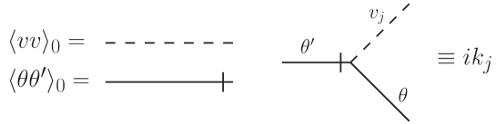
Figure 1: (Left) Graphical representations of the needed propagators of the model. (Right) The triple (interaction) vertex of the model. Momentum ${\mathbf{k}}$ is entering into the vertex via field $\theta^{\prime}$.

3 Renormalization group analysis

The model (7) is logarithmic for $\epsilon=\eta=0$ (the coupling constant $\mathrm{g}_{0}$ is dimensionless) and, in this case, possible ultraviolet (UV) divergences have the form of poles in various linear combinations of $\varepsilon$ and $\eta$ in the correlation functions. Using the standard analysis of quantum field theory one finds that all divergences can be removed by the only counterterm of the form $\theta^{\prime}\triangle\theta$ [22]. Thus, the model is multiplicatively renormalizable, which is expressed explicitly in the multiplicative renormalization of the parameters $\mathrm{g}_{0},u_{0}$, and $\nu_{0}$ in the form

$$\nu_{0}=\nu Z_{\nu},\,\,\,\mathrm{g}_{0}=\mathrm{g}\mu^{2\varepsilon+\eta}Z_{\mathrm{g}},\,\,\,u_{0}=u\mu^{\eta}Z_{u}.$$ (9)

Here the dimensionless parameters $\mathrm{g},u$ and $\nu$ are the renormalized counterparts of the corresponding bare ones, $\mu$ is the renormalization mass (a scale setting parameter), an artefact of dimensional regularization. Newly introduced quantities $Z_{i}=Z_{i}(\mathrm{g},u;d,\rho;\varepsilon,\eta)=Z_{i}(\mathrm{g},u;d,\rho;\varepsilon)$ are renormalization constants (note that if $\rho$ is non-zero then $d=3$) and, in general, contain poles of linear combinations of $\varepsilon$ and $\eta.$ However, as detailed analysis shows, to obtain all important quantities as the $\gamma$-functions, $\beta$-functions, coordinates of fixed points, and the critical dimensions, the knowledge of the renormalization constants for the special choice $\eta=0$ is sufficient up to two-loop approximation (see details in [22]).

The renormalized action functional has the following form

$$S_{R}(\theta,\theta^{\prime},\mathbf{v})=\theta^{\prime}D_{\theta}\theta^{\prime}/2+\theta^{\prime}[-\partial_{t}+\nu Z_{1}\triangle-(v\partial)]\theta-\mathbf{v}D_{v}^{-1}\mathbf{v}/2,$$ (10)

where the correlator $D_{v}$ is written in renormalized parameters. By comparison of the renormalized action (10) with definitions of the renormalization constants $Z_{i}$, $i=\mathrm{g},u,\nu$ (9) one comes to the relations among them:

$$Z_{\nu}=Z_{1},\,\,\,Z_{\mathrm{g}}=Z_{\nu}^{-3},\,\,\,Z_{u}=Z_{\nu}^{-1}.$$ (11)

The second and third relations are consequences of the absence of the renormalization of the term with $D_{v}$ in renormalized action (10). The parameter $\rho$ a the fields $\theta,\theta^{\prime},\mathbf{v}$ are not renormalized therefore $Z_{\rho}=Z_{\theta}=Z_{\theta^{\prime}}=Z_{\mathbf{v}}=1$.

The issue of interest is, in particular, the behavior of the equal-time structure functions

$$S_{n}(r)\equiv\langle[\theta(t,{\bf x})-\theta(t,{\bf x^{\prime}})]^{n}\rangle,\qquad\,r\equiv|\mathbf{r}|=|\mathbf{x}-\mathbf{x}^{\prime}|$$ (12)

in the inertial range, specified by the inequalities $l<<r<<L$ ($l$ is internal length). Here parentheses $<>$ mean the functional average over the fields $\theta,\theta^{\prime},{\bf v}$ with the weight $exp(S_{R}).$ In the isotropic case, the odd functions $S_{2n+1}$ vanish, while for $S_{2n}$ simple dimensionality considerations give

$$S_{2n}(r)=\nu_{0}^{-n}\,r^{2n}\,R_{2n}(r/l,r/L,\mathrm{g}_{0},u_{0},\rho),$$ (13)

where $R_{2n}$ are some functions of dimensionless variables. In principle, they can be calculated within the ordinary perturbation theory (i.e., as series in $\mathrm{g}_{0}$), but this is not useful for studying inertial-range behavior: the coefficients are singular in the limits $\ r/l\to\infty$ and/or $r/L\to 0$, which compensate the smallness of $\mathrm{g}_{0}$, and in order to find correct infrared behavior we have to sum the entire series. The desired summation can be accomplished using the field theoretic renormalization group (RG) and operator product expansion (OPE); see [18, 20, 22] for details.

The RG analysis consists of two main stages. On the first stage, the multiplicative renormalizability of the model is demonstrated and the differential RG equations for its correlation (structure) functions are obtained. The asymptotic behavior of the functions like (12) for $r/l>>1$ and any fixed $r/L$ is given by IR stable fixed points $\mathrm{g}_{*},u_{*}$ (see below) of the RG equations and has the form

$$S_{2n}(r)=\nu_{0}^{-n}\,r^{2n}\,(r/l)^{-\gamma_{n}}R_{2n}(r/L,\rho),\quad r/l>>1$$ (14)

with certain, as yet unknown, scaling functions $R_{2n}(r/L,\rho)\equiv R_{2n}(1,r/L,\mathrm{g}_{*},u_{*},\rho)$. In the theory of critical phenomena [16, 17] the quantity $\Delta[S_{2n}]\equiv-2n+\gamma_{n}$ is termed the critical dimension, and the exponent $\gamma_{n}$, the difference between the critical dimension $\Delta[S_{2n}]$ and the canonical dimension $-2n$, is called the anomalous dimension.

On the second stage, the small $r/L$ behavior of the functions $R_{2n}(r/L,\rho)$ is studied within the general representation (14) using the operator product expansion (OPE). It shows that, in the limit $r/L\to 0$, the functions $R_{2n}(r/L,\rho)$ have the asymptotic forms

$$R_{2n}(r/L)=\sum_{F}C_{F}(r/L)\,(r/L)^{\Delta_{n}},$$ (15)

where $C_{F}$ are coefficients regular in $r/L$. In general, the summation is implied over certain renormalized composite operators $F$ with critical dimensions $\Delta_{n}$. In case under consideration the leading operators $F$ have the form $F_{n}=(\nabla_{i}\theta\nabla_{i}\theta)^{n}.$

We have performed the complete two-loop calculation of the critical dimensions of the composite operators $F_{n}$ for arbitrary values of $n$, $d$, $u$ and $\rho$ and obtain them in the following form:

$$\Delta_{n}=\Delta_{n}^{(1)}\epsilon+\Delta_{n}^{(2)}\epsilon^{2}\,,\qquad\Delta_{n}^{(1)}=\frac{-n(n-2)(d-1)}{2(d-1)(d+2)}$$ (16)

where $\Delta_{n}^{(1)}$ is critical dimension obtained in one-loop approximation. Interesting technical details of these two-loop calculations will be present elsewhere.

Two-loop contribution $\Delta_{n}^{(2)}$ is rather cumbersome and can be found in [28]. The main and interesting result consists in the fact that although separated two-loop Feynman graphs of operators $F_{n}$ strongly depend on helicity parameter $\rho$, such dependence disappears in their sum, which gives rise to the critical dimensions $\Delta_{n}$. We can conclude that in two-loop approximation anomalous scaling with negative exponents (16) is not affected by the existence of non-zero helical correlations $\langle{\bf v}rot{\bf v}\rangle$ in turbulent incompressible flow. It turns out, however, that region of stability of possible asymptotic regimes governed by fixed points of RG equations, where anomalous scaling takes place, and effective diffusivity strongly depend on $\rho$.

Let us analyze asymptotic regimes in detail. The structure functions and the other statistical averages of random fields $\theta,\theta^{\prime}$ satisfy linear differential RG equations with linear differential operator ${\cal{D}}_{RG}:$

$${\cal{D}}_{RG}={\cal{D}}_{\mu}+\beta_{\mathrm{g}}(\mathrm{g},u)\partial_{\mathrm{g}}+\beta_{u}(\mathrm{g},u)\partial_{u}-\gamma_{\nu}(\mathrm{g},u){\cal{D}}_{\nu}\,.$$ (17)

Here ${\cal{D}}_{x}\equiv x\partial_{x}$ stands for any variable $x$ and the RG functions (the $\beta$ and $\gamma$ functions) are given by well-known definitions and in our case, using the relations (11) for the renormalization constants, they acquire the following form

$$\gamma_{\nu} \equiv \tilde{\cal{D}}_{\mu}\ln Z_{\nu},$$ (18)

$$\beta_{\mathrm{g}} \equiv \tilde{\cal{D}}_{\mu}\mathrm{g}=\mathrm{g}(-2\varepsilon-\eta+3\gamma_{\nu}),$$ (19)

$$\beta_{u} \equiv \tilde{\cal{D}}_{\mu}u=u(-\eta+\gamma_{\nu}).$$ (20)

The renormalization constant $Z_{\nu}$ is determined by the requirement that response function $G\equiv\langle\theta\theta^{\prime}\rangle$ must be UV finite when is written in renormalized variables. In our case it means that it has no singularities in the limit $\varepsilon,\eta\rightarrow 0$. The response function $G$ is related to the self-energy operator $\Sigma$, which is expressed via Feynman graphs, by the Dyson equation. In frequency-momentum representation it has the following form

$$G(\omega,\mathbf{p})=\frac{1}{-i\omega+\nu_{0}p^{2}-\Sigma(\omega,\mathrm{p})}.$$ (21)

Thus, $Z_{\nu}$ is found from the requirement that the UV divergences are canceled in (21) after substitution $\nu_{0}=\nu Z_{\nu}$. This determines $Z_{\nu}$ up to an UV finite contribution, which is fixed by the choice of the renormalization scheme. In the MS scheme all the renormalization constants have the form: 1 + poles in $\varepsilon,\eta$ and their linear combinations. In contrast to the rapid-change model, where only one-loop diagram exists (it is related to the fact that all higher-order loop diagrams contain at least one closed loop which is built on by only retarded propagators, thus are automatically equal to zero), in the case with finite correlations in time of the velocity field, higher-order corrections are non-zero. In two-loop approximation the self-energy operator $\Sigma$ is defined by diagrams which are shown in figure 2.

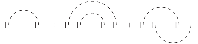
Figure 2: The one and two-loops contributions to the self-energy operator $\Sigma$.

As was already mentioned, in our calculations we can put $\eta=0$. This possibility essentially simplifies the evaluations of all quantities [22, 28].

Two-loop calculations of divergent parts of diagrams in figure 2 give the renormalization constant $Z_{\nu}$ and anomalous dimension $\gamma_{\nu}$ (18) in the form:

$$Z_{\nu}=1+\frac{g}{\varepsilon}{\cal A}+\frac{g^{2}}{\varepsilon}{\cal B}+\frac{g^{2}}{\varepsilon^{2}}{\cal C}\,,\,\gamma_{\nu}=-2(g{\cal A}+2g^{2}{\cal B}).$$ (22)

Here ${\cal A}=(1-d)/(2d(1+u))$ is the one-loop contribution to the constant $Z_{\nu}$ and anomalous dimension $\gamma_{\nu}$ and the two-loop ones are

$${\cal B} = \frac{(d-1)(d+u)}{4d^{2}(d+2)(1+u)^{5}}\,\cdot\,{{}_{2}F_{1}}\left(1,1;2+\frac{d}{2};\frac{1}{(1+u)^{2}}\right)$$ (23)

$$-\frac{\pi\rho^{2}}{36(1+u)^{3}}\,\cdot\,{{}_{2}F_{1}}\left(\frac{1}{2},\frac{1}{2};\frac{5}{2};\frac{1}{(1+u)^{2}}\right),$$

$${\cal C} = -\frac{(d-1)^{2}}{d^{2}}\frac{1}{8(1+u)^{3}}\,,$$

where ${{}_{2}F_{1}}(a,b,c,z)=1+\frac{a\,b}{c\cdot 1}z+\frac{a(a+1)b(b+1)}{c(c+1)\cdot 1\cdot 2}z^{2}+\ldots$ represents the hypergeometric function. We substitute $d=3$ in the helical part (proportional to the $\rho$), but for completeness we remain the $d$-dependence in the non-helical one. In addition we have introduced new notation $g=\mathrm{g}S_{d}/(2u(2\pi)^{d})$ ($S_{d}=2\pi^{d/2}/\Gamma(d/2)$ denotes the $d$-dimensional sphere).

From the expressions (18) - (20) and (22) we are able to find and clasify all fixed points $g_{*},u_{*}$ which satisfy equations:

$$\beta_{g}(g_{*},u_{*})=\beta_{u}(g_{*},u_{*})=0.$$ (24)

To investigate the infrared stability of a fixed point it is enough to analyze the eigenvalues of the $2\times 2$ matrix $\Omega$ of first derivatives: $\Omega_{ij}=\partial\beta_{g_{i}}/\partial g_{j}$ $(g_{i}\equiv g,u).$ The anomalous scaling is governed by the infrared stable fixed points, i.e., those for which both eigenvalues are positive.

Classification and detailed analysis of all fixed points, determination of region of their stability and influence of helicity will be present elsewhere. Here we confine ourselves to the most interesting IR stable fixed point, where both parameters $g_{*},u_{*}$ acquire non-trivial values at $\eta=\varepsilon$:

$$g_{*} = \left((g_{*}^{(1)}+\left(g_{*}^{(2)}+g_{*}^{(3)}\rho^{2}\right)\varepsilon\right)\varepsilon,\quad g_{*}^{(1)}=\frac{3}{2}(1+u_{*})\,,$$

$$g_{*}^{(2)} = \frac{3(3+u_{*})}{20(1+u_{*})^{2}}\,\cdot\,{{}_{2}F_{1}}\left(1,1;\frac{7}{2};\frac{1}{(1+u_{*})^{2}}\right)\,,$$ (25)

$$g_{*}^{(3)} = -\frac{3\pi}{8}\,\cdot\,{{}_{2}F_{1}}\left(\frac{1}{2},\frac{1}{2};\frac{5}{2};\frac{1}{(1+u_{*})^{2}}\right).$$ (26)

Actually, the equation (25) represents a line of fixed points in $g-u$ plane. The competition between helical and non-helical terms appears which yields a nontrivial restriction for the fixed point values of variable $u$ to have positive fixed values for variable $g$.

4 Effective diffusivity

One of the interesting object from the theoretical as well as experimental point of view is so-called effective diffusivity $\bar{\nu}$. In this section let us briefly investigate the effective diffusivity $\bar{\nu}$, which replaces initial molecular diffusivity $\nu_{0}$ in (1) due to the interaction of the scalar field $\theta$ with random velocity field $\mathbf{v}$. Molecular diffusivity $\nu_{0}$ governs exponential dumping in time all fluctuations in the system in the lowest approximation, which is given by the propagator (response function) (8). Analogously, the effective diffusivity $\bar{\nu}$ governs exponential dumping of all fluctuations described by full response function, which is defined by Dyson equation (21). Its explicit expression can be obtained by the RG approach. In accordance with general rules of the RG (see, e.g., [17]) all principal parameters of the model $\mathrm{g}_{0},u_{0}$ and $\nu_{0}$ are replaced by their effective (running) counterparts, which satisfy RG flow equations

$$s\frac{d\bar{g}}{ds}=\beta_{\mathrm{g}}(\bar{g},\bar{u})\,,\qquad s\frac{d\bar{u}}{ds}=\beta_{u}(\bar{g},\bar{u})\qquad s\frac{d\bar{\nu}}{ds}=-\bar{\nu}\gamma_{\nu}(\bar{g},\bar{u})$$ (27)

with initial conditions $\bar{g}|_{s=1}=g,\bar{u}|_{s=1}=u,\bar{\nu}|_{s=1}=\nu$. Here $s=k/\mu$, $\beta$ and $\gamma$ functions are defined in (18)–(20) and the running parameters $\bar{g},\bar{u}$, and $\bar{\nu}$ clearly depend on variable $s$. Due to special form of $\beta$-functions (19), (20) we are able to solve the last equation (27) analytically. Using the first equation (27) and (19) one immediately rewrites the equation for effective diffusivity in the form

$$\frac{d\bar{\nu}}{\bar{\nu}}=\frac{\gamma_{\nu}}{2\varepsilon+\eta-3\gamma_{\nu}}\frac{d\bar{g}}{\bar{g}}$$ (28)

which can be easily integrated. Using initial conditions the solution acquires the form:

$$\bar{\nu}=(\frac{g\nu^{3}}{\bar{g}s^{2\epsilon+\eta}})^{1/3}=(\frac{D_{0}}{\bar{g}k^{2\epsilon+\eta}})^{1/3}\,.$$ (29)

We emphasize that above solution is exact, i.e., the exponent $2\epsilon+\eta$ is exact too. However, in infrared region $k\ll\mu\sim l^{-1}$, $\bar{g}\rightarrow g_{*},$ which can be calculated only pertubatively. In the two-loop approximation $g_{*}=g^{(1)}_{*}\varepsilon+\left(g^{(2)}_{*}+g^{(3)}_{*}\right)\varepsilon^{2}$ and after Taylor expansion of $g_{*}^{1/3}$ in (29) we obtain:

$$\bar{\nu}\approx\nu_{*}\left(\frac{D_{0}}{g_{*}^{(1)}\varepsilon}\right)^{1/3}k^{-\frac{2\epsilon+\eta}{3}}\,,\qquad\nu_{*}\equiv 1-\frac{(g_{*}^{(2)}+g_{*}^{(3)})\varepsilon}{3g_{*}^{(1)}}\,.$$ (30)

Remind that for Kolmogorov values $\varepsilon=\eta=4/3$ the exponent in (30) becomes equal to $-4/3.$ Let us estimate the contribution of helicity to the effective diffusivity in the fixed point (25). In this point $\varepsilon=\eta$ $((2\varepsilon+\eta)/3=\varepsilon)$ and

$$\nu_{*} = 1-\varepsilon\bigg{[}(\frac{(3+u_{*})}{30(1+u_{*})^{3}}\,\cdot\,{{}_{2}F_{1}}\left(1,1;\frac{7}{2};\frac{1}{(1+u_{*})^{2}}\right)$$ (31)

$$- \frac{\pi\rho^{2}}{12(1+u_{*})}\,\cdot\,{{}_{2}F_{1}}\left(\frac{1}{2},\frac{1}{2};\frac{5}{2};\frac{1}{(1+u_{*})^{2}}\right)\bigg{]}.$$

Figure 3: (Left) The dependence of $\nu_{*}$ on the helicity parameter $\rho$ for definite IR fixed point values $u_{*}$ of the parameter $u$. (Right) The dependence of $\nu_{*}$ on the IR fixed point $u_{*}$ for the concrete values of the helicity parameter $\rho$. The value $\rho_{c}=4/\sqrt{3}$. It is a special value related to the analysis of the stability of the scaling regime which is not discussed here.

In figure 3, the dependence of the $\nu_{*}$ on the helicity parameter $\rho$ and the IR fixed point $u_{*}$ for Kolmogorov value of parameter $\varepsilon$ is shown . As one can see from these figures when $u_{*}\rightarrow\infty$ (the rapid change model limit) the two-loop corrections to $\nu_{*}=1$ are vanishing. Such behavior is related to the fact that within the rapid change model there are no two and higher loop corrections at all. On the other hand, the largest two-loop corrections to the $\nu_{*}$ are given in the frozen velocity field limit ($\nu_{*}\rightarrow 0$).

Finally, let us analyze time-behaviour of retarded response function $G\equiv<\theta\theta^{\prime}>$ in the limit $t\to\infty$.

In frequency-wave vector representation $G(\omega,{\mathbf{p}})$ satisfies Dyson equation (21). Self-energy operator $\Sigma$ is expressed via multi-loop Feynman graps and can be calculated perturbatively. We have found its divergent part up to two-loop approximation and calculated its finite part with the one-loop precision.

Using Dyson equation we find response function in time-wave vector representation:

$$G(t,\mathbf{p})=\int\frac{\mathrm{d}\omega}{2\pi}e^{-i\omega t}G(\omega,\mathbf{p})=\int\frac{\mathrm{d}\omega}{2\pi}\frac{e^{-i\omega t}}{-i\omega+\nu_{0}p^{2}-\Sigma(\omega,\mathbf{p})}\,.$$ (32)

In the lowest approximation $\Sigma(\omega,\mathbf{p})=0$, thus the integral can be easily calculated: $G_{0}(t,\mathbf{p})=\theta(t)\exp^{-i\omega_{r}t}.$ Here $\theta(t)$ denotes usual step function and $\omega_{r}$ is residuum in complex plain $\omega$ in point $-i\nu_{0}p^{2}$. According to [53], where analogical problem have been analyzed for turbulent viscosity, we suppose that this situation remains the same for the full response function $G$, i.e., the leading contribution to its asymptotic behavior for $t\to\infty$ is determined by the residuum $\omega=\omega_{r}$, which corresponds to the smallest root of dispersion relation

$$G^{-1}(\omega,\mathbf{p})=-i\omega_{r}+\nu_{0}p^{2}-\Sigma(\omega_{r},\mathbf{p})=0.$$ (33)

It is advantageous to rewrite the last relation in dimensionless form:

$$1-z-I(1,z)=0\,,\quad z\equiv\frac{i\omega_{r}}{\nu_{0}p^{2}}\,,\quad I(1,z,g)\equiv\frac{\Sigma(\omega,\mathbf{p})}{\nu_{0}p^{2}}\,,$$ (34)

which after renormalization can be rewritten in the fixed point $g_{*}$ (25) as follows

$$1-z_{*}-I_{*}=0\,,\qquad\quad z_{*}\equiv\frac{i\omega_{r}}{\bar{\nu}p^{2}}\,,$$ (35)

where $\bar{\nu}$ is effective diffusivity (30) and $I_{*}\equiv I_{*}(1,z_{*},g_{*})$ is renormalized (finite) part of dimensionless self-energy operator $I$ at the fixed point $g_{*}$.

Hence decay law $G_{0}(t,\mathbf{p})\sim\exp^{-\nu_{0}p^{2}t}$ is changed into

$$G(t,\mathbf{p})\sim\exp^{-i\omega_{r}t}=\exp^{-z_{*}\bar{\nu}p^{2}t}\,\qquad t\to\infty\,.$$ (36)

To find the residuum $\omega_{r}$ (or, equivalently, $z_{*}$) it is necessary to calculalate quantity $I_{*}$. In one-loop (linear in $\varepsilon$) approximation it can be written in the form:

$$I_{*}=-g_{*}\int_{-1}^{1}(1-x^{2})^{\frac{d-1}{2}}\mathrm{d}x\,{\cal I}\,$$ (37)

with

$${\cal I}=\int_{0}^{\infty}\mathrm{d}k\left[\frac{k}{1-z_{*}+(1+u_{*})k^{2}-2kx}-\frac{\theta(k-1)}{(1+u_{*})k}\right]\,.$$ (38)

Generally, the root $z_{*}$ can be complex and in one-loop approximation it has form

$$z^{*}=z_{1}^{*}+\mathrm{i}z_{2},\quad z_{1}^{*}=1+x_{1}\varepsilon,\quad z_{2}^{*}=x_{2}\varepsilon\,.$$ (39)

With our guaranteed precission $I_{*}$ is linear in $\varepsilon$, therefore on the first sight it seems that in the last integral it is enought to take $z_{*}=1$ ($g_{*}\sim\varepsilon$), but, actually, for its correct calculation we need to remain imaginary part $x_{2}\varepsilon.$ Then the integral (38) can be easily calculated by means of Sokhotsky’s formula:

$$\lim_{\varepsilon\rightarrow 0^{+}}\frac{1}{y\pm\mathrm{i}\epsilon}=\mp\mathrm{i}\pi\delta(y)+P(\frac{1}{y}),$$ (40)

where $P(\frac{1}{y})$ denotes the principal value of the integral. Integration over angle $x$ gives final result for dimensionless self-energy operator $I_{*}$:

$$I_{*}=-\frac{g_{*}}{(1+u_{*})}\left(\frac{\sqrt{\pi}\Gamma(d+1)\left(\gamma+\psi(1+\frac{d}{2})+2\ln|1+u_{*}|\right)}{d\,2^{d}\Gamma\left(\frac{d-1}{2}\right)\Gamma\left(\frac{d}{2}+1\right)}\pm\mathrm{i}\pi\frac{d-1}{2d}\right),$$

(41)

where $\gamma$ is Euler’s constant and $\psi(z)$ is digamma function defined as $\psi(z)=\Gamma^{\prime}(z)/\Gamma(z)$.

Successful calculation of integral $I$ allows one to determine the residue $z_{*}$ (39). Comparison of real and complex part of both sides of (35) gives the following terms in real space $d=3$ and in the fixed point $g_{*}=3(1+u_{*})/2$ (see (25))

$$x_{1}=\frac{8}{3}+2\ln\frac{1+u_{*}}{2},\qquad x_{2}=\pm\frac{\pi}{2}.$$ (42)

Due to the existence of two complex conjugate values $z_{*}$ the response function $G(t,p^{2})$ can be written in the asymptotic limit $t\rightarrow\infty$ in the following final form

$$G(t,p^{2})\cong e^{-\nu_{eff}p^{2-\varepsilon}t}\sin(\nu_{f}p^{2-\varepsilon}t),$$ (43)

where

$$\nu_{eff} \equiv \bigg{[}1-\varepsilon\bigg{[}\frac{8}{3}+2\ln\frac{1+u_{*}}{2}+\frac{(3+u_{*})}{30(1+u_{*})^{3}}\,\cdot\,{{}_{2}F_{1}}\left(1,1;\frac{7}{2};\frac{1}{(1+u_{*})^{2}}\right)$$ (44)

$$- \frac{\pi\rho^{2}}{12(1+u_{*})}\,\cdot\,{{}_{2}F_{1}}\left(\frac{1}{2},\frac{1}{2};\frac{5}{2};\frac{1}{(1+u_{*})^{2}}\right)\bigg{]}\bigg{]}\left(\frac{2D_{0}}{3(1+u_{*})\varepsilon}\right)^{1/3}$$

$$\nu_{f} \equiv \frac{\pi\varepsilon}{2}\left(\frac{2D_{0}}{3(1+u_{*})\varepsilon}\right)^{1/3}$$

It’s clear that the exponential damping is accompanied by the oscilations.

5 Conclusion

We have studied the advection of scalar field by turbulent flow in the frame of extended Kraichnan model and investigated the influence of helicity on anomalous scaling, stability of asymptotic regimes and effective diffusivity. Such investigation is useful for understanding of efficiency of simplified models to study the real turbulent motions by means of modern theoretical methods including renormalization group approach. Actually, we performed two-loop calculations of divergent parts of Feynman graphs, which are necessary to achieve multiplicative renormalization of equivalent field theoretic model. We have shown that anomalous scaling, which is typical for the Kraichnan model and its numerous extensions [28, 54], is not violated by inclusion of helicity to the incompressible fluid. On the other hand, stability of asymptotic regimes, values of fixed RG points and turbulent diffusivity strongly depend on amount of helicity. It can be easily see from (31) that helicity enlarges turbulent diffusivity and high order contributions lead to the appearance of oscillations in response function (32).

6 Acknowledgement

M.H. is thankful to N.V.Antonov and L.Ts. Adzhemyan for discussion. The work was supported in part by VEGA grants 3211 and 2/6193/26 of Slovak Academy of Sciences, by Science and Technology Assistance Agency under contract No. APVT-51-027904, by grant RFFI - RFBR 05-05-64735, by grant RFFI - RFBR 05-02-17603, and by COFIN 2003 ”Sistemi Complessi e Problemi a Molti Corpi.”.

References

References

- [1] Monin A S and Yaglom A.M. 1975 Statistical Fluid Mechanics Vol.2 (Cambridge: MA MIT Press)
- [2] McComb W D 1990 The Physics of Fluid Turbulence (Oxford: Clarendon)
- [3] Frisch U 1995 Turbulence: The Legacy of A. N. Kolmogorov (Cambridge: Cambridge University Press)
- [4] Bohr T, Jensen M H, Paladin G and Vulpiani A 1998 Dynamical Systems Approach to Turbulence (Cambridge: Cambridge University Press)
- [5] Bec J and Frisch U 2000 Burgulence Preprint nlin.CD/0012033
- [6] Falkovich G, Gawȩdzki K and Vergassola M 2001 Rev. Mod. Phys. 73 913
- [7] Obukhov A M 1949 Izvestiya Akademii Nauk SSSR: Geografia Geofizika 13 58
- [8] Kraichnan R H 1968 Phys. Fluids 11 945
- [9] Antonia R A, Hopfinger E J, Gagne Y and Anselmet F 1984 Phys. Rev. A 30, 2704
- [10] Sreenivasan K R 1991 Proc. R. Soc. London Ser. A 434 165
- [11] Holzer M and Siggia E D 1994 Phys. Fluids 6, 1820
- [12] Kraichnan R H 1994 Phys. Rev. Lett. 72 1016
- [13] Gawȩdzki K and Kupiainen A 1995 Phys. Rev. Lett. 75 3834
- [14] Pumir A 1997 Europhys. Lett. 37 529 Pumir A 1998 Phys. Rev. E 57, 2914
- [15] Majda A 1993 J. Stat. Phys. 73 515
- [16] Zinn-Justin J 1989 Quantum Field Theory and Critical Phenomena (Oxford: Clarendon)
- [17] Vasil’ev A N 2004 Quantum-Field Renormalization Group in the Theory of Critical Phenomena and Stochastic Dynamics (New York: Chapman& Hall/CRL Press)
- [18] Adzhemyan L Ts, Antonov N V and Vasil’ev A N 1998 Phys. Rev. E 58 1823
- [19] Adzhemyan L Ts Antonov N V and Vasil’ev A N 1999 The Field Theoretic Renormalization Group in Fully Developed Turbulence (London: Gordon & Breach)
- [20] Adzhemyan L Ts, Antonov N V, Barinov V A, Kabrits Yu S and Vasil’ev A N 2001 Phys. Rev. E 63 025303(R); 2001 Phys. Rev. E 64 019901(E); 2001 Phys. Rev. E 64 056306
- [21] Adzhemyan L Ts, Antonov N V, Hnatich M and Novikov S 2000 Phys. Rev. E 63 016309
- [22] Antonov N V 1999 Phys. Rev. E 60 6691
- [23] [] Antonov N V 2000 Physica D 144 370
- [24] Antonov N V, Lanotte A and Mazzino A 2000 Phys. Rev. E 61 6586
- [25] Adzhemyan L Ts, Antonov N V, Mazzino A, Muratore-Ginanneschi P and Runov A V 2001 Europhys. Lett. 55 801
- [26] Shraiman B I and Siggia E D 1994 Phys. Rev. E 49 2912
- [27] [] Shraiman B I and Siggia E D 1996 Phys. Rev. Lett 77 2463
- [28] Adzhemyan L Ts, Antonov N V and Honkonen J 2002 Phys. Rev. E 66 036313
- [29] Vainstein S I, Zel’dovich Ya A and Ruzmaykin A A 1980 Turbulent dynamo in astrophysics (Moskva: Nauka) (in Russian)
- [30] Moffatt H K 1978 Magnetic field generation in electrically conducting fluids (Cambridge: Cambridge univ. press)
- [31] Etling D 1985 Beitr. Phys. Atmosph. 58 88
- [32] Moffat K H and Tsinober A 1992 Annu. Rev. Fluid Mech. 24 281
- [33] [] Ponomarev V M, Khapaev A A and Chkhetiani O G 2003 Izvestya: atmospheric and oceanic physics 39(4) 391
- [34] Brissaud A, Frisch U, Leorat J, Lesieur M and Mazure A 1973 Phys. Fluids 16 1363
- [35] Moiseev S S and Chkhetiani O G 1996 JETP 83 192
- [36] Koprov B M, Koprov V M, Ponomarev V V,Chkhetiani O G 2005 Doklady Physics 50 419
- [37] Chkhetiani O G 1996 JETP Letters 63 808
- [38] Kurien S, Taylor M A, Matsumoto T 2004 Journal of Fluid Mech. 515 87
- [39] Kraichnan R H 1973 J. Fluid Mech. 59 745
- [40] Chen Q, Chen S and Eyink G L 2003 Phys. Fluids 15 361
- [41] Pouquet A, Fournier J D and Sulem P L 1978 J. De Physique Lett. 39(13) 199
- [42] Zhou Ye 1991 Phys. Rev. A. 41 5683
- [43] Drummond S T, Duane S and Horgan R P 1984 J.Fluid Mech. 138 75
- [44] Knobloch E 1977 J. Fluid Mech. 83 129
- [45] Lipscombe T C, Frencel A L and ter Haar D 1991 J. of Stat.Phys. 63 305
- [46] Belyan A V, Moiseev S S, Golbraih E I and Chkhetiani O G 1998 Physica A 258 55
- [47] Dolginov A Z and Silantiev N A 1987 JETP 93 159
- [48] Dean D S, Drummond I T and Horgan R P 2002 Phys. Rev. E 63 61205
- [49] Eyink G 1996 Phys. Rev. E 54 1497
- [50] Bouchaud J P and Georges A 1990 Phys. Rep. 195 127
- [51] Honkonen J, Pis’mak Yu M and Vasil’ev A N 1989 J. Phys. A 21 835
- [52] Martin P C, Siggia E D and Rose H A 1973 Phys. Rev. A 8 423
- [53] Adzhemyan L V and Adzhemyan L Ts Vestnik Sankt Peterburgskoho Universiteta 2003 Vestnik Sankt Peterburgskoho Universiteta: Seria Fizika Chemia 4(28) 94 (in Russian)
- [54] Antonov N V, Hnatich M, Honkonen J and Jurcisin M 2003 Phys. Rev. E 68 046306