Solitons in the Salerno model with competing nonlinearities

Abstract

We consider a lattice equation (Salerno model) combining onsite self-focusing and intersite self-defocusing cubic terms, which may describe a Bose-Einstein condensate of dipolar atoms trapped in a strong periodic potential. In the continuum approximation, the model gives rise to solitons in a finite band of frequencies, with sech-like solitons near one edge, and an exact peakon solution at the other. A similar family of solitons is found in the discrete system, including a peakon; beyond the peakon, the family continues in the form of cuspons. Stability of the lattice solitons is explored through computation of eigenvalues for small perturbations, and by direct simulations. A small part of the family is unstable (in that case, the discrete solitons transform into robust pulsonic excitations); both peakons and cuspons are stable. The Vakhitov-Kolokolov criterion precisely explains the stability of regular solitons and peakons, but does not apply to cuspons. In-phase and out-of-phase bound states of solitons are also constructed. They exchange their stability at a point where the bound solitons are peakons. Mobile solitons, composed of a moving core and background, exist up to a critical value of the strength of the self-defocusing intersite nonlinearity. Colliding solitons always merge into a single pulse.

I Introduction

It is commonly known that the dynamics of nonlinear lattices are drastically different in generic nonintegrable systems, a paradigmatic example being the discrete nonlinear Schrödinger equation (DNLS; see reviews Panos ) and in exceptional integrable models, a famous example of the latter being the Ablowitz-Ladik (AL) equation AL . Only in the latter case are exact solutions for soliton families available. In nonintegrable systems solitons are sought in a numerical form Panos or by means of a variational approximation VA . As the difference between the DNLS and AL equations is in the type of the nonlinear terms – onsite or intersite – it was quite natural to introduce a combined model that includes the cubic terms of both types, and thus allows one to consider a continuous transition between the AL and DNLS equations. The combined equation, known as the Salerno model (SM) Salerno , is

$$i\dot{\Phi}_{n}=-\left(\Phi_{n+1}+\Phi_{n-1}\right)\left(1+\mu\left|\Phi_{n}\right|^{2}\right)-2\nu\left|\Phi_{n}\right|^{2}\Phi_{n},$$ (1)

where $\Phi_{n}$ is the complex field amplitude at the $n$-th site of the lattice, the overdot stands for the time derivative, and real coefficients $\mu$ and $\nu$ account for the nonlinearities of the AL and DNLS types, respectively.

The SM was studied in a number of other works, see Refs. LANL -MovingSolitonsDNLS and references therein. It is known that it conserves the norm and Hamiltonian,

$${\cal N}=\frac{1}{\mu}\sum_{n}{\ln}\left(\left|1+\mu|\Phi_{n}|^{2}\right|\right),$$ (2)

$${\cal H}=\sum_{n}\left[-\left(\Phi_{n}\Phi_{n+1}^{\ast}+\Phi_{n+1}\Phi_{n}^{\ast}\right)-2\frac{\nu}{\mu}|\Phi_{n}|^{2}\right.$$

$$\left.+2\frac{\nu}{\mu^{2}}{\ln}\left(\left|1+\mu|\Phi_{n}|^{2}\right|\right)\right]\;.$$ (3)

In the above-mentioned works, it has been demonstrated that Eq. (1) gives rise to static (and, sometimes, moving LANLcollision -MovingSolitonsDNLS ) solitons at all values of the DNLS parameter $\nu$ , and all positive values of the AL coefficient, $\mu$. If $\nu$ is negative, one can make it positive by means of the staggering transformation, $\Phi_{n}\rightarrow(-1)^{n}\Phi_{n}$, and then setting $\nu\equiv+1$, by the rescaling $\Phi_{n}\rightarrow\Phi_{n}/\sqrt{\nu}$ (unless $\nu=0$). However, the sign of $\mu$ cannot be altered. In particular, the AL model proper ($\nu=0$) with $\mu<0$ does not give rise to solitons. The latter circumstance suggests considering soliton dynamics in the SM with $\mu<0$, i.e., with competing nonlinearities, which is the subject of the present work. In this connection, it is necessary to stress that expressions (2) and (3) for the SM’s dynamical invariants remain valid if $1+\mu|\Phi_{n}|^{2}$ takes negative values at some sites, due to $\mu<0$.

While the SM was originally introduced in a rather abstract context, it has recently found direct physical realization, as an asymptotic form of the Gross-Pitaevskii equation describing a Bose-Einstein condensate of bosonic atoms with magnetic momentum trapped in a deep optical lattice Liu . In that case, the onsite nonlinearity is generated, as usual, by collisions between atoms, while the intersite nonlinear terms account for the long-range dipole-dipole interactions. Note that the latter interaction may be attractive ($\mu>0$) or repulsive ($\mu<0$), if the external magnetic field polarizes the atomic momentum along the lattice or perpendicular to it, respectively.

This report is organized as follows. In Section II we develop a continuum approximation (CA), and investigate the corresponding solitons in an analytical form. It is found that, although they might exist in a semi-infinite band of frequencies, they actually occupy a finite band, with an exact peakon solution at the edge of the band. A family of discrete solitons is constructed by means of numerical-continuation methods in Section III. They form a family of regular solitons, including a peakon, similar to what was found in the CA, but the lattice solitons extend beyond the peakon in the form of cuspons. In Section III.1, the soliton stability is explored by means of standard Floquet analysis (computation of perturbation eigenvalues or Floquet multipliers) and in direct simulations, with the conclusion that only a small part of the family is unstable. Two-soliton bound states are reported in Section III.2, where it is demonstrated that stability exchange between in-phase and out-of-phase states occurs at a point where the bound solitons are peakons. Moving solitons are considered in Section IV, where it is found that they exist up to a critical strength of the intersite self-defocusing nonlinearity, and collisions between them always lead to fusion into a single soliton. The paper is concluded in Section V.

II Continuum limit

To introduce the CA in Eq. (1), we define $\Phi(x,t)\equiv e^{2it}\Psi(x,t)$, and expand $\Psi_{n\pm 1}\approx\Psi\pm\Psi_{x}+(1/2)\Psi_{xx}$, where $\Psi$ is now treated as a function of the continuous coordinate $x$, which coincides with $n$ when it takes integer values. After that, the continuum counterpart of Eq. (1) is derived,

$$i\Psi_{t}=-2\left(1-|\mu|\right)\left|\Psi\right|^{2}\Psi-\left(1-\left|\mu\right|\left|\Psi\right|^{2}\right)\Psi_{xx}~{},$$ (4)

where we have set $\nu=+1$ and $\mu<0$, as stated above. Equation (4 ) conserves the norm and Hamiltonian, which are straightforward counterparts of expressions (2) and (3),

$${\cal N}_{\mathrm{cont}}=\frac{1}{\mu}\int_{-\infty}^{+\infty}dx~{}{\ln}\left(\left|1-|\mu||\Psi|^{2}\right|\right),$$ (5)

$${\cal H}_{\mathrm{cont}}=\int_{-\infty}^{+\infty}\left[\left|\Psi_{x}\right|^{2}+2\left(\frac{1}{|\mu|}-1\right)|\Psi|^{2}\right.$$

$$\left.+\frac{2}{\mu^{2}}{\ln}\left(\left|1-|\mu||\Psi|^{2}\right|\right)\right].$$ (6)

Soliton solutions to Eq. (4) are sought as $\Psi=e^{-i\omega t}U(x)$, with a real function $U$ obeying the equation

$$\frac{d^{2}U}{dx^{2}}=-\frac{\omega+2\left(1-|\mu|\right)U^{2}}{1-|\mu|U^{2}}U,$$ (7)

which may give rise to solitons, provided that $\omega<0$ and $|\mu|<1$. (The absence of solitons for $|\mu|>1$ implies that if the intersite self-defocusing, accounted for by $\mu<0$, is stronger than the onsite self-focusing, the self-trapping of solitons is impossible in the CA). Equation (7) can be cast in the form $\left((1/|\mu|)-1\right)^{-1}U_{xx}^{\prime\prime}=-W^{\prime}(U)$, where the effective potential is

$$W=-\frac{1}{2}U^{2}-\frac{1-\Omega}{2|\mu|}\ln\left(1-|\mu|U^{2}\right),\;\;\Omega\equiv\frac{\mu\omega}{1-|\mu|};$$ (8)

the expansion of the potential (8) for $U^{2}\rightarrow 0$ is $W\approx\left[-\Omega U^{2}+|\mu|\left(1-\Omega\right)U^{4}\right]/2$ . This form of the equation shows that solitons exist in a finite band of frequencies, $0<\Omega<1$, rather than in the entire semi-infinite band, $\Omega>0$, where the linearization of Eq. (7) produces exponentially decaying solutions that could serve as the solitons’ tails. The reduction of the semi-infinite band to a finite one is typical for soliton families in models with competing nonlinearities, such as the cubic-quintic NLS equation Pushkarov . Further, it follows from the divergence of potential (8) at $U^{2}=1/|\mu|$ that the solitons’s amplitude $A$, which is a monotonously increasing function of $\Omega$, is smaller than $1/\sqrt{|\mu|}$ for $0<\Omega<1$, and $A=1/\sqrt{|\mu|}$ at $\Omega=1$.

Solitons can be found in an explicit form near the edges of the existence band: at small $|\omega|$ (i.e., small $\Omega$), $U(x)\approx\sqrt{|\omega|/\left(1-|\mu|\right)}\mathrm{sech}\left(\sqrt{2|\omega|}x\right)$, while precisely at the opposite edge of the band, $\omega=1-1/|\mu|$ (i.e., $\Omega=1$), the exact solution is a peakon,

$$U_{\mathrm{peakon}}=\left(1/\sqrt{|\mu|}\right)\exp\left(-\sqrt{\left(1/|\mu|\right)-1}|x|\right).$$ (9)

In other words, at a given frequency $\omega$, the peakon solution is found at

$$|\mu|=\left|\mu_{p}\right|\equiv 1/\left(1-\omega\right).$$ (10)

Note that norm (5) of the peakon is $\pi^{2}/[6\sqrt{|\mu|(1-|\mu|)}]$, and its energy is also finite. Close to this point, i.e., for $0<1-\Omega\ll 1$, the solution is different from the limiting form (9) in a narrow interval $|x|\lesssim\sqrt{|\mu|/\left(1-|\mu|\right)}(1-\Omega)$, where the peak is smoothed.

Finally, the CA based on Eq. (4) is valid if the intrinsic scale of all continuum solutions, that may be estimated through the curvature of the soliton’s profile at $x=0$ as $l\sim 1/\sqrt{\left|U_{xx}^{\prime\prime}/U\right|}$, is large, $l\gg 1$ (recall the lattice spacing is $1$ in the present notation). According to Eq. (9), the latter condition implies $(1/|\mu|)-1\ll 1$ (i.e., strictly speaking, the CA applies in the case when the competing nonlinearities in the SM nearly cancel each other).

It is relevant to note that, in the usually considered “non-competitive” version of the SM, with $\mu>0$ (i.e., self-focusing intersite nonlinearity), the CA yields solitons in the entire semi-infinite band, $\omega<0$.

III Stationary discrete solitons

In order to find discrete solitons in a numerical form, we looked for solutions to Eq. (1) which are localized and time periodic with frequency $\omega_{b}=2\pi/T_{b}$ Footnote (that is related to $\omega$ in the continuum equation by $\omega_{b}\equiv\omega-2$). Soliton solutions of this form are widely known for the DNLS limit ($\mu=0$) and hence it is posible to make a numerical continuation of such solutions for $\mu<0$ by adiabatic changes of the model parameter $\mu$ and successive applications of the shooting method JLMarin ; Cretegny . For this purpose we consider soliton solutions of the above form as fixed points of the map ${\cal T}_{T_{b},\mu}$ defined as

$${\cal T}_{T_{b},\mu}\Phi_{n}(t)=\Phi_{n}(t+T_{b})\;,$$ (11)

i.e ${\cal T}_{T_{b,\mu}}$ is the time-evolution operator over $T_{b}$ of dynamics dictated by Eq. (1). Then, using usual techniques for finding fixed points of maps (such as e.g. the Newton-Raphson algorithm) we can find the numerically exact soliton for a given frequency $\omega_{b}$ and $\mu$. In general all the soliton solutions were computed starting from the DNLS limit, $\mu=0$, and increasing $|\mu|$ at a fixed value of $\omega_{b}$. The continuations were performed using the shooting method, with an increment $\delta(|\mu|)=10^{-2}$ at each step, or smaller if higher accuracy was needed.

As shown in the previous section, the soliton family in the continuum equation (4) ends with the peakon solution (9). To compare the numerically determined shape of the discrete solitons with the feasible peakon limit, we fitted the solitons’ tails to the asymptotic form, $|\Phi_{n}|=A\exp(-\Gamma\left(\left|n-n_{0}\right|\right))$, with constant $A$, $\Gamma$, and $n_{0}$, which follows from the linearized equation (1) for large $|n|$. This procedure yielded the decay rate, $\Gamma=\Gamma(\mu,\omega_{b})$, amplitude, $A=A(\mu,\omega_{b})$ (and the center’s position $n_{0}$), as functions of parameters $\mu$ and $\omega_{b}$ of the soliton family. Once $A(\mu,\omega_{b})$ and $n_{0}$ were found, we defined $\gamma(\mu,\omega_{b})$ $\equiv A-|\Phi_{n_{0}}|$ to measure a deviation of the true discrete soliton from a conjectured peakon shape obtained by formal extension of the tail inward.

In Fig. 1(a) we show the evolution of $\gamma$ produced by several continuations of the lattice-soliton solutions (at different frequencies $\omega_{b}$). We define $\mu_{p}(\omega_{b})$ as a value of $\mu$ at which an exact discrete peakon of internal frequency $\omega_{b}$ is found, that we realize as vanishing of $\gamma\left(\mu,\omega_{b}\right)$ at $\mu=\mu_{p}$. In Fig. 1(b) we plot the evolution of the soliton’s amplitude as the continuation is performed. It is observed that the amplitude increases with $|\mu|$, reaching the predicted value, $1/\sqrt{|\mu|}$, at the exact peakon solution.

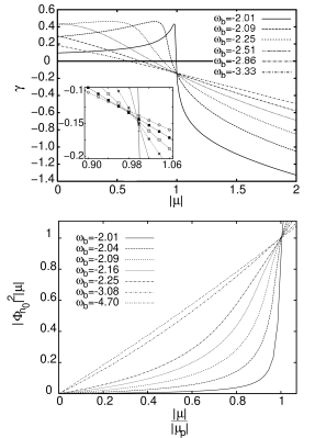
Figure 1: (a) The mismatch with the peakon shape, $\gamma$ , as a function of $|\mu|$, for discrete solitons found at different frequencies $\omega_{b}$. (Note in the inset that there is no common intersection of all the curves). (b) The soliton’s amplitude vs. $|\mu|$. The axes are rescaled to show that the amplitude of the peakon solutions (attained at $|\mu|=|\mu_{p}|$) are equal to $1/\sqrt{|\mu|}$, as predicted by the continuum approximation.

A noteworthy result, evident from Fig. 1, is the persistence of the discrete solitons beyond the peakon limit (which means continuability of the solutions to $\gamma<0$). The apparent intersection of different curves at one point in Fig1(a) is a spurious feature (see the inset in the figure): an accurate consideration shows that the curves actually intersect at close but different points. In contrast, the intersection of the curves in Fig. 1(b) indeed happens at a single point, which corresponds to the discrete solitons taking the peakon shape.

Figure 2 displays typical examples of the numerically found discrete solitons. It demonstrates that the solutions corresponding to $\gamma<0$ are cuspons, with a super-exponential shape, that do not exist in the continuum equation (4). The discrete character of the SM with the competing nonlinearities allows this new type of solution (as happens with the quasi-collapsing states in the standard DNLS equation in two dimensions quasicollapse ). Cuspon solutions continue into the region of $|\mu|>1$, where the CA yields no solitons, but, due to the sharp change of the solution with the increase of $|\mu|$, finding numerical solutions at larger values of $|\mu|$ becomes increasingly more difficult.

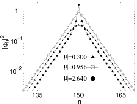
Figure 2: Generic examples of three different types of discrete solitons, for $\omega_{b}=-2.091$: a quasi-continuous $\mathrm{sech}$-like solution at $|\mu|=0.3$, a peakon at $|\mu|=0.956$, and a cuspon at $|\mu|=2.64$.

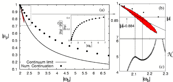
Figure 3: (Color online). (a) The value of $\left|\mu_{p}\right|$, at which the soliton assumes the peakon shape: the prediction of the continuum approximation, Eq. (10) (solid curve), and numerical results for discrete solitons (dots). Also shown is a small region where the discrete solitons are found to be unstable (for that purpose, the vertical axis shows $|\mu|$, rather than $|\mu_{p}|$). The inset displays the relative difference between the numerically found values of $|\mu_{p}|$ and the prediction, $|\mu_{p}^{CL}|$, provided by the continuum approximation. (b) Zoom of the area in the $\left(|\omega_{b}|,\left|\mu_{p}\right|\right)$ plane where the instability island is located. (c) Norm of the discrete solitons vs. the frequency, for $|\mu|=0.884$.

In Fig. 3(a) we compare the line of the existence of the peakons in the continuum limit, and the actual location of discrete peakons. It is seen that the agreement between the CA and numerical findings is good for smaller $\left|\omega_{b}\right|$ (in this case, the discrete solitons are broad), while at larger $\left|\omega_{b}\right|$ the discrete solitons are narrow, hence the agreement with the CA deteriorates.

III.1 Stability of the solitons

We have performed stability analysis of the discrete solitons by computing eigenvalues (Floquet multipliers, $\lambda_{F}$) for modes of small perturbations Floria , within the framework of the linearized equation of the SM (1). The integration of a basis of initial perturbations over a period $T_{b}$ of the discrete soliton gives the Floquet matrix that in our case is real and symplectic so that its eigenvalues come in quadruplets $\{\lambda_{F},\;1/\lambda_{F},\;\overline{\lambda}_{F},\;1/\overline{\lambda}_{F}\}$. Then, the discrete soliton solution to Eq.(1) is linearly stable if all the Floquet multipliers lie on the unit circle of the complex plane, $|\lambda_{F}|=1$. It is found that the solitons are linearly stable along the whole continuation, except for a relatively small region, as shown in Fig. 4(a). The entire instability island in the $(|\omega_{b}|,|\mu|)$ plane is displayed in Fig. 3(b). Note, in particular, that the peakon and cuspon solutions are stable. The stability of the discrete solitons was also checked by direct simulations of perturbed solitons, using the full equation (1), which corroborated the predictions of the linear analysis.

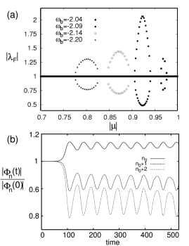
Figure 4: (a) The absolute value of the Floquet multiplier, $\left|\lambda_{F}\right|$, for the linearization of perturbations around discrete solitons, is shown vs. $|\mu|$, at several fixed values of the frequency (which are chosen so as to make the instability intervals well separated). The soliton is unstable if $\left|\lambda_{F}\right|\neq 1$. (b) A robust pulson generated from an unstable soliton at $|\mu|=0.922$.

Direct simulations of the evolution of perturbed unstable solitons, a typical example of which is displayed in Fig. 4(b), show that, after a transient stage, a localized pulson (showing simultaneous width and amplitude oscillations) is formed. The pulsons are (quasi-)periodic in time, and persist indefinitely. This behavior resembles that found in the ordinary two-dimensional DNLS equation in quasi-collapsing states quasicollapse .

A necessary stability condition for soliton families in models of the NLS type may be provided by the Vakhitov-Kolokolov (VK) criterion VK : if the norm ${\cal N}$ of the soliton is known as a function of its frequency $\omega_{b}$, the solitons can be stable against small perturbations with real eigenvalues, provided that $d{\cal N}/{d}$$\omega_{b}<0$. Although the applicability of the VK criterion to the present model has not been proven (and counter-examples are known, when solitons predicted by the criterion to be unstable are actually stable KronigPenney ), it is relevant to test the criterion here, numerically computing ${\cal N}\left(\omega_{b}\right)$ according to Eq. (2). The result is that the VK criterion precisely explains the stability and instability of the discrete solitons, except for the cuspons (see below), as shown in Fig. 3(c).

A noteworthy feature of the ${\cal N}\left(\omega_{b}\right)$ dependence is a divergence of the total norm due to the infinite contribution of the central site to expression (2) in the case of the exact peakon solution, with $\left|\Phi_{n_{0}}\right|^{2}=1/|\mu|$. An example of the ${\cal N}\left(\omega_{b}\right)$ dependence showing the divergence is plotted in Fig. 5. As concerns the cuspons, whose amplitude exceeds the critical value, $1/\sqrt{|\mu|}$, the norm (2) converges for them, and features a positive slope (see Fig. 5), $d{\cal N}/d\omega_{b}>0$. The VK criterion predicts instability in this case; however, the direct computation of the Floquet multipliers (see above), as well as direct simulations, reveal no instability of the cuspons. Thus, while the VK criterion is perfectly correct for regular solitons and peakons in the present model, it is irrelevant for cuspons, cf. the situation in Ref. KronigPenney .

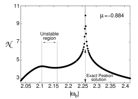
Figure 5: The norm of the discrete solitons vs. the frequency, for $|\mu|=0.884$.

III.2 Bound states of solitons and their stability

We have explored bound states of discrete solitons in Eq. (1). For this purpose, we performed numerical continuation in $\mu$, starting with the well known bound states of the standard DNLS equation, at $\mu=0$. In that limit, two different types of bound states are known, in-phase and $\pi$-out-of-phase ones, which are represented, respectively, by even and odd solutions. It is well known that only the states of the latter type are stable Todd .

The numerical continuation of soliton bound states was performed for pairs of identical discrete solitons of a given frequency $\omega_{b}$ and different distances between them. The continuation of in- and out-of-phase bound states gives bound states of peakons, see Fig. 6(a). The latter solution is found at exactly the same value, $\mu=\mu_{p}(\omega_{b})$, which gives rise to the single peakon. We have also examined the stability eigenvalues for the computed solutions. A remarkable feature of the bound states observed with increase of $|\mu|$ is the stability interchange between the in-phase and out-of-phase states, as shown in Fig. 6(b), which occurs precisely at $\mu=\mu_{p}(\omega_{b})$, regardless of the separation between the bound solitons.

(a)

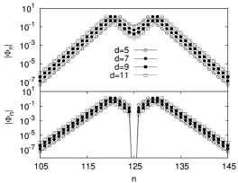
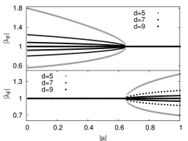
(b)

Figure 6: (a) Profiles of typical in-phase (top) and out-of-phase (bottom) bound states of two peakons, with different distances between their centers, at $\omega_{b}=-3.086$ and $|\mu|=|\mu_{p}|=0.645$ . (b) Absolute values of the Floquet multiplies that determine the stability of three bound states, with the same fixed frequency, $\omega_{b}=-3.086$, and different separations between the solitons. The in-phase (top) and out-of-phase (bottom) bound states are stabilized and destabilized, respectively, at the point where the bound solitons are peakons, see panel (a). Unstable states are less unstable (with smaller absolute values of the Floquet multipliers accounting for the instability) if the distance between the solitons is larger.

IV Moving solitons

The integrable AL model gives rise to both static and moving solitons. In the DNLS equation, moving solitons Mussl ; Papa and collisions between them Papa were also studied, using various methods. Soliton motion was also a subject of analysis in the SM, which was usually treated, in this context, as a perturbed version of the AL equation LANLcollision ; Dmitriev .

As a part of the present work, we have performed numerical continuation of mobile discrete solitons from the DNLS limit, where, in turn, they were earlier obtained by means of a continuation procedure initiated with the AL solitons MovingSolitonsDNLS . The continuation procedure is the natural extension of the one applied to static discrete solitons (i.e. based on computing fixed points of maps by means of the shooting method) and allows obtaining mobile solutions whose profiles are repeated (translated a number of sites) after an integer number of periods of the internal oscillation. These states are composed of a traveling localized core and an extended background, $\Phi_{n}=\Phi_{n}^{\mathrm{core}}+\Phi_{n}^{\mathrm{bckg}}$, see Fig. 7. The background is a superposition of nonlinear plane waves, and its amplitude is related to the height of the corresponding Peierls-Nabarro (PN) barrier, which is defined as the energy difference between two static solutions for the soliton, with a fixed frequency $\omega_{b}$, one centered at a lattice site, with $n_{0}=n$, and the other at an intersite position, with $n_{0}=n\pm 1/2$.

Figure 7: The real and imaginary parts of the lattice wave field in a moving discrete soliton, for $\omega_{b}=-2.24$ and $\mu=-0.7$.

The result obtained along these lines in the present model is that the mobile solitons can only be continued up to a certain critical value, $\mu=$ $\mu_{c}(\omega_{b})$, close to but smaller in absolute value than $\mu_{p}(\omega_{b})$, at which the static discrete soliton becomes a peakon. The Floquet stability analysis reveals that the extended background of the mobile solitons is subjected to modulational instability. (However, this is too weak to manifest itself in the simulations and it is only noticeable by looking at the Floquet spectra when the amplitude of the background is very high). On the the other hand we do not observe any localized eigenvector with eigenvalue $|\lambda_{F}|>1$ and thus the core is not affected by any unstable perturbation. The stability of mobile solutions is corroborated when simulations of the dynamics are performed allowing for interesting numerical experiments (see below). The background amplitude is a growing function of $|\mu|$ having a very sharp increase when $|\mu|$ approaches $\mu=$ $\mu_{c}(\omega_{b})$, see Fig.8(a). This behavior of the background amplitude suggests that the PN barrier also grows with $|\mu|$ and becomes very high near the critical point. To check this expectation, we have computed the height of the PN barrier for the same frequencies $\omega_{b}$ for which the mobile solitons were numerically calculated, using the energy definition as in Eq. (3). Figure 8(b) confirms that the PN barrier dramatically increases when the continuation approaches the critical point, $\mu=$ $\mu_{c}(\omega_{b})$, although the PN barrier diverges not exactly at this point, but rather at $\mu=\mu_{p}(\omega_{b})$, where the soliton assumes the peakon shape.

Figure 8: The background amplitude (a) and the height of the Peierls-Nabarro barrier (b), as functions of $|\mu|$, for three mobile discrete solitons.

The strong dependence of the PN barrier on $\mu$ suggests a numerical experiment to test the behavior of mobile solitons when the lattice’s pinning force suddenly changes. To this end, we took an initial mobile soliton at values of $\mu$ and $\omega_{b}$ for which the PN barrier is low. Then we monitored the evolution of the moving soliton following an instantaneous change in the nonlinearity, $\mu\rightarrow\mu+\delta\mu\equiv\mu^{\prime}$, which makes the PN barrier essentially higher than experienced by the original soliton. The numerical experiments are illustrated by Fig. 9. We observe that the core of the mobile lattice soliton does not become pinned due to the increase of the PN barrier, but rather accommodates itself, with some radiation loss, into a broader state with a smaller amplitude, so that the PN barrier, as experienced by the new state for $\mu=\mu^{{}^{\prime}}$, is low enough to allow the soliton to remain mobile. Besides that, we observe an increment in the core’s velocity, so that the larger the jump of the PN-barrier’s height the faster is the new moving state. The fact that the sudden increase of the PN barrier does not prevent the motion of the soliton reveals, on one hand, that the relation between PN barrier and mobility is far from trivial, and on the other hand, that mobility is quite a robust feature.

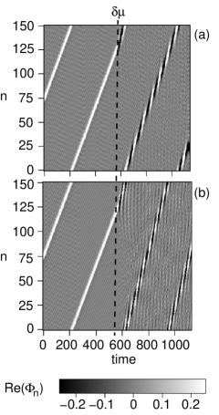
Figure 9: The time evolution of the real part of the lattice wave field in a mobile state. Initially, a moving soliton is created corresponding to $|\mu|=0.8$ and $\omega_{b}=-2.24$. Then, $\mu$ jumps instantaneously to $\mu^{\prime}=\mu+\delta\mu$. After the jump, followed by emission of some transient radiation, the moving core becomes broader and starts to move faster. In (a) $|\mu^{\prime}|=0.84$, and in (b) $|\mu^{\prime}|=0.89$.

Finally, we simulated collisions between identical lattice solitons moving in opposite directions. The results show that the colliding solitons always merge into a single localized state, which subsequently features intrinsic pulsations. If the PN barrier is low, the emerging pulse can itself move in a chaotic way, due to interaction with the lattice phonon field (radiation) generated in the course of the collision. On the contrary, for values of $\mu$ and $\omega_{b}$ at which the original solitons experience a high PN barrier, the finally generated single soliton is always strongly pinned.

The most notable and generic feature of the collision manifests itself in the merger scenario. When the cores of the mobile solitons collide, sudden delocalization is first observed, with transfer of energy from the collision point to adjacent lattice sites. Then, almost all the energy is collected back at the collision spot, and thus a single localized state emerges. An example of the collision is shown in Fig. 10. This scenario was observed in all simulations of the collisions. The appearance of pulsons as the product of soliton collisions, as well as the fact that they also appear as asymptotic states of the evolution of perturbed unstable solitons (see Section III.1), shows the ubiquity of this type of localized excitations in the present model.

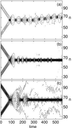
Figure 10: Contour plots showing the evolution of the lattice field $|\Phi_{n}|$ in three cases of collisions between identical solitons moving in opposite directions. The soliton’s frequency is $\omega_{b}=-2.11$, and $|\mu|=0.6$ (a), $|\mu|=0.8$ (b), and $|\mu|=0.9$ (c).

V Conclusion

We have introduced a combination of the DNLS and Ablowitz-Ladik models with competing nonlinearities (self-focusing onsite and self-defocusing intersite cubic terms). The model may describe a condensate of bosonic dipoles trapped in a strong lattice potential. First, it was shown that the continuum counterpart of the model gives rise to solitons in a finite band of frequencies, with broad, small-amplitude NLS-like solitons at one edge of the band, and an exact solution in the form of a peakon at the other. Numerical analysis of the discrete system yields a similar family of solitons, which also includes a peakon; however, the family continues beyond the peakon, in the form of discrete cuspons. Stability of the lattice solitons was investigated by means of the computation of their Floquet spectra, and in direct simulations. It was found that only a small part of the soliton family is unstable; the evolution of the unstable solitons leads asymptotically to pulsons, i.e. localized solutions where the width oscillates. In particular, peakons and cuspons are stable. Additionally, it was found that the Vakhitov-Kolokolov criterion precisely explains the stability and instability of regular solitons, but does not apply to cuspons, for which it erroneously predicts instability. Bound states of identical solitons were also investigated, revealing a stability exchange: the in-phase and out-of-phase bound states, which are unstable and stable, respectively, in the DNLS limit, exchange their stability character exactly at the point where the bound solitons are peakons.

We have numerically computed mobile solitons with the same high precision as for the static ones. Their structure is that of an exponentially localized core on top of an extended background (which is a superposition of a finite number of extended plane waves). The amplitude of the background is correlated with the height of the computed Peierls-Nabarro barrier. The mobile solitons exist up to a critical value of the strength of the self-defocusing intersite nonlinearity, which is lower than (but close to) the corresponding value for which the peakon state exist. Collisions between solitons always lead to their merger into a pulson state.

References

- (1) M. Johansson, S. Aubry, Y. B. Gaididei, P. L. Christiansen, and K. Ø. Rasmussen, Physica D 119, 115 (1998); P. G. Kevrekidis, K. Ø. Rasmussen, and A. R. Bishop, Int. J. Mod. Phys. B 15, 2833 (2001).
- (2) M. J. Ablowitz and J. F. Ladik, J. Math. Phys. 17, 1011 (1976).
- (3) B. A. Malomed and M. I. Weinstein, Phys. Lett. 220, 91 (1996).
- (4) M. Salerno, Phys. Rev. A 46, 6856 (1992); see also Encyclopedia of Nonlinear Science, p. 819 (ed. by A. Scott, New York, Routledge, 2005).
- (5) D. Cai, A. R. Bishop, and N. Grønbech-Jensen, Phys. Rev. E 53, 4131 (1996); K. Ø. Rasmussen, D. Cai, A. R. Bishop, and N. Grønbech-Jensen, ibid. 55, 6151 (1997).
- (6) D. Cai, A. R. Bishop, and N. Grønbech-Jensen, Phys. Rev. E 56, 7246 (1997).
- (7) S. V. Dmitriev, P. G. Kevrekidis, B. A. Malomed, and D. J. Frantzeskakis, Phys. Rev. E 68, 056603 (2003).
- (8) J. Gómez-Gardeñes, F. Falo, and L.M. Floría, Phys. Lett. A 332, 213 (2004); J. Gómez-Gardeñes, L.M. Floría, M. Peyrard, and A. R. Bishop, Chaos 14, 1130 (2004).
- (9) Z. D. Li, P. B. He, L. Li, J. Q. Liang, and W. M. Liu, Phys. Rev. A 71, 053611 (2005).
- (10) Kh. I. Pushkarov, D. I. Pushkarov, and I. V. Tomov, Opt. Quant. Electr. 11, 471 (1979); S. Cowan, R. H. Enns, S. S. Rangnekar, and S. S. Sanghera, Canad. J. Phys. 64, 311 (1986).
- (11) Discrete solitons are also widely referred to as discrete breathers because of the ocillatory dynamics of the real and imaginary part of the complex variables .
- (12) J.L. Marín, and S. Aubry, Nonlinearity 9, 1501 (1996).
- (13) T. Cretegny, and S. Aubry, Phys. Rev. B 55, R11929 (1997).
- (14) E. W. Laedke , K. H. Spatschek, and S. K. Turitsyn, Phys. Rev. Lett. 73, 1055 (1994).
- (15) J.L. Marín, S. Aubry, and L.M. Floría, Physica D 113, 283 (1998).
- (16) M. G. Vakhitov and A. A. Kolokolov, Sov. J. Radiophys. Quant. Electr. 16, 783 (1973); see also a review: L. Bergé, Phys. Rep. 303, 260 (1998).
- (17) I. M. Merhasin, B.V. Gisin, R. Driben, and B.A. Malomed, Phys. Rev. E 71, 016613 (2005).
- (18) T. Kapitula, P. G. Kevrekidis, and B. A. Malomed, Phys. Rev. E 63, 036604 (2001); D. E. Pelinovsky, P. G. Kevrekidis and D. J. Frantzeskakis, Physica D 212, 1 (2005).
- (19) M. J. Ablowitz, Z. H. Musslimani, and G. Biondini, Phys. Rev. E 65, 026602 (2002).
- (20) I. E. Papacharalampous, P. G. Kevrekidis, B. A. Malomed, and D. J. Frantzeskakis, Phys. Rev. E 68, 046604 (2003).