Synchronization on fast and slow dynamics in drive-response systems

Abstract

Two types of synchronization, Achronal Synchronization and Isochronous synchronization are investigated numerically when unidirectionally coupled laser systems are considered both on fast and slow dynamics by studying the correlation function. Although the synchronization behaviors are found to be separated on relatively fast dynamics of chaotic fluctuations while blended together on slow dynamics of dropout events, their main features revealed are in a good agreement, which most probably suggests that the observation based on detections on slow dynamics is of importance when it is the only choice as detection on fast dynamics is usually extremely hard to be done.

I Introduction

Synchronization between coupled chaotic oscillators is a fundamental phenomenon widely observed in science and naturePecora and Carroll (1990). It has various applications, especially in secure communication where it can be used to enhance the privacyVanWiggeren and Roy (1998). For two coupled identical oscillators, Complete Synchronization (CS) may occur between themTang and Liu (2003); Masoller (2001); Ahlers et al. (1998); Liu et al. (2001). However there are often correlated entrainments of discrete events when nonidentical ones are considered, meanwhile their fast chaotic behaviors remain asynchronous, which is often referred to as phase synchronization (PS) phenomenonRosenblum et al. (1996, 1997); Ivanchenko et al. (2004a). Typical examples are: (i)neuronal system may produce common rhythmic bursting as there is coupling between neurons, while its individual neurons still show asynchronous dynamics of fast spikingElson et al. (1998); Rulkov (2001); Dhamala et al. (2004); Ivanchenko et al. (2004b); (ii)coupled semiconductor lasers operating in low frequency fluctuation (LFF) may produce rhythmic dropout events whereas their fast chaotic dynamics remain largely differentWallace et al. (2001); Wedekind and Parlitz (2002); Buldú et al. (2002); Heil et al. (2001); Sivaprakasam et al. (2001). On the other hand, the existing coupling would still introduces some correlation between the involved oscillators in spite that their dynamics are seemly completely asynchronous. It is possible that there is certain functional relations between their outputs, a situation which is often called generalized synchronization (GS)Rulkov et al. (1995); Kocarev and Parlitz (1996), while those explicit functions prove to be difficultly recognized in many other cases, the still existing correlation would show itself by some similarities function, such as correlation function, mutual information function and so on.Rosenblum et al. (1997)

Although a large number of papers about synchronization have been published in which both fast and slow dynamics are concernedHramov and Koronovskii (2004); Dhamala et al. (2004); Ivanchenko et al. (2004b); Elson et al. (1998), unfortunately little work has been done in such framework on Achronal and Isochronous synchronization which are simultaneously existing ubiquitously in most drive-response systems.

This two qualitatively different types of synchronization, Isochronous and Achronal synchronizationLocquet et al. (2002a); Koryukin and Mandel (2002); Murakami and Ohtsubo (2002); Locquet et al. (2002b); Uchida et al. (2004); Voss (2000), are discussed in this paper when both fast and slow dynamics are concerned. On one hand the directed coupling from one laser to another may be strong enough to lead to a locking state phenomenon and consequently Isochronous Synchronization (IS). On the other hand, Achronal Synchronization (AS) may also occur, corresponding to the mathematical solution of equations describing the subsystems’ behaviors. We show that the synchronization behaviors are clearly separated on fast dynamics, while blended together on slow dynamics. Moreover most important features about synchronization can be well reflected by both fast and slow dynamics, which most probably suggests the observation on slow dynamics is of importance when it is the only choice as detection on fast chaotic dynamics is usually technically hard to be done.

II Synchronization States

The following equations are used to describe a typical drive-response (directed coupled) system:

$$\dot{X}_{t}=f(X_{t},\gamma X_{t-\tau})$$ (1)

$$\dot{Y}_{t}=f(Y_{t},\eta_{12}X_{t-\tau_{12}})$$ (2)

where $\gamma$ represents the feedback rate in drive-subsystem(X), $\eta_{12}$ is the coupling strength from drive-subsystem(X) to response-subsystem(Y). $\tau$ is the delay involved in feedback, and $\tau_{12}$ corresponds to the retardation time for the coupling from X to Y. Two basic types of synchronization probably occurring in such systems are:

$$Isochronous\ Synchronization : Y_{t}\sim X_{t-\tau_{12}}$$ (3)

$$Achronal\ Synchronization : Y_{t}\sim X_{t+(\tau-\tau_{12})}$$ (4)

For the reason that synchronization is a universal nonlinear phenomenon, and its main features are typically independent of particular properties of a model, a system consisting of two semiconductor lasers in drive-response configuration as an example is considered in this paper. One laser acts as the drive-subsystem (called Master) and it is driven into low-frequency-fluctuation (LFF) operating regime by being subjected to a feedback introduced by a mirror. In addition, a part of its output is injected into another laser acting as the response-subsystem (called Slave). This injection drives the Slave laser into LFF regime as well as introduces a coupling directed from Master to Slave. The two lasers’ behaviors can be described and numerically simulated by LK modelLang and Kobayashi (1980).

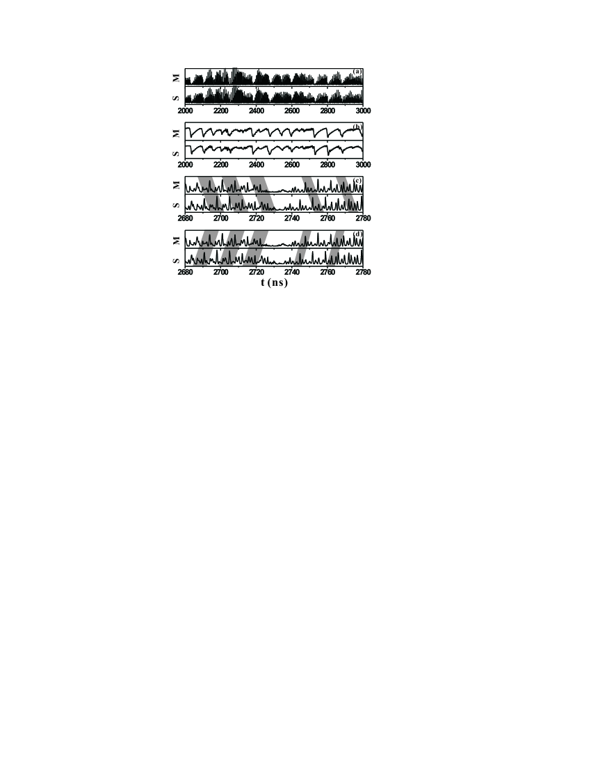
Figure 1: Outputs of two unidirectionally coupled semiconductor lasers simulated by LK model. chaotic low-frequency-fluctuation behaviors of two correlated lasers from 2000-3000 nanosecond in (a), M presenting Master laser and S Slave laser. Their corresponding low-pass-filtered time series in (b) where dropout events are highlighted to show the correlation on slow dynamics. a relatively short period of time series, emphasizing Isochronous synchronization in (c) and Achronal synchronization in (d) on fast dynamics.

It is found numerically that synchronization phenomenon is occurring on both fast and slow dynamics. Fig. 1(a) plots chaotic outputs of Master and Slave lasers both operating in low-frequency-fluctuation regime from 2000 nanosecond to 3000 nanosecond where it is seen dropout events taking place rhythmically in two lasers. Those dropouts are further highlighted in Fig. 1(b) where the low-pass-filtered time series are plotted and where it is clearly seen there is Phase Synchronization occurring on slow dynamics in a timescale of dropout events shown by the easily observable rhythm between the outputs. On the other hand, a relatively short period of time series ranging from 2680 nanosecond to 2780 nanosecond are shown in Fig. 1(c) as well as in Fig. 1(d). Some gray parallelograms are added in the plots to make it clear the similarities between the detailed chaotic outputs of Master and Slave. The continuously existing similarity relationship between the lasers’ outputs in shadowed as well as unshadowed areas lasting for a relatively long period of time together lead to the emergence of the synchronization on fast dynamics in a time scale of seemly random fluctuations.

We notice the delay in feedback is set $\tau=7ns$ in our calculation, and the coupling retardation time $\tau_{12}=4ns$. Focus has been put upon Isochronous Synchronization in Fig. 1(c) where the output of Master laser is ahead of that of Slave laser by around 4 nanoseconds, satisfying Eq. (3); while Fig. 1(d) stresses Achronal Synchronization with the output of Master laser lagging behind that of the Slave laser by about 3 nanoseconds, satisfying Eq. (4), although the same piece of time series is presented in Fig. 1(3) and (4). Therefore the two types of synchronization behaviors are simultaneously occurring .

III Comparison between Fast and Slow Dynamics

The qualities of synchronization behaviors are usually measured by correlation function as a function of the shift time ($\tau_{s}$).

$$C(\tau_{s})=\frac{\langle[I_{m}(t+\tau_{s})-\langle I_{m}\rangle][I_{s}(t)-\langle I_{s}\rangle]\rangle}{\{\langle[I_{m}(t)-\langle I_{m}\rangle]^{2}\rangle\langle[I_{s}(t)-\langle I_{s}\rangle]^{2}\rangle\}^{1/2}}$$ (5)

Complete synchronization should be indicated by $C=1$, and higher correlation implying a better synchronization. On the other hand, poor synchronization would give a relatively low correlation C and hence a low synchronization quality.

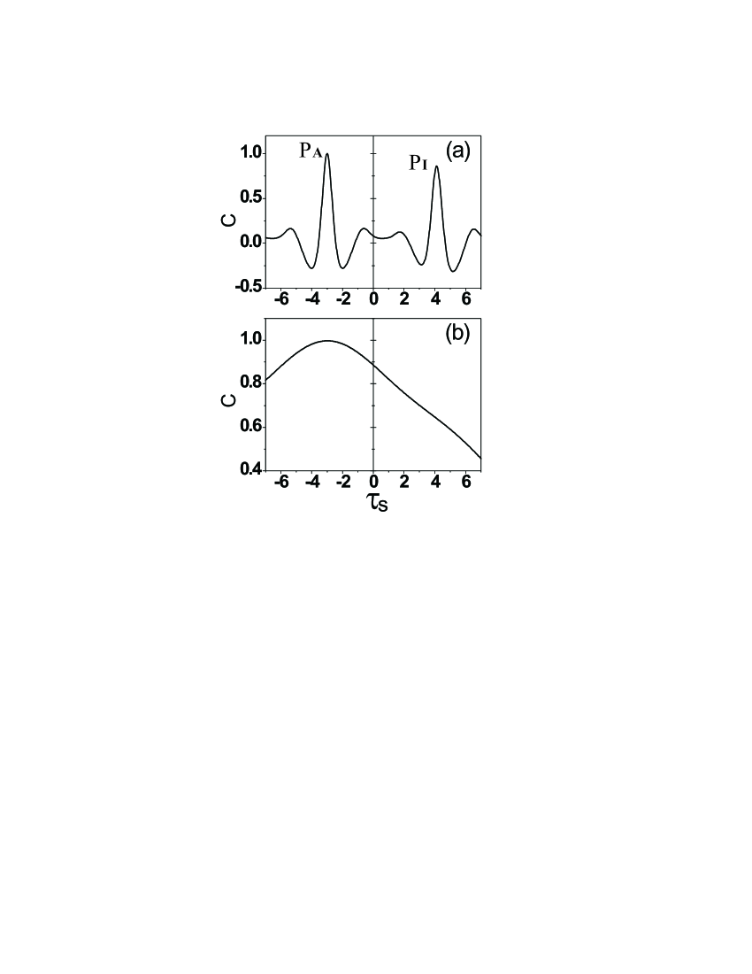
Figure 2: Correlation plots calculated (a) by original time series to reflect synchronization behaviors on fast dynamics, (b) by low-pass-filtered time series to show on slow dynamics. $\gamma=\eta_{12}=7ns^{-1}$

Fig. 2 quantitatively presents the synchronization quality of the two synchronization behaviors. Correlation function plotted in Fig. 2(a) is calculated by original time series in order to show the features on fast chaos, meanwhile correlation function by calculating on low-pass-filtered series is plotted in Fig. 2(b) to show the features on slow dynamics. There are two peaks emerging in Fig. 2(a), One ($P_{A}$) corresponds to Achronal synchronization and the other($P_{I}$) to Isochronous Synchronization ($P_{I}$). The peak at $\tau_{s}=4ns^{-1}$ indicates that a high correlation would be obtained when the output of Slave laser is shifted forward by 4ns with respect to that of Master laser and satisfying Eq. (3) and hence corresponds to Isochronous Synchronization. $P_{I}$ represents the peak value. On the other hand, the peak at $\tau_{s}=-3ns^{-1}$ shows the high correlation obtained when shifted backward by 3ns and satisfies Eq. (4), therefore Achronal Synchronization is revealed in this way with its corresponding peak value $P_{A}$. In contrast, there is only a hump in Fig. 2(b), which comes from the fact that the two synchronization behaviors are blended with each other on slow dynamics.

By comparing the correlation function of fast dynamics in Fig. 2(a) with that of slow dynamics in Fig. 2(b), their difference can be clearly seen: firstly, the very steep slope on both sides of the two peaks in Fig. 2(a) prove that the shift time of the correlation peaks are considerably explicit, $-(\tau-\tau_{12})$ for Achronal Synchronization and $\tau_{12}$ for Isochronous Synchronization, which most probably indicates that the two peaks as well as the corresponding synchronization behaviors they represent are completely separate and uncorrelated on fast dynamics. In contrast, gentler declination of the correlation from the hump in Fig. 2(b) with $C_{(\tau_{s}=0)}=0.88$ much greater than that in Fig. 2(a) suggests that Achronal and Isochronous synchronization behaviors are entangled and can not be separated from each other. As a result, they show themselves by probability distribution and consequently there is only a hump. Secondly, the two synchronization behaviors compete with each other. The competition result is reflected by the comparison which correlation peak is higher on fast dynamics on fast dynamics, while on slow dynamics the hump is clearly tilted towards one side, indicating the synchronization behavior corresponding to this side is more probably selected over the other by the system.

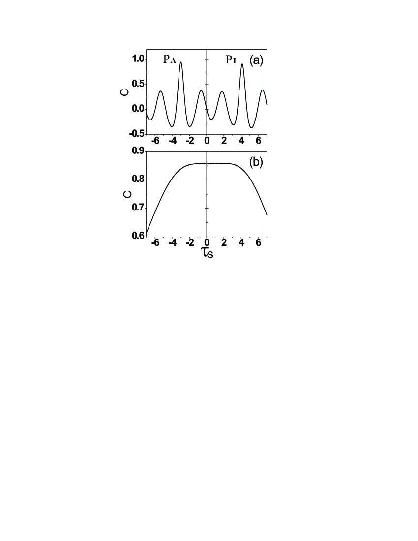
Figure 3: The balance in quality between the two synchronization behaviors on fast and slow dynamics.

Moreover, such blend of the two synchronization behaviors on slow dynamics will come to its highest level when they are balanced in quality under a very special condition. In Fig. 3(a) the nearly equi-altitude correlation peaks on two sides shows the balance in quality of the behaviors on fast dynamics, on the other hand the two peaks surprisingly turn into a single correlation plateau when slow dynamics are concerned in Fig. 3(b). It is seen $C_{(\tau_{s}=-3)}=C_{(\tau_{s}=0)}=C_{(\tau_{s}=4)}$ on this plateau, which indicates the hump as shown in Fig. 2(b) would tilt to neither side, namely neither of the synchronization behaviors are selected by the system over the other. The correlation peaks therefore disappear completely, reaching a so-called ”free state” in which there is no certain value of $\tau_{s}$ by which time series are shifted to be able to ensure a greater correlation.

Fast and slow dynamics are both capable of showing the main dynamical features of the occurring synchronization. The following part will focus on the correspondence between them. Fig. 4 shows how the result of their competition depends on the coupling strength. Here the competition result means which one of the two synchronization behaviors will be more probably selected by the system over the other. For fast dynamics the result can be shown by $P_{I}-P_{A}$, the difference between the two correaltion peak-values, see Fig. 4(a). A larger $P_{I}-P_{A}$ indicates that Isochronous Synchronization is more probably selected over Achronal synchronization, and the system’s dynamical behavior, as a result, is mainly governed by the former. Such domination can be clearly shown as well by the fact that the similarities in Fig. 1(c) emphasizing Isochronous Synchronization would have been more recognizable and easily seen than those in Fig. 1(d) which emphasize Achronal synchronization. In contrary, a minus value of $P_{I}-P_{A}$ would indicate Achronal Synchronization is the one ruling synchronization behavior of the system .

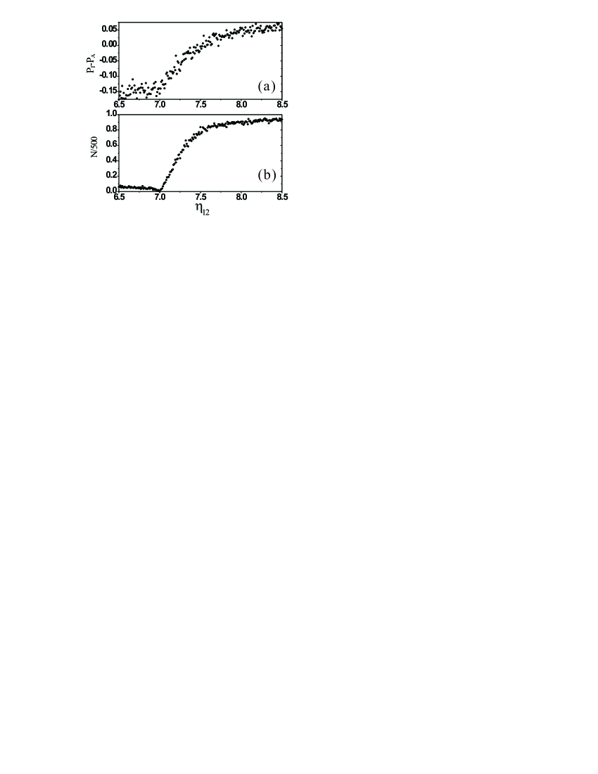
Figure 4: Competition result between the synchronization behaviors, shown on fast dynamics by $P_{I}-P_{A}$ and on slow dynamics by $N/500$, depending on the coupling strength $\eta_{12}$.

As for slow dynamics, a quantity $N/500$ is able to measure the competition result by showing the probability that the dropouts in Master laser are ahead of the corresponding ones in Slave laser. In the calculation of $N/500$, 500 dropout pairs are identified firstly by the condition that two dropouts from different lasers are paired when they are close to each other with the time interval less than 8 nanoseconds, subsequently they are judged one by one which laser’s output is ahead in time. Finally the value of N shown in Fig. 4(b) is obtained by counting the number of those dropout pairs in which Master’s dropout occurs ahead of Slave’s in time. The closer $N/500$ is to 1, the more probably Isochronous Synchronization is selected by the system over Achronal synchronization, in contrary $N/500<0.5$ means Achronal Synchronization is more probably selected. Since not outputs in detail but just the dropout events are concerned in $N/500$, Fig. 4(b) considers the features on slow dynamics.

In Fig. 4 both $P_{I}-P_{A}$ and $N/500$ are seen to increase gradually in the region from 7.0 to 7.6 ns^-1, suggesting that the role of ruling system synchronization behavior has been transferred from Achronal to Isochronous Synchronization. The transition process slows down when coupling strength is greater than 7.6 ns^-1 in both figures. Therefore there is a good agreement between fast and slow dynamics. The coupling is too weak to produce continuous synchronous behavior both on fast and slow dynamics when $\eta_{12}<7.0$.

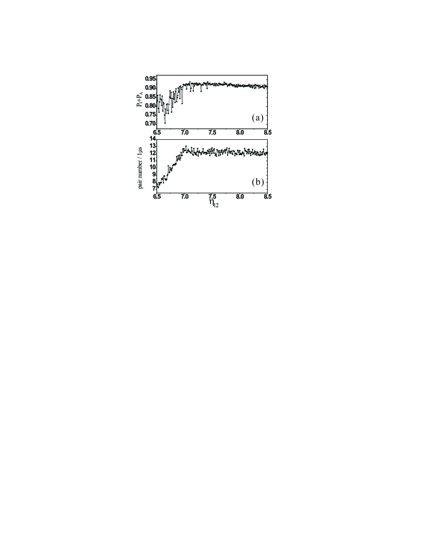
Figure 5: The overall synchronization quality, shown on fast dynamics by $P_{I}+P_{A}$ and on slow dynamics by the averaged number of dropout pairs every microsecond, depending on the coupling strength.

That the features of synchronization behaviors can be shown by both fast and slow dynamics is further shown in Fig. 5, where the dependence of $P_{I}+P_{A}$ (a) and the number of dropout pairs per microsecond (b) on the coupling strength $\eta_{12}$ is plotted. Since on fast chaos the two synchronization behaviors are shown by two separated correlation peaks with the peak-values $P_{I}$ and $P_{A}$ and they take place simultaneously, the summation of $P_{I}$ and $P_{A}$ seems useful to estimate the overall synchronization quality. From $\eta_{12}=6.5$ to 7.0ns^-1, $P_{I}+P_{A}$ has being increased before it comes to its maximum value $\eta_{12}=7.0ns^{-1}$ around which the overall synchronization quality, when $\eta_{12}$ is over 7.0ns^-1, remains almost unchanged. These changing procedures are capable of being reflected by slow dynamics as well. In average there are about 12.5 dropouts per microsecond generated in each laser. However some dropouts of Master laser are not capable of being connected with dropouts from Slave laser to form dropout pairs when the coupling is not sufficiently strong. It is expected when the coupling is enhanced that the resulting correlation is strengthened and that the forming-pair rate rises steadily till to its extreme level so that all of the dropouts can find their partners from the other laser to form pairs with the number of pairs per microsecond remaining around 12.5 pairs per microsecond. Through the comparison Fig. 5(a) with Fig. 5(b), it is obvious that fast and slow dynamics are in a good agreement when they are used to study the dynamical features of the occurring synchronization.

IV Discussion

Both Fig. 4(a) and (b) show the fact that the improvement of overall synchronization quality to its full level is a gradual course. That is to say, the transition of system behavior from asynchrony to synchrony is not a sudden change, but a progressive one where the overall synchronization quality is improved little by little.

The correspondence between fast and slow dynamics is shown not only when the overall synchronization has been fully established, i.e. $\eta_{12}>7.0$, but also in the region where it has not yet when $\eta_{12}<7.0$. For example, Achronal and Isochronous synchronization are both improved steadily with the increase of the coupling coupling strength and the former is always better than the later when $\eta_{12}$ is less than 7.0ns^-1. These things can be reflected by the fact that $P_{I}$ is always less than $P_{A}$ in Fig. 4(a) regarding fast dynamics, and that $N/500$ remains less than 0.1 and almost unchanged in Fig. 4(b) regarding slow dynamics.

V Conclusion

This paper compares the dynamical features of the synchronization behaviors revealed by fast dynamics with those revealed by slow dynamics. Although there are differences especially in the way the synchronization behaviors are shown, most other important features about synchronization reflected by fast and slow dynamics are in agreement, which most probably suggests that the observation based on the detection on slow dynamics is of importance when it is the only choice as detection on fast dynamics is technically hard to be done experimentally.