Quantitative laboratory observations of internal wave reflection on ascending slopes

Abstract

Internal waves propagate obliquely through a stratified fluid with an angle that is fixed with respect to gravity. Upon reflection on a sloping bed, striking phenomena are expected to occur close to the slope. We present here laboratory observations at moderately large Reynolds number. A particle image velocimetry (PIV) technique is used to provide time resolved velocity fields in large volumes. The generation of the second and third harmonic frequencies are clearly demonstrated in the impact zone. The mechanism for nonlinear wavelength selection is also discussed. Evanescent waves with frequency larger than the Brunt-Väisälä frequency are detected and experimental results agree very well with theoretical predictions. The amplitude of the different harmonics after reflection are also obtained. Keywords: Stratified fluids – Internal waves – Nonlinear Physics PACS numbers: 47.55.Hd Stratified flows. 47.35.+i Hydrodynamic waves.

I Introduction

The oblique propagation of internal waves follows from the dispersion relation that monochromatic perturbations of frequency $\omega$ have to satisfy

$$\omega=\pm N\sin\theta,$$ (1)

where $N$ is the Brunt-Väisälä frequency

$$N=\sqrt{-\frac{g}{\rho_{0}}\frac{\partial\rho}{\partial z}},$$ (2)

$g$ being the gravity, $\rho(z)$ the ambient density profile and $\rho_{0}$ a reference density. This dispersion relation shows that for a fixed frequency, the direction in which energy propagates with respect to the horizontal, $\theta$, is fixed. Moreover, Eq. (1) determines that phase and energy propagate in perpendicular directions. For set-up with Brunt-Väisälä frequency $N$ independent of $z$, observations of internal waves have invariably showed [15, 2] this transverse and oblique propagation.

The above dispersion relation is obtained, away from any turbulent portions of the domain, by substituting a plane wave $A\exp[ik(x\sin\theta+z\cos\theta)]$ of wavenumber $k$ and amplitude $A$ in the wave equation governing the horizontal velocity $u$

$$u_{ttxx}+u_{ttzz}=-N^{2}u_{xx},$$ (3)

where subscripts denote partial derivative, $x$ and $z$ refer to Cartesian coordinates and $t$ to time. The vertical velocity $w$, the perturbation pressure $p$, the streamfunction $\psi$ and the perturbation density satisfy the same hyperbolic equation (3).

The presence of a solid horizontal bottom, a free surface or an oblique slope results in a reflected wave with the same intrinsic wave frequency as the incident one. Linear internal wave reflection on a sloping bottom has been treated analytically by different authors [18, 4, 23]. The striking consequence of the geometric focusing of linear internal waves has also been reported [13, 12, 11]. Under appropriate conditions, it leads to internal wave attractors in confined stably stratified fluids. For critically incident waves for which the slope and energy propagation angles coincide, the linear inviscid analysis becomes singular and an infinite amplitude of the reflected wave was predicted [18].

Experiments on internal wave reflection were first performed by Cacchione and Wunsch [1] using conductivity probe measurements. A tidal-like excitation was generated in a 5 m long tank by a horizontally oscillating paddle; the incident and reflected waves from a $15^{\circ}$ slope were separated using periodogram estimates to compute wave amplitude and wavenumber. Although these pioneering results were of poor quality (compared to what is possible nowadays), their shadowgraph experiments showed nevertheless striking microstructures along the slope, reminiscent of an array of vortices along the slope’s boundary layer. Thorpe and Haines [24] measured dye band displacements on a $20^{\circ}$ slope providing qualitative agreement with linear theory and also noticed three dimensional boundary layer structures. Subsequently, Ivey and Nokes [7] estimated the mixing efficiency above a $30^{\circ}$ slope submitted to modal excitation and visualized with rainbow Schlieren technique: the weakening of the background stratification was measured and the corresponding change in potential energy compared to the mechanical work provided by the wave-maker. The internal wave reflection mechanism has also been studied in close connection with its importance for the creation of nepholoid layers by McPhee and Kunze [14]. More recently, Dauxois, Didier and Falcon [2] performed Schlieren experiments on critical reflection, focusing on the boundary layer upwelling events and providing good qualitative agreement with the previous weakly nonlinear study [3]. Finally, using synthetic Schlieren measurements, Peacock and Tabaei [17] showed the second harmonic generation. To our knowledge, no local quantitative amplitude measurements of internal wave reflection have been so far performed.

Recently, the weakly nonlinear theoretical issue has been put forward. It has been shown by Dauxois and Young [3] that the singularity can be healed using matched asymptotic expansion. Their analysis describes the build up of the reflected wave along the slope for a incident plane wave. Always from the theoretical point of view, the reflection of internal waves was revisited by Tabaei, Akylas and Lamb [21] for the case of a narrow incident beam but for non-critical angles. In this case, they have predicted the generation of harmonics in the steady regime; this result has not been addressed experimentally yet. Besides, fully nonlinear numerical simulations have also been performed to examine the behavior of large-amplitude internal gravity waves impinging on a slope [19, 9, 20, 10, 25].

Here we present the results of laboratory experiments in which a beam of internal waves is reflected on an oblique slope. Experiments were carried out in the 13m diameter Coriolis platform, in Grenoble, filled with salted water. The large scale of the facility allows us to strongly reduce the viscous dissipation along wave propagation and, moreover, quantitative results are obtained thanks to high resolution Particle Image Velocimetry (PIV) measurements.

The paper is organized as follows. In Sec. II, we present the experimental set up and discuss all control parameters. In Sec. III, we show the experimental results. We explain in Sec. III.1 the spectral analysis used to distinguish the different harmonics. In the following section III.2, we discuss the mechanism of wavelength selection. Section III.3 is devoted to the evanescent waves, while Sec. III.4 discuss amplitude measurements. Section IV concludes and gives some perspectives.

II Experiments

II.1 Experimental setup

We developed an original internal wave exciter inspired by Ivey et al. [8] in order to produce a two and a half wavelengths beam. A PVC sheet was compressed on both sides by seven squared arms (Fig. 1) fixed on a long central axis via eccentric wheels. The axis was set in rotation by a stepping motor, generating a longitudinal oscillation motion of 8 cm amplitude along the 60 cm width of the paddle. The frequency of excitation, proportional to the angular speed of the motor could be precisely monitored in order to vary the angle of propagation of internal waves. The wavelength was also varied from 11.3 to 12.6 cm. The paddle itself was inclined at an angle $\Phi=13^{\circ}$ with the horizontal to increase excitation efficiency. If the main part of the energy is indeed transmitted to a beam of internal wave of frequency $\omega$, higher harmonics $n\omega$ are also excited by the oscillating paddle. Nevertheless, as their frequencies are higher, their propagation angles are also larger. Taking advantage of this fact, a screen has been appropriately located above the bottom-end of the glass plate so that all harmonics are reflected to the left, and do not perturb the region of interest. The emitted plane wave hits a $2\times 3$ meters glass plane (see Fig. 1) , back-painted in black to avoid parasite laser beam reflections.

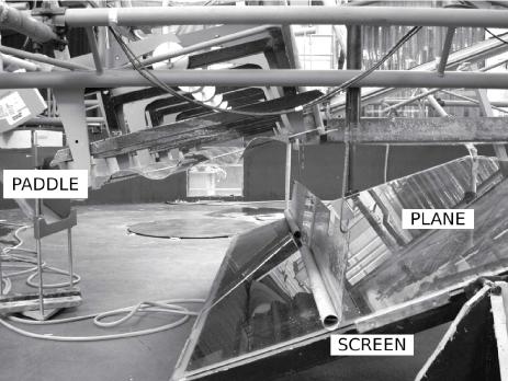
Figure 1: Picture of the experimental setup. The 3 meters long oscillating paddle generates incident internal waves which are impinging on the inclined glass plane visible on the left. One also clearly sees the screen which avoids the propagation toward the glass plane of harmonics also generated by the paddle. This picture was taken before the 13 m diameter tank has been filled with 1 m of stratified salt water.

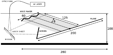
Figure 2: Sketch of the vertical cross-section of the experimental setup. The sinusoidal thick line on the top left indicates the position of the oscillating paddle, while the grey region defines the incident beam impinging on the sloping glass plane. The optic fibre, indicated by the solid line on the left, shines a laser light which is reflected on the underwater 45 degree mirror, making a thin vertical laser sheet necessary for the PIV measurements. Finally, the dashed line shows the position of the screen which avoids the propagation toward the glass plate of harmonics also generated by the paddle. A slit in the screen allows the laser sheet to pass through. All distances are in centimeter.

The above experimental set up was put in the 13 m diameter Coriolis tank filled from below with salt water and stratified by computer controlled volumetric pumps from two 75 m³ tanks, one filled with salt water and the other one with pure water. A fast conductivity probe and a temperature probe were lowered slowly into the tank using a controlled vertical micro-stepping motor to measure the stratification. The density probe was calibrated using an Anton Paar densitometer accurate to 0.0001 kg/m³ and 0.01^∘C. The linearity of the resulting density gradient was of very good accuracy, and only the upper 5 cm and the bottom 10 cm were not linearly stratified. Observations have thus been performed in the intermediate region where the Brunt-Väisälä frequency is a very well defined constant.

The stratification of 2.2% over the 1 meter depth of the tank led to a Brunt-Väisälä period $2\pi N^{-1}=13.6$s. All experiments we discussed were performed without rotation of the tank, and thus involve pure internal waves.

We used the Particle Image Velocimetry (PIV) facility of the Coriolis Platform to obtain top and side views of the velocity field. The fluid was seeded with 400 microns diameter particles polystyrene beads that were carefully prepared by a process of cooking which decreases slightly the density and successive density separations. One thus obtains a flat distribution of densities matching that of the salt stratification. This process ensures that there are equal number densities of particles at each depth. A surfactant was added to prevent the polystyrene beads from clustering. It has been shown that the relaxation time for particles to attain velocity equilibrium [16] is about 0.02s which is much shorter than the characteristic time scale of the flow. As usual, the particles are considered as passive tracers of the fluid motion.

With this method, motion is vizualized by illuminating particles with a laser sheet, which are followed by a digital camera. The laser is intentionally kept out of focus (approximately 1 cm sheet width), enabling tracking of particles despite some cross sheet displacement. Velocity fields within the plane of the laser sheet are obtained by comparing patterns in two subsequent image frames (taken 1 s apart).

The 6 Watt green Argon laser was placed above the free surface, but the light was reflected on a 45 degree mirror placed in the water (see Fig. 2). Thanks to a second underwater 45 degree mirror, the images were acquired by a 1024*1024 pixels CCD camera also located above the free surface. The cross-correlation PIV algorithm designed by Fincham and Delerce [5] was used to convert the images into vector fields (stored in the standard file format NetCDF). This algorithm provides good anti-aliasing and peak-locking rejection procedures. Our resolution went to subpixels distortions, corresponding to submillimetric displacements of the fluid. Typical maximal displacement in an image pair corresponds to 5 pixels, with a measurement precision of 0.2 pixel for an individual field (4$\%$ relative precision). This is mostly a random error, so the precision on averaged fields is higher. Finally, the analysis of the .nc files was performed with Matlab software.

Typical experimental runs lasted about 20 minutes. The first 10 periods were considered as an initial transient. Data were thus only recorded throughout the second stage during which the steady regime was attained.

II.2 Characteristics of the incident wave beam

The set of chosen excitation periods (see Table 1) leads through the dispersion relation (1) to different angles of propagation $\theta$ ranging from 13 to $25^{\circ}$. As the slope angle $\alpha$ is set to 22^∘, these cases allow us to analyze subcritical ($\theta<\alpha$), supercritical ($\theta>\alpha$) or critical ($\theta\simeq\alpha$) reflections. Finally, as the wavemaker is slightly tilted ($13^{\circ}$) from the horizontal, one has to take into account that the wavelength slightly varied from one run to another, around a typical value of $\lambda_{0}=12$ cm.

Run	1	2	3	4	5
$T$ (s)	60	49	41.5	36	32
$\theta$ (deg.)	13	16	19	22	25
$\alpha$ (deg.)	22	22	22	22	22
$\lambda$ (cm)	11.3	11.7	12.0	12.2	12.6
$u_{max}$ (cm/s)	0.412	0.566	0.775	1.000	1.225

Table 1: Summary of experimental runs with all control parameters. $T$ is the excitation period, $\theta$ the angle of energy propagation, $\alpha$ the angle of the slope defined in Fig. 3 and $\lambda$ the wavelength of the incident beam. $u_{max}$ is the maximum horizontal velocity that has been measured.

Previous experimental studies of internal wave reflection have reported the importance of viscous dissipation [2, 17, 6] to explain the observed steady-state solution. Here, by contrast, the large scale of the experiment allowed to work at a large Reynolds number. By taking the wavelength and the velocity amplitude of the incident internal wave beam, one gets for the Reynolds number $Re\simeq 100$, which suggests that viscous dissipation might be negligible during the propagation toward the slope of the beam itself. This is what can be verified in Figs. 4 where one has used a synchronous detection-like idea. We have filtered the PIV signal at the excitation frequency $\omega$ (see Sec. III.1 for additional details). As the energy is expected to obliquely propagate with an angle $\theta$ with respect to the horizontal, the relevant quantities are the velocity fields $v_{s}(s,\sigma)=u\cos\theta-w\sin\theta$ and $v_{\sigma}(s,\sigma)=u\sin\theta+w\cos\theta$. Both have been measured and the first one is reproduced with false color in panel (a). The longitudinal section presented in panel (b) with a solid line emphasizes that the amplitude of the incident beam is constant. The dashed line which shows the velocity field $v_{\sigma}$ along the longitudinal section of panel (a) is as expected vanishingly small. This is an important necessary condition to discuss quantitatively the reflection process. Moreover, the picture emphasizes that incident phase planes, which correspond to the same color, are parallel to the direction of the incident group velocity, the latter being indicated by the dashed line. This is a clear demonstration of the orthogonality of the group velocity and the wave vector. Finally, panel (c) presents $v_{s}$ along the solid line of panel (a) and reveals that the width of the beam contains two wavelengths. This is an important point to draw a comparison with theoretical predictions derived for plane waves [3]. Again, the dashed line attests that the velocity field $v_{\sigma}$ is vanishingly small.

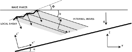
Figure 3: Definition of variables. Three different coordinates systems will be successively used: the gravity-oriented one $(x,z)$, the slope-oriented one $(x^{\prime},z^{\prime})$ and finally the incident beam oriented one ($s,\sigma)$. The PVC sheet compressed periodically along the dotted line provides a shear flow orthogonal to this line, and thus tilted at a constant angle $\Phi$ with the vertical. This flow induces waves propagating at an angle $\theta$ with the horizontal, determined by the dispersion relation (1) while $\alpha$ is the slope angle.

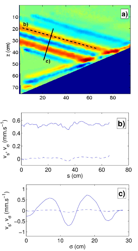
Figure 4: Picture in color. False-color pattern of the along-beam ${v_{s}}(x,z)$ velocity for $\theta=16^{\circ}$ and $\alpha=22^{\circ}$ in a vertical $(x,z)$ section. The shaded triangle corresponds to the region below the glass plate, unperturbed by the internal waves. The maximum velocity in this figure is 0.07 cm.s^-1. Panels (b) and (c) show the along-beam and cross-beam sections respectively, indicated by the dashed and solid lines in panel (a). The longitudinal variation $v_{s}$ is shown in panel (b) and (c) with solid lines, while the dashed lines correspond to the transversal variation $v_{\sigma}$. The longitudinal coordinate $s$ and the transversal one $\sigma$ are defined in Fig. 3.

III Experimental results

III.1 Spectral analysis

An important characteristic of the reflection of internal waves is the generation of different harmonics, theoretically predicted a long time ago [23, 3], but only very recently experimentally observed [17]. However the amplitudes of the different harmonics can be very different and, consequently, hardly distinguishable even though their propagation angles are different. A typical example is presented in Fig. 5a.

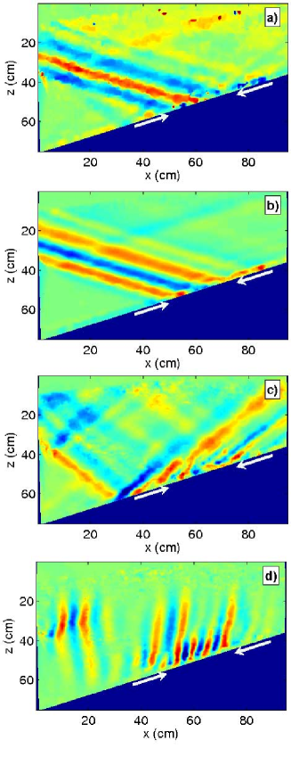
Figure 5: All panels in color. False-color velocity pattern in the vertical $(x,z)$-plane for the critical run 4 (see Table 1). Panel (a) presents the instantaneous horizontal velocity field $u(x,z,t)$ while panel (b) shows the phase-averaged velocity $\langle u\rangle_{1}$. Panels (c) and (d) show respectively the second $\langle w\rangle_{2}$ and third $\langle w\rangle_{3}$ harmonics of the vertical velocity, $\langle w\rangle_{n}$, in the case of run 4 (see Table 1). The two white arrows define the impinging region of the incident beam. In panels (c) and (d), the rays at the left of this region should thus not be taken into account: they have been generated by the screen. The maximum velocity in panels (a) and (b) is 2 mm.s^-1 and, in panels (c) and (d), 0.4 mm.s^-1.

This is the reason why we developed a Fourier temporal analysis of the results, with filtering at the fundamental and higher harmonics frequencies. Given the two components of the velocity field provided by the PIV analysis, we compute the filtered velocity fields. For the horizontal one $u(x,y,t)$, one thus defines the different quantities

$$\langle u\rangle_{n} = \frac{2}{t_{1}-t_{0}}\int_{t_{0}}^{t_{1}}\!\!\!\!u(x,z,t)\cos(n\omega t+\phi)\,\mathrm{d}t.$$ (4)

In the time interval $[t_{0},t_{1}]$, the amplitude of the $n$-th harmonic $\langle u\rangle_{n}$ is of course a function of the spatial variables $x$ and $z$, but also of a constant phase $\phi$, chosen with respect to the flat position of the sinusoidal paddle. This procedure is equivalent to band pass filtering the PIV time series at each point in the domain.

Panels (b), (c) and (d) of Fig. 5 show that this procedure is an excellent tool to distinguish the different harmonics. Indeed, for this almost critical reflection case (run 4, $\alpha=22^{\circ}$, $\theta=22\pm 1^{\circ}$), it is clearly apparent in panel (b), that the reflected beam at frequency $\omega$ is absent except a small slightly supercritical alongslope ray. Nevertheless, panels (c) and (d) show the emitted second and third harmonics propagating with steeper angles. The angles of propagation with respect to the horizontal for the second harmonic beam is $\theta_{2}=48\pm 1^{\circ}$ in agreement with the theoretical value

$$\theta_{n}=\sin^{-1}(n\sin\theta),$$ (5)

for $n=2$. The third harmonic is evanescent; its characteristics will be discussed in Sec. III.3. Both harmonics are generated in the finite domain region, adjacent to the bottom, where the incident beam hits the slope. One should not take into account the few rays located at the left of the arrows (see Figs. 5c and 5d): they were generated by the oscillations of the screen. The emitted second harmonic between the two arrows can still be spatially distinguished from these artifacts. It is important to emphasize that the color scales differ by a factor 5 between the two first panels and the two last ones.

In summary, Figs. 5 exemplified that, even though the second and third harmonics are almost invisible from the instantaneous velocity field, they are very clearly apparent after the filtering procedure. This filtering method is consequently appropriate even when the amplitude is very small. To our knowledge, even if it was previously predicted [23, 21] this is the first case where the third harmonic has been observed, and even more important, this is the first report of experimental quantitative measurements.

It is important to notice that the vertical velocity field is presented in panels (c) and (d), rather than the horizontal one as in the first two panels. Indeed, as the second and third harmonics propagation angles are much steeper, the horizontal velocity field is of lower quality.

An alternative possibility to keep the spatial conformation of the reflection process while distinguishing the different harmonics is to consider the specific kinetic energy density field of each harmonic which can be deduced from Eq. (4) as

$$\langle E\rangle_{n}(x,y,\phi)=\frac{1}{2}\left[\langle u\rangle_{n}^{2}+\langle w\rangle_{n}^{2}\right].$$ (6)

An example is shown in Fig. 6 for the subcritical run 2. One clearly distinguishes the incident beam impinging on the slope, and reflected downslope. It is clear that such energy plots give less contrasted results than the velocity ones as in Figs. 5. They are nevertheless extremely useful for amplitude estimates along cross sections of the beam as discussed below.

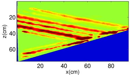
Figure 6: Color online. False-color energy pattern. The specific kinetic energy density of the first harmonic, $\langle E\rangle_{1}$, is shown in the vertical $(x,z)$-plane for the subcritical run 2 (see Table 1). The maximum value is 5.$10^{-3}$ cm².s^-2.

III.2 Mechanism of wavelength selection

The spectral decomposition presented in the previous section allows precise wavelength measurements across the different beams, even in the impact zone. As the reflection surface is expected to play a key role in wavelength selection via boundary effects, we have focused our study in the boundary region along the slope.

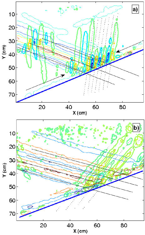
Figure 7: Pictures in color. Superposition of the vertical velocities contourplots of the incident first harmonic (normal) and of the emitted third harmonic (bold). Panel (a) presents the critical case (run 4) while panel (b) shows the subcritical case (run 2). The solid lines show the phase lines of the incident first harmonic $\langle w\rangle_{1}$ while the dashed ones correspond to the phase lines of the emitted third harmonic $\langle w\rangle_{3}$. The two arrows in panel (a) indicate precisely the alongslope cross-section used in Fig. 8.

In Fig. 7(a), the contourplots of the filtered first harmonic (incident) and of the third harmonic (emitted) are superimposed in order to show the alongslope wavelength selection. It is clearly visible that the distance between the emitted phase lines has been strongly reduced compared to the incident ones. We emphasize that the wavelength selection mechanism appears to occur along the slope, where the superposition of the incident and the reflected beams generates nonlinear interactions. Assuming that this inner region plays a key role in the reflection of internal waves [3], the only relevant dynamical behavior of the wave field has to be taken at $z^{\prime}=0$ where the incident and the emitted waves can both be written as $\psi(z^{\prime}=0)=A\exp[i(k_{x^{\prime}}x^{\prime}-\omega t)]$, the amplitude $A$ being different for the incident and the reflected waves. Nonlinear interactions may lead to second or third harmonics terms such as $\psi_{2}(z^{\prime}=0)=A_{2}\exp[2i(k_{x^{\prime}}x^{\prime}-\omega t)]$ or $\psi_{3}(z^{\prime}=0)=A\exp[3i(k_{x^{\prime}}x^{\prime}-\omega t)]$. The alongslope wavelength of the third harmonic is thus reduced by a factor three, as highlighted in Fig. 7(a) by the phase lines intersections with the slope.

To gain further insight, Figs. 8 present quantitative measurements of this effect in the supercritical case 5. The cross sections of the first three harmonics at a fixed distance from the slope are presented. The difference in $x^{\prime}$-location are of pure geometrical origin and decrease, of course, when the cross-section is taken closer to the slope. These pictures are analogous to the theoretical results presented by Tabaei, Akylas and Lamb in Figs. 9(a-d) of Ref. [21].

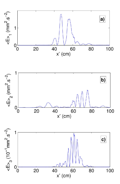
Figure 8: Alongslope sections of the energy of the incident first harmonic (panel a), second harmonic (panel b) and of the emitted third harmonic (panel c) in the supercritical case (run 5). The sections were obtained at 7 cm from the slope, as indicated by the arrows in Fig. 7(a). Note the difference in units for the ordinates.

Let us stress that the above quantitative comparisons are possible despite the large difference between the incident and emitted amplitudes. The automatic elimination of wrong vectors in the measurements by the high quality cross-correlation PIV algorithm (designed by Fincham and Delerce [5]) is the key point here to achieve this goal. The measurements are indeed sufficiently precise to provide meaningful results even when the relative energy ratio between successive harmonics is approximately 0.1. This last ratio is of course directly linked to the parameter $\varepsilon$, used in Refs. [3, 21] for the small amplitude asymptotic expansion to describe theoretically the reflection process. This is consequently not a limiting factor.

The nonlinear wavelength selection can be clearly highlighted using above the three pictures. Indeed, Fig. 9 presents their spatial Fourier transform and clearly emphasizes that the wavelength of the $n$-th harmonic is $n\lambda$, explaining the wavevector tripling visible in Fig. 7(a) as theoretically predicted by Tabaei, Akylas and Lamb [21].

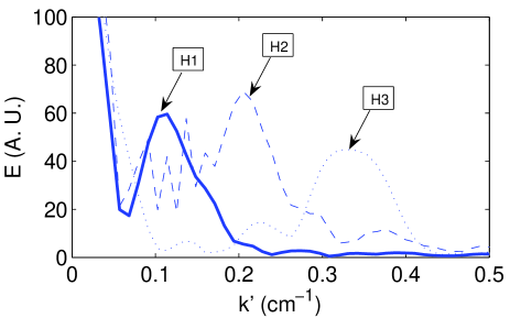
Figure 9: Spatial Fourier transform of the alongslope sections presented in Figs. 8. The solid line corresponds to $<E>_{1}$ (Fig. 8(a)), the dashed one to $<E>_{2}$ (Fig. 8(b)) and the dotted one to $<E>_{3}$ (Fig. 8(c)). This picture emphasizes the frequency tripling.

Experimental results in subcritical cases have unexpectedly revealed an apparent different mechanism for the wavelength selection, when the slope angle $\alpha$ is larger than $\theta$, the angle of energy propagation. A typical example is shown in Fig. 7(b). The second harmonic has disappeared and the wavelength of the third harmonic is equal to the incident wave when it is projected along the slope. This possibility was already mentioned by Thorpe [23] since third order nonlinear interaction along the slope ($z^{\prime}=0$) may lead to third harmonics of the form $\psi_{3}(z^{\prime}=0)=A\exp[i(k_{x^{\prime}}x^{\prime}-3\omega t)]$, where the temporal frequency is tripled while the spatial frequency is kept constant. This is to our knowledge the first experimental evidence of this possible nonlinear interaction. The transition from supercritical (third harmonics alongslope wavevector tripling and second harmonics alongslope wavevector doubling) to subcritical case (third harmonics alongslope wavevector conservation and absence of second harmonics), is visible in Fig. 7(a) where for the critical case, both wavelengths are present at the frequency $3\omega$ (same alongslope wavelength on the left of the impact zone, tripled on the right). However, this transition remains unexplained.

III.3 Evanescent harmonics

The angles of propagation of the different harmonics have been measured on the filtered patterns. All the results are listed in Table 2 for the five runs of Table 1. The values are also plotted in Fig. 10 as a function of the pulsation $\omega$ and of the harmonic number $n$. Panel (a) attests that the first and second harmonic are in perfect agreement with what is theoretically expected: all corresponding symbols are on the straight line $\omega=N\sin\theta$. This is not the case for the third harmonic in the three last runs. When the sine of the propagation angle is plotted versus the number of the harmonic as in panel (b), one also sees that the third harmonic is not aligned with the first two ones for runs 3 to 5.

Run	1	2	3	4	5
$\theta_{1}$ (deg.)	12	16.5	19.5	22.5	25
$\theta_{2}$ (deg.)	26	35	41	48	54
$\theta_{3}$ (deg.)	43	52	?65	85	81.5
$\sin\theta_{1}$	0.21	0.28	0.33	0.38	0.42
$\sin\theta_{2}$	0.44	0.57	0.66	0.74	0.81
$\sin\theta_{3}$	0.68	0.79	0.91	1.00	0.99

Table 2: Experimentally measured angles of propagation for the three different harmonics. The precision of the measures is smaller than half a degree. The characteristics of the five runs are given in Table 1.

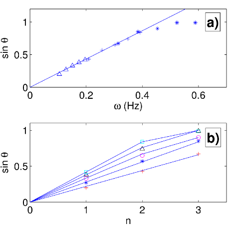
Figure 10: Angular dispersion for the different harmonics. Panel (a) presents the sine of the different angles of propagations versus the wave frequency $\omega$. The different symbols corresponds to the first (triangles), second (plus) and third harmonic (stars). The solid line corresponds to the theoretical law $\omega=N\sin\theta$ for $2\pi N^{-1}=13.6s$. Panel (b) presents the same data as a function of the number of the harmonics for runs 1 to 5, respectively plus, stars, circles, triangles and squares). Error bars are smaller than the symbol size.

As discussed for example by Tabaei et al [21], the maximum incident angle $\theta$ for which the $n$-th harmonic can propagate is $\sin^{-1}(1/n)$. For larger angles, the corresponding harmonic will be evanescent since the frequency would be larger than the Brunt-Väisälä top band frequency. For $\theta>\sin^{-1}(1/3)\simeq 19^{\circ}$, the third harmonic is thus found to be evanescent : this is the case for runs 3, 4 and 5 of Table 2, explaining the three symbols not on the line in Fig. 10(a). In these cases, the third harmonic generated in the impact zone cannot propagate, and is thus trapped along the slope. This is what is shown in Fig. 11. Evanescent modes were also found experimentally [22] in a different context, nonlinear non-resonant interaction between two internal wave rays.

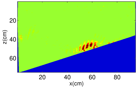
Figure 11: Color online. False-color velocity pattern. The vertical third harmonic $<w>_{3}$ is shown in the $(x,z)$-plane for the run 5. The maximum velocity is 0.4 mm.s^-1.

If the evanescence of the wave is clarified, an angle of propagation, not vertical, can be measured as shown for run 5 in Fig. 11. Another case is also visible in Fig. 5(d). It is possible to theoretically explain this angle as follows.

Considering the linear equation (3) valid for internal waves within the Boussinesq approximation, let us look for streamfunction solutions $\psi$, evanescent in the $z^{\prime}$-direction, i. e. orthogonally to the slope, but propagating in the $x$ and $z$ direction (see Fig. 3 for the definitions of these variables). Introducing the two components of the wavevector $(k_{x},k_{z})$ and $\delta$, the attenuation (or evanescence) length, we thus look for solutions as

$$\psi(x,z,t) \!\!\!\!=\!\!\!\! \psi_{0}\,e^{\displaystyle i(k_{x}x+k_{z}z-\omega t)}\ e^{\displaystyle-{z^{\prime}}/{\delta}}$$ (7)

$$\!\!\!\!=\!\!\!\! \psi_{0}\,e^{\displaystyle(ik_{x}\!\!+\!\!{\sin\alpha}/{\delta})x\!\!+\!\!(ik_{z}\!\!-\!\!{\cos\alpha}/{\delta})z\!\!-\!\!i\omega t},$$ (8)

since $z^{\prime}=z\cos\alpha-x\sin\alpha$. Introducing the above ansatz in Eq. (3) leads to a complex equation. Separating real and imaginary parts and defining $\gamma=\omega/N$, we get

$$\delta^{2} = \frac{\cos^{2}\alpha}{k_{x}^{2}}\ \frac{\gamma^{2}-\sin^{2}\alpha}{\gamma^{2}-1}$$ (9)

$$k_{z} = k_{x}\tan\alpha\left(1-{\gamma^{-2}}\right).$$ (10)

For $\gamma>1$, we can thus define the angle of propagation of the evanescent wave $\theta_{ev}=\mbox{atan}({k_{x}}/{k_{z}})$. Equation (10) leads to

$$\theta_{ev}(\alpha,\gamma)=\mbox{atan}\left(\frac{\mbox{cotan }\alpha}{1-{\gamma^{-2}}}\right).$$ (11)

Figure 12 attests that the experimental results agree very well with formula (11) for run 4 and run 5. Unexpectedly the case $\theta=19^{\circ}$ for which the third harmonic is at the limit of evanescence is however not described by the above model. Note also that an alternative theoretical description is proposed in Ref. [21].

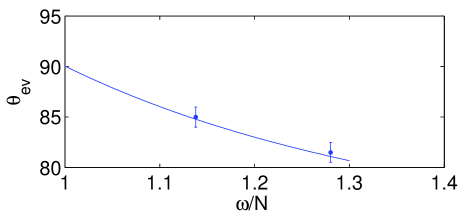
Figure 12: Angle of propagation of the evanescent third harmonic for run 4 and run 5.

III.4 Amplitude measurements

The determination of wave amplitudes is complicated by the beam-like appearance of the displacement field. Indeed, local temporal spectral analysis is not sufficient to provide reliable energy measurements, as phase and group speed are orthogonal. Spatial integration across the beam are needed to accurately evaluate the amounts of energy involved in each harmonics.

First to validate the method of measurement, the mean displacement amplitudes $A=\sqrt{u^{2}+w^{2}}/\omega$ of the incident beam is plotted as a function of the incidence angle. The wavemaker being tilted at a constant angle $\Phi=13^{\circ}$ with the horizontal, it induces a shear motion perpendicular to itself (see Fig. 3). The propagating part of this motion is thus expected to be proportional to $\sin(\theta+\Phi)$. The very good agreement shown in Fig. 13 justifies a posteriori the method.

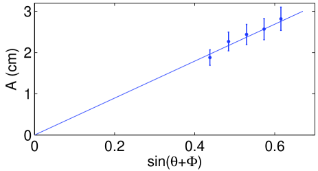
Figure 13: Experimental measure of the displacement amplitude of the emitted wave as a function of the emission angle $\theta$, for the five runs of Table 1.

Determining the importance of the different harmonics emitted after the reflection process is an important issue to understand and hence describe theoretically the reflection process. After exploring several possibilities, it appears that the best method to quantitatively characterize the measurements is the following one. First, it is important to distinguish the two components of velocities vectors, parallel to the slope and orthogonal to it. The second one vanishes clearly close to the slope, satisfying thus the expected boundary conditions. Away from the slope, because of the possibilities of evanescence it is very delicate to get reliable amplitudes. On the contrary, the along slope component of the velocities is easier to deal with. It has no reason to vanish close to the slope and definitely did not. We have thus measured the amplitude of the wave by determining the maximum value of the different harmonics. Results are collected and shown in Fig. 14. The velocity amplitudes for the second and third harmonics are 4 times smaller than for the first harmonic, even for run 4 and run 5 when the third harmonic is evanescent. It is important to emphasize that the difference between the second and third harmonic is small.

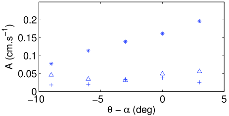
Figure 14: Velocity amplitudes of the first three harmonics as functions of the difference between the emission angle $\theta$ and the slope angle $\alpha$, for the five runs of Table 1. Stars, triangles and crosses correspond to the first, second and third harmonic respectively.

IV Conclusion

In this paper, we have reported quantitative laboratory measurements of the propagation of internal waves. Our experimental set-up produces an incident beam of high quality. Its large scale allows to reach large Reynolds numbers, such that the effects of dissipation on the propagation is negligible. This is not anymore true for the critical reflection mechanism, which involves a strong reduction of the wavelength, hence increased viscous effects. Thus, one obtains a steady regime compatible with the hypothesis of previous theoretical models [3, 21].

The wavevector of the frequency $n$-th harmonics, projected along the slope, is found to be proportional to $n$ in the supercritical case. This is in agreement with the theory [21]. A different selection mechanism is however observed in the sub-critical case, for which the wavenumber is equal to the incident one. This is in contradiction with [21], but in agreement with a more simple analysis previously proposed by Thorpe [23].

Harmonics with frequency higher than $N$ cannot propagate and remain trapped near the slope. We document their existence for the first time and explain their spatial structure.

The long two-dimensional internal waves exciter produces very weak transversal $y$-variations apparently justifying two-dimensional predictions in the $(x,z)$-plane. Considering a rotating tank would require to address the much tougher, fully three dimensional equation and it is not a priori clear what will happen. Work along this line is in progress.

Acknowledgments

We thank G. Delerce and S. Mercier for help during the experiments and post-processing. Comments to the manuscript by Denis Martinand are deeply appreciated. This work has been partially supported by the 2005 PATOM CNRS program and by 2005-ANR project TOPOGI-3D.

References

- [1] D. Cacchione and C. Wunsch. Experimental study of internal waves over a slope. Journal of Fluid Mechanics, 66:223, 1974.
- [2] T. Dauxois, A. Didier, and E. Falcon. Observation of near-critical reflection of internal waves in a stably stratified fluid. Physics of Fluids, 16:6, 2004.
- [3] T. Dauxois and W. R. Young. Near-critical reflection of internal waves. Journal of Fluid Mechanics, 390:271, 1999.
- [4] C. C. Eriksen. Implications of Ocean Bottom Reflection for Internal Wave Spectra and Mixing. Journal of Physical Oceanography, 15:1145, 1985.
- [5] A. Fincham and G. Delerce. Advanced optimization of correlation imaging velocimetry algorithms. Experiments in Fluids, 29:13, 2000.
- [6] L. Gostiaux, N. Garnier, E. Falcon, and T. Dauxois. Generation of internal waves by vibrating cylinders revisited. In preparation, 2005.
- [7] G. N. Ivey and R. I. Nokes. Vertical mixing due to the breaking of critical internal waves on sloping boundaries. Journal of Fluid Mechanics, 204:479, 1989.
- [8] G. N. Ivey, K. B. Winters, and I. P. D. De Silva. Turbulent mixing in a sloping benthic boundary layer energized by internal waves. Journal of Fluid Mechanics, 418:59, 2000.
- [9] A. Javam, J. Imberger, and S. W. Armfield. Numerical study of internal wave reflection from sloping boundaries. Journal of Fluid Mechanics, 396:183, 1999.
- [10] A. Javam, J. Imberger, and S. W. Armfield. Numerical study of internal wave-wave interactions in a stratified fluid. Journal of Fluid Mechanics, 415:65, 2000.
- [11] L. R. M. Maas. Wave focusing and ensuing mean flow due to symmetry breaking in rotating fluids. Journal of Fluid Mechanics, 437:13, 2001.
- [12] L. R. M. Maas, D. Benielli, J. Sommeria, and F.-P. A. Lam. Observation of an internal wave attractor in a confined stably stratified fluid. Nature, 388:557, 1997.
- [13] L. R. M. Maas and F.-P. A. Lam. Geometric focusing of internal waves. Journal of Fluid Mechanics, 300:1, 1995.
- [14] E. E. McPhee-Shaw and E. Kunze. Boundary layer intrusions from a sloping bottom: A mechanism for generating intermediate nepheloid layers. Journal of Geophysical Research, 107:31, 2002.
- [15] D. E. Mowbray and B. S. H. Rarity. A theoretical and experimental investigation of the phase configuration of internal waves of small amplitude in a density-stratified liquid. Journal of Fluid Mechanics, 28:1, 1967.
- [16] A. Fincham O. Praud and J. Sommeria. Decaying grid turbulence in a strongly stratified fluid. Journal of Fluid Mechanics, 522:1, 2005.
- [17] T. Peacock and A. Tabei. Visualization of nonlinear effects in reflecting internal wave beams. Physics of Fluids, 17:061702, 2005.
- [18] O. M. Philipps. The Dynamics of the Upper Ocean. Cambridge University Press, London and New-York, 1977.
- [19] D. N. Slinn and J.J. Riley. Turbulent dynamics of a critically reflecting internal gravitywave. Theoretical and Computational Fluid Dynamics, 11:281, 1998.
- [20] B. R. Sutherland. Propagation and reflection of internal waves. Physics of Fluids, 11:1081, 1999.
- [21] A. Tabaei, T. R. Akylas, and K. Lamb. Nonlinear effects in reflecting and colliding internal wave beams. Journal of Fluid Mechanics, 526:217, 2005.
- [22] S. G. Teoh, G. N. Ivey, and J. Imberger. Laboratory study of the interaction between two internal wave rays. Journal of Fluid Mechanics, 336:91, 1997.
- [23] S. A. Thorpe. On the reflection of a train of finite-amplitude internal waves from a uniform slope. Journal of Fluid Mechanics, 178:279, 1987.
- [24] S. A. Thorpe and A. P. Haines. A note on observations of wave reflection on a 20 degree slope. Journal of Fluid Mechanics, 178:279, 1987.
- [25] O. Zikanov and D. Slinn. Along-slope current generation by obliquely incident internal waves Journal of Fluid Mechanics, 445:235, 2001.