Signature of directed chaos in the conductance of a nanowire

Abstract

We study the conductance of chaotic or disordered wires in a situation where equilibrium transport decomposes into biased diffusion and a counter-moving regular current. A possible realization is a semiconductor nanostructure with transversal magnetic field and suitably patterned surfaces. We find a non-trivial dependence of the conductance on the wire length. It differs qualitatively from Ohm’s law by the existence of a characteristic length scale and a finite saturation value.

According to Ohm’s law, the resistance of a wire is proportional to its length. This is a straightforward consequence of the diffusive motion of electrons in the disordered potential of a normal material. However, unlike the time when Ohm arrived at his fundamental observation, conductors can be tailor-made today with almost complete control over the microscopic structure. Therefore it is important to understand the consequences of non-diffusive electron dynamics on the electronic conductance or other transport properties. This question has been studied in much detail for semiconductor nanostructures in which the motion of electrons is ballistic rather than diffusive Imry ; M+92 ; P+01 ; W+91 . In such systems disorder is negligible and consequently all transport properties are determined by the shape of the sample, as in a billiard model. For example, in the ideal case of a perfectly clean nanowire with parallel walls the resistance should be zero independent of the length, and indeed this remarkable prediction has been confirmed experimentally P+01 . Beside ballistic systems, also the effects of anomalous diffusion on the electronic or thermal conduction properties have attracted a lot of attention FGK94 ; LFL98 ; LW03 .

In the present paper we study the electronic conductance of a wire in the case of a different and very profound modification of the microscopic dynamics. We consider systems where directed chaos leads to biased diffusion in the absence of any potential gradient. Directed chaos means that the time-averaged velocity of chaotic trajectories is non-zero due to broken time-reversal symmetry and due to the specific phase space structure. This effect may occur in various types of systems including, e.g., cold atoms in suitably pulsed optical potentials or chains of electronic billiards in a transversal magnetic field. It has been investigated both, theoretically and experimentally, in a number of recent publications FYZ00 ; S+01 ; M+02 ; AD03 ; SP05 . The interest is due to some intriguing and potentially very useful properties. For example, quantities like velocity average, velocity dispersion or scattering delay times are intrinsically dependent on the transport direction. However, all previous studies focused on the ratchet-like directed transport in effectively infinite periodic systems with directed chaos. In contrast, we address here for the first time the typical electronic setup of a finite sample which is coupled to two electron reservoirs. We show that directed chaos has profound consequences also in this context where the transport velocity is not directly measurable; instead the conductance becomes the most basic and most relevant quantity. Due to biased diffusion, a new length scale $\lambda_{\rm ch}$ appears and rules the asymptotic decay of the conductance with the sample length, see Eq. (10) below. Moreover, chaotic trajectories can propagate through samples of arbitrary length and consequently the conductance approaches a non-zero constant given in Eq. (5). Note that it is not possible to reduce the description of directed chaos to a diffusion equation with bias. In our explicit result for the conductance, Eq. (17), we must account also for the detailed structure of the underlying mixed phase space.

To be specific, we investigate the prototypical model first introduced in SP05 . We consider a two-dimensional electron gas (2DEG) confined to a quasi one-dimensional channel (Fig. 1a). One wall of the channel is straight. Electrons are specularly reflected, but no back scattering occurs in the transport direction. The other wall has a rough surface causing strong and essentially random scattering. The details of this roughness are not crucial (see below). Directed chaos is induced by a perpendicular magnetic field which breaks time-reversal invariance. We stress that a realization of our model does not require more than a novel combination of elements which are all well understood and experimentally accessible in the context of a mesoscopic 2DEG, namely transversal magnetic fields of moderate strength, negligible bulk scattering and surfaces which are either disordered or manufactured with a precisely defined geometry Imry ; M+92 ; P+01 ; W+91 ; FGK94 ; LFL98 .

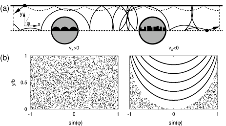
Figure 1: (a) A prototypical example for directed chaos is a 2DEG in a perpendicular magnetic field which is confined by two parallel walls with different surfaces. The upper wall reflects specularly while at the lower wall the reflection angle is essentially random. Possible physical realizations of this randomness are magnified in the insets (see text). Typical trajectories are either regular (dashed line) or random (full line) and transport in opposite directions. In (b) the transversal Poincaré sections for $v_{x}>0$ and $v_{x}<0$ are displayed.

For our purpose it is sufficient to treat the electrons as independent classical particles, i.e., we assume a semiclassical regime with many transversal modes in the channel, $N\sim m^{*}\!v_{\rm F}b/h\gg 1$. We use dimensionless units in which channel width and Fermi velocity are unity, $b=v_{\rm F}=1$. The strength of the magnetic field is parameterized by the cyclotron radius $r_{c}=m^{*}\!v_{\rm F}/eB$. Besides the length of the sample this is the only free parameter in our problem. We will assume that the magnetic field is not too strong, $r_{c}\geq 1$. In this case there are no pinned orbits in the bulk of the channel and the phase space contains only two types of electron trajectories: regular orbits skipping along the clean channel boundary, and chaotic or random orbits which are reflected from both walls (Fig. 1a). The regular orbits are transporting continuously in one direction, say to the left. On the average, the chaotic orbits are transporting in the opposite direction, thus compensating for the regular transport and making the system unbiased as a whole. However, the transport velocity $\dot{x}$ of a chaotic electron is fluctuating, in fact the dynamics is diffusive with a superimposed drift along the channel. The average drift velocity can be obtained by application of a phase space sum rule S+01 . For our model we find for the long-time velocity average of almost all chaotic trajectories

$$v_{\rm ch} = {1\over 2}{\theta-\sin\theta\cos\theta\over\pi(1-\cos\theta)-\sin\theta+\theta\,\cos\theta}$$ (1)

with $\theta(r_{c})=\arccos(1-{1/r_{c}})$ SP05 . This result is independent of the precise modelling of the rough channel surface as long as the phase space structure of Fig. 1b is preserved. In SP05 we considered the two extreme cases shown in the insets of Fig. 1a. In one case the surface is a periodic array of semicircular scatterers with small radius $R\to 0$ , i.e., the dynamics of the system is deterministic and there is no disorder whatsoever. In the second case the direction $\varphi$ of the trajectory was randomized upon every scattering from the rough surface. Specifically it was chosen with probability density $P(\varphi)={1\over 2}{\sin\varphi}$ from the interval $[0,\pi]$ such that the invariant measure on the energy shell $dx\,dy\,d\varphi$ was preserved. A physical realization of this behavior is a disordered surface with a correlation length that is below the Fermi wavelength. While this second system is non deterministic when approximated classically, its transport properties are essentially the same as for the case of deterministic directed chaos. In particular, in both cases an ensemble of chaotic trajectories spreads diffusively around the moving center of mass, $\langle\Delta x^{2}\rangle=D_{\rm ch}t$ SP05 . The precise value of the diffusion constant depends on the detailed modelling of the rough boundary. Analytical results for $D_{\rm ch}$ are available in the case of random scattering SP05 and therefore we shall use this version of the model in the numerical calculations below.

The electronic conductance is obtained within the framework of the Landauer-Büttiker formula Imry , $G(L)=(2e^{2}/h)\,T(L)$. We approximate the transmission semiclassically, $T\sim Nt(L)$, and discuss quantum corrections at the end of this letter. $t(L)$ denotes the total classical probability that an electron is transmitted through a sample of length $L$ if it enters the system at $x=0$ from the left with random initial conditions $P(y,\varphi)={1\over 2}{\cos\varphi}$ ($y\in[0,1]$, $\varphi\in[-{\pi\over 2},+{\pi\over 2}]$). According to our convention (regular orbits are skipping to the left) these initial conditions are within the chaotic component of phase space. Similarly, we define the probability $t^{\prime}(L)$ that an electron is transmitted if it enters at $x=L$ from the right with an analogous distribution (but $\varphi\in[{\pi\over 2},{3\pi\over 2}]$). The total transmission probability must be the same for the two distinct transport directions,

$$t(L)=t^{\prime}(L)\,.$$ (2)

There are various ways to arrive at this fundamental identity. For example, one observes that $t\neq t^{\prime}$ would result in the accumulation of particles in one of the reservoirs even when the system is in thermal equilibrium. Alternatively, a microscopic derivation can be based on the fact that the scattering map of Hamiltonian systems is area preserving. Although Eq. (2) is not specific for directed chaos, this identity has very interesting consequences in the present context. While $t(L)$ is entirely due to chaotic trajectories whose properties are not immediately accessible, $t^{\prime}(L)$ can be decomposed into conditional probabilities for regular and chaotic trajectories,

$$t^{\prime}(L) = \mu_{\rm reg}\,t^{\prime}_{\rm reg}(L)+\mu_{\rm ch}\,t^{\prime}_{\rm ch}(L)\,,$$ (3)

where

$$\mu_{\rm reg}={1\over 2}\int_{\rm reg}dy\,d\varphi\,\cos\varphi={1\over 2}{\theta-\sin\theta\,\cos\theta\over 1-\cos\theta}$$ (4)

is the the relative area of the regular component in the transversal Poincaré section (Fig. 1b), and $\mu_{\rm ch}=1-\mu_{\rm reg}$. Due to the lack of back scattering along the regular trajectories we have $t^{\prime}_{\rm reg}(L)\equiv 1$. Moreover, it is clear that $t^{\prime}_{\rm ch}\to 0$ for $L\to\infty$. This is so because for trajectories which are moving through arbitrarily long samples against the average chaotic flow the time-averaged velocity cannot converge to $v_{\rm ch}$. Hence these trajectories must be of measure zero in phase space. Taken together, the mentioned facts yield a remarkable result which is illustrated in the right inset of Fig. 2: for long systems the probability that a chaotic trajectory transmits from $x=0$ to $x=L$ is given by the relative phase space area occupied by the counter-moving regular trajectories,

$$t(L)\to\mu_{\rm reg}\qquad(L\to\infty)\,.$$ (5)

The goal is now to understand quantitatively how $t^{\prime}_{\rm ch}(L)$ decays from $t^{\prime}_{\rm ch}(0)=1$ to zero as the length of the system increases. The results of numerical simulations for a wide range of values $r_{c}$ are shown in Fig. 2. The data suggest an exponential behavior for long wires. This can be understood after replacing the microscopic dynamics by the Fokker-Planck equation (FPE) for biased diffusion. At $x=0$ and $x=L$ we assume absorbing boundary conditions. The probabilities to reach these exits from a point $0\leq x\leq L$ within the sample are then

$$p^{\prime}_{L}(x) = {e^{-x/\lambda_{\rm ch}}-e^{-L/\lambda_{\rm ch}}\over 1-e^{-L/\lambda_{\rm ch}}}\,,$$ (6)

$$p_{L}(x) = {1-e^{-x/\lambda_{\rm ch}}\over 1-e^{-L/\lambda_{\rm ch}}}\,,$$ (7)

respectively Gardiner . Here

$$\lambda_{\rm ch}=D_{\rm ch}/v_{\rm ch}$$ (8)

denotes the Peclet length of the biased diffusion process.

In order to contribute to the transmission from the right to the left end of a wire of length $L$, a chaotic particle should first be transmitted through a segment of length $l<L$ and then, starting from $x=L-l$, be absorbed at $x=0$. Based on this argument we propose as a recursion relation for the chaotic transmission

$$t^{\prime}_{\rm ch}(L)=t^{\prime}_{\rm ch}(l)\,p^{\prime}_{L}(L-l)\,.$$ (9)

Note that this relation cannot be valid for arbitrary $l$. For example, $l=0$ leads to $t^{\prime}_{\rm ch}(L)=0$ as for a diffusing particle starting at one of the absorbing boundaries the probability to reach the opposite end is identically zero. The reason for this limitation can be understood as follows. Upon replacing the original dynamical system by a 1D FPE we have discarded all information about the momentum of the electron. Strictly speaking it is then impossible even to define a transmission probability since this requires to enter the system with a given direction. Hence, for Eq. (9) to be valid, the length scale for momentum correlations should be negligible compared to the distance from the boundaries, $\lambda_{\rm ch}\ll x$ and $\lambda_{\rm ch}\ll l$. Under this assumption we find to leading order $t^{\prime}_{\rm ch}(L)=t^{\prime}_{\rm ch}(l)\,e^{-(L-l)/\lambda_{\rm ch}}$ with the solution

$$t^{\prime}_{\rm ch}(L)=c\,\exp(-L/\lambda_{\rm ch})\,.$$ (10)

The dashed line in Fig. 2 shows this exponential for $r_{c}=50$ (with suitably chosen prefactor). Indeed the asymptotic decay of the transmission probability is reproduced. However, for short systems the behavior is clearly not exponential. Moreover, even in the asymptotic regime $L\to\infty$ the FPE approach is not accurate enough to predict the prefactor $c$ of the exponential decay . This is no surprise. According to Eq. (10), a different prefactor corresponds to an additive constant in the system length $L$ and this type of error must be expected after discarding the correlation length of the momentum.

Figure 2: The chaotic transmission (+) is compared to Eq. (16) for $r_{c}=200,50,15,10,6,3,2$ (top-bottom). Each data point represents $10^{6}$ trajectories. For $r_{c}=50$ the asymptotic exponential is shown with a dashed line. Left inset: Dependence of the Peclet length on the cyclotron radius. Right inset: For $r_{c}=10$ the total transmission (•) is compared to Eq. (17) and to the asymptotic constant $\mu_{\rm reg}=0.294$.

We conclude that a satisfactory theory for $t^{\prime}_{\rm ch}(L)$ cannot be based on the FPE alone. As an alternative model let us consider a generalization of the persistent random walk Weiss to a biased walk (BPRW): A particle moves with velocity $\pm v_{\rm F}$ and is reflected with direction-dependent probabilities at obstacles with spacing $L_{1}$. For a segment of length $L=nL_{1}$ we denote the transmission and reflection probabilities by $t_{n}=1-r_{n}=t(nL_{1})$ (left to right) and $t^{\prime}_{n}=1-r^{\prime}_{n}=t^{\prime}_{\rm ch}(nL_{1})$ (right to left). A multiple-scattering expansion allows to express these probabilities in terms of a single segment. We find

$$t_{n} = {1-r_{1}^{\prime}/r_{1}\over(t_{1}^{\prime}/t_{1})^{n}-r_{1}^{\prime}/r_{1}},$$ (11)

$$t^{\prime}_{n} = {1-r_{1}/r_{1}^{\prime}\over(t_{1}/t_{1}^{\prime})^{n}-r_{1}/r_{1}^{\prime}}\,.$$ (12)

In our case the chaotic transport is biased to the right. Therefore we assume $t_{1}>t_{1}^{\prime}$ and find in the limit $n\to\infty$

$$t_{\infty}=1-r_{1}/r_{1}^{\prime}$$ (13)

and

$$t_{n}^{\prime}=t_{\infty}\,({t_{1}/t_{1}^{\prime}})^{-n}\qquad(n\to\infty)\,.$$ (14)

However, there is no direct connection between the parameters of the BPRW and the dynamics of our original model. In order to close this gap we must make use of the information about the underlying phase space structure, Eq. (5), and the result obtained within the FPE approach, Eq. (10). The former implies $t_{\infty}=\mu_{\rm reg}$ or equivalently $r_{1}/r_{1}^{\prime}=\mu_{\rm ch}$. Further the comparison of Eqs. (10) and (14) yields

$$c\,\exp(-nL_{1}/\lambda_{\rm ch})=\mu_{\rm reg}\,(t_{1}/t_{1}^{\prime})^{-n}\,.$$ (15)

Now it is easy to read off the correct prefactor of the asymptotic exponential decay, $c=\mu_{\rm reg}$, which was used for the dashed line in Fig. 2. On the other hand we infer $\exp(L_{1}/\lambda_{\rm ch})=t_{1}/t_{1}^{\prime}$ which is substituted into Eqs. (11) and (12). The final result for the chaotic transmission probability from right to left is then

$$t^{\prime}_{\rm ch}(L)={\mu_{\rm reg}\over\exp(L/\lambda_{\rm ch})-\mu_{\rm ch}}$$ (16)

while the total transmission is given by

$$t(L)={\mu_{\rm reg}\over 1-\mu_{\rm ch}\,\exp(-L/\lambda_{\rm ch})}\,.$$ (17)

This non-trivial prediction, which does not contain any free parameters, is confirmed numerically in Fig. 2. The fact that an appropriate synthesis between FPE and BPRW should be used to reproduce the data was not at all obvious. Note that in an analogous approach to the unbiased case the PRW yields Ohm’s law in the form $t(L)=(D/v_{\rm F})L^{-1}$ $(L\to\infty)$ while the FPE implies only $t\sim L^{-1}$. In contrast, for the biased case both approaches contribute complementary information and are in fact mutually incompatible approximations .

Small but systematic deviations are visible in Fig. 2 for both, very small and very large cyclotron radius. At least partially these deviations can be attributed to direct trajectories which escape from the system before being scattered. Such trajectories are always sensitive to the details of a given model and therefore not of primary interest here. We restrict the discussion to some simple examples. Trajectories which enter at $x=0$ with a steep angle $-\pi/2\lesssim\varphi$ will reach $x=0$ again after completing a simple arc. From the geometric condition $\cos\varphi<y/2r_{c}$ we see that the corresponding phase space volume vanishes as $r_{c}^{-1}$. Therefore these trajectories lead to deviations for small cyclotron radius. For short systems or for large cyclotron radius and shallow incidence $\varphi\approx 0$ there can also be directly transmitted trajectories. A rough estimate requires $L\lesssim\sqrt{8r_{c}}$ for their existence which is compatible with Fig. 2 ($L=40$ for $r_{c}=200$).

According to Eq. (17) the conductance of a wire with directed chaos saturates to a finite value as $L\to\infty$. This claim is in sharp contrast to quantum localization which leads to vanishing conductance in any coherent quasi 1D quantum system with uncorrelated disorder. These two contradicting statements can be reconciled as follows. In the presence of directed chaos the localization length $\xi$ diverges exponentially with the number of transversal modes ($\ln\xi\sim N\sim h^{-1}$) H+02 . Thus, even for moderate $N$, the localization length will easily exceed the sample length $L$ or the coherence length of the given material. In this regime we can safely ignore localization. Other quantum effects like weak localization or tunneling are not expected to change our results qualitatively although they may lead to small corrections $\sim N^{-1}$ in the relevant parameters $\lambda$ and $\mu_{\rm reg}$. A numerical analysis of such effects will be attempted elsewhere.

References

- (1) Y. Imry. Introduction to mesoscopic physics. Oxford University Press, Oxford, 1997.
- (2) C. M. Marcus et al. Phys. Rev. Lett., 69:506, 1992; A. G. Huibers et al. Phys. Rev. Lett., 81:1917, 1998.
- (3) R. de Picciotto et al. Nature, 411:51, 2001.
- (4) D. Weiss et al. Phys. Rev. Lett., 66:2790, 1991; Phys. Rev. Lett., 70:4118, 1993.
- (5) R. Fleischmann, T. Geisel, and R. Ketzmerick. Europhys. Lett., 25:219, 1994.
- (6) M. Leadbeater, V. I. Falko, and C. J. Lambert. Phys. Rev. Lett., 81:1274, 1998.
- (7) B. W. Li and J. Wang. Phys. Rev. Lett., 91:044301, 2003; S. Denisov, J. Klafter, and M. Urbakh. Phys. Rev. Lett., 91:194301, 2003.
- (8) S. Flach, O. Yevtushenko, and Y. Zolotaryuk. Phys. Rev. Lett., 84:2358, 2000.
- (9) H. Schanz et al. Phys. Rev. Lett., 87:070601, 2001; H. Schanz, T. Dittrich, and R. Ketzmerick. Phys. Rev. E, 71:026228, 2005.
- (10) T. S. Monteiro et al. Phys. Rev. Lett., 89:194102, 2002; P. H. Jones et al. Preprint physics/0504096, 2005.
- (11) W. Acevedo and T. Dittrich. Prog. Theor. Phys. Suppl., 150:313, 2003.
- (12) H. Schanz and M. Prusty. J. Phys. A, 38:10085, 2005.
- (13) C. W. Gardiner. Handbook of Stochastic Methods. Springer series in synergetics. Springer, Berlin, 1996.
- (14) G. H. Weiss. Aspects and Applications of the Random Walk. North-Holland, Amsterdam, 1994; G. H. Weiss. Physica A, 311:381, 2002.
- (15) L. Hufnagel et al. Phys. Rev. Lett., 89:154101, 2002.