The B-quadrilateral lattice, its transformations
and the algebro-geometric construction

Abstract.

The B-quadrilateral lattice (BQL) provides geometric interpretation of Miwa’s discrete BKP equation within the quadrialteral lattice (QL) theory. After discussing the projective-geometric properties of the lattice we give the algebro-geometric construction of the BQL ephasizing the role of Prym varieties and the corresponding theta functions. We also present the reduction of the vectorial fundamental transformation of the QL to the BQL case.

1. Introduction

During last years the many results describing the well known connection between integrable partial differential equations and the differential geometry of submanifolds have been transfered to the discrete (difference) level, see for example [4, 19, 43]. The interest in such a research is stimulated from various fields, like computer visualization, combinatorics, lattice models in statistical mechanics and quantum field theory, and recent developments in quantum gravity.

A succesful general approach towards description of the relation between integrability and geometry is provided by the theory of multidimensional quadrilateral lattices (QLs) [17]. These are just maps $x:{\mathbb{Z}}^{N}\to{\mathbb{P}}^{M}$ ($3\leq N\leq M$) with planar elementary quadrilaterals. The integrable partial difference equation counterpart of the QLs are the discrete Darboux equations (see Section 2.4 for details), being found first [6] as the most general difference system integrable by the $\bar{\partial}$ method. It should be metioned that the (differential) Darboux equations [11] play an important role [7] in the multicomponent Kadomtsev–Petviashvilii (KP) hierarchy, which is commonly considered [12, 27] as the fudamental system of equations in integrability theory.

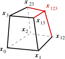
Figure 1. The geometric integrability scheme

It turns out that integrability of the discrete Darboux system is encoded in a very simple geometric statement (see Fig. 1).

Lemma 1 (The geometric integrability scheme).

Consider points $x_{0}$, $x_{1}$, $x_{2}$ and $x_{3}$ in general position in ${\mathbb{P}}^{M}$, $M\geq 3$. On the plane $\langle x_{0},x_{i},x_{j}\rangle$, $1\leq i<j\leq 3$ choose a point $x_{ij}$ not on the lines $\langle x_{0},x_{i}\rangle$, $\langle x_{0},x_{j}\rangle$ and $\langle x_{i},x_{j}\rangle$. Then there exists the unique point $x_{123}$ which belongs simultaneously to the three planes $\langle x_{3},x_{13},x_{23}\rangle$, $\langle x_{2},x_{12},x_{23}\rangle$ and $\langle x_{1},x_{12},x_{13}\rangle$.

Integrable reductions of the quadrilateral lattice (and thus of the discrete Darboux equations) arise from additional constraints which are compatible with geometric integrability scheme (see, for example [15, 18]). One of the most important reductions of the KP hierarchy of nonlinear equations is the so called BKP hierarchy [13] (here ”B” appears in the context of the classification theory of simple Lie algebras). In [34] it was shown that the $\tau$-function of the BKP hiererchy satisfies certain bilinear discrete equation (the transformation between the infinite sequence of times of the hierarchy and the corresponding discrete variables is called the Miwa transformation)

(1.1) $$\tau\,\tau_{(123)}=\tau_{(12)}\tau_{(3)}-\tau_{(13)}\tau_{(2)}+\tau_{(23)}\tau_{(1)},$$

which is known as the discrete BKP or the Miwa equation. Here and in all the paper, given a fuction $F$ on ${\mathbb{Z}}^{N}$, we denote its shift in the $i$th direction in a standard manner: $F_{(i)}(n_{1},\dots,n_{i},\dots,n_{N})=F(n_{1},\dots,n_{i}+1,\dots,n_{N})$.

The linear problem and the Darboux-type (Moutard) transformations for the discrete BKP equation (1.1) were constructed in [38]. In literature there are known several geometric interpretations of the discrete BKP equation in terms of the reciprocal figures and inversive geometry [29, 43], or in terms of the trapezoidal nets [4]. It should be also mentioned that the discrete BKP equation has been recently investigated, under the name of the cube recurrence, in combinatorics [40, 25, 8].

In this paper we propose (see Section 2) another geometric interpretation of the discrete BKP equation, which we consider from the point of view of the quadrilateral lattice theory. This new reduction of the quadrilateral lattice, which we call the B-quadrilateral lattice (BQL), is projectively invariant and is based on additional local linear constraint. Section 2 is of rather elementary geometric nature, but the results obtained there have far reaching consequences. In fact, the paper gives new arguments supporting the conjecture that basic integrability features are consequences of incidence geometry statements (see also introductory remarks in [19]).

More involved techniques are used in Section 3, where we elaborate the algebro-gemetric method to produce large classes of the B-quadrilateral lattices and the corresponding solutions of the discrete BKP system of equations. In doing that we start from recent results of [22], where restrictions on the algebro-geometric data of the discrete Darboux system [1] compatible with the discussed reduction were given. Then we proceed to formulas for the wave and $\tau$-functions of the BQL in terms of the Prym theta functions related with the algebraic curves used in the construction. We transfer this way the algebro-geometric method of construction of solutions of the BKP hierarchy [14] and of its two-component generalization [47] to the discrete level.

We also present, in Section 4, the corresponding reduction of the vectorial fundamental transformation of the quadrilateral lattice [21] and establish its link with the Pfaffian form of the vectorial Moutard transformation found in [38]. In Appendix we give alternative proof of a crucial auxilliary result of the paper, and we summarize basic properties of Pfaffians.

2. The B-quadrilateral lattice

We start with discussing the gometric constraint, which imposed on the quadrilateral lattice allows to define its new integrable reduction. Then we proceed to the algebraic description of such reduced lattice showing its connection with the discrete BKP equation. Finally, we discuss relation between the $\tau$-function of the B-quadrilateral lattice, and the $\tau$-function of the quadrilateral lattice.

2.1. Geometric definition of the BQL

Proposition 2.

Under hypothesess of Lemma 1, assume that the points $x_{0}$, $x_{12}$, $x_{13}$, $x_{23}$ are coplanar, then the points $x_{1}$, $x_{2}$, $x_{3}$, and $x_{123}$ are coplanar as well (see Figure 2).

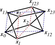
Figure 2. Elementary hexahedron of the B-quadrilateral lattice

It can be shown by the standard linear algebra (for a synthetic-geometry proof see a remark below). We perform however the calculations, because the way we are going to do it will be important in next Sections in showing connection of the BQL with the discrete BKP equation.

Lemma 3.

Under hypotheses of Proposition 2, for fixed initially homogeneous coordinates $\boldsymbol{x}_{0}$ and $\boldsymbol{x}_{1}$ (gauges) of $x_{0}$ and $x_{1}$, there exist a gauge such that the following linear relations hold

(2.1) $$\boldsymbol{x}_{ij}-\boldsymbol{x}_{0}=f^{ij}(\boldsymbol{x}_{i}-\boldsymbol{x}_{j}),\quad 1\leq i<j\leq 3,$$

where the coefficients $f^{ij}$ depend on the actual positions of the points $x_{ij}$.

Proof.

The coplanarity of the four points $x_{0}$, $x_{1}$, $x_{2}$ and $x_{12}$ can be algebraically expressed as the linear relation

$$\alpha\boldsymbol{x}_{0}+\beta\boldsymbol{x}_{1}+\gamma\boldsymbol{x}_{2}+\delta\boldsymbol{x}_{12}=0,$$

where, by the genericity assumption (no three of the points are collinear), all the coefficients do not vanish. By plaing with rescalling the homogeneous coordinates of $x_{2}$ and $x_{12}$ we can transfer above equation to the form (2.1)

(2.2) $$\boldsymbol{x}_{12}-\boldsymbol{x}_{0}=f^{12}(\boldsymbol{x}_{1}-\boldsymbol{x}_{2}).$$

Similarly, we can rescale the homogeneous coordinates of $x_{3}$ and $x_{13}$ to express planarity of the corresponding elementary quadrilateral as

(2.3) $$\boldsymbol{x}_{13}-\boldsymbol{x}_{0}=f^{13}(\boldsymbol{x}_{1}-\boldsymbol{x}_{3}).$$

However, with fixed gauges $\boldsymbol{x}_{0}$, $\boldsymbol{x}_{2}$ and $\boldsymbol{x}_{3}$ the coplanarity of $x_{0}$, $x_{2}$, $x_{3}$ and $x_{23}$ can be expressed, by plaing with the gauge of $\boldsymbol{x}_{23}$, at most as

(2.4) $$\boldsymbol{x}_{23}-\boldsymbol{x}_{0}=a\boldsymbol{x}_{2}-b\boldsymbol{x}_{3}.$$

Then

(2.5) $$\boldsymbol{x}_{0}\wedge\boldsymbol{x}_{12}\wedge\boldsymbol{x}_{13}\wedge\boldsymbol{x}_{23}=f^{12}f^{13}(a-b)\boldsymbol{x}_{0}\wedge\boldsymbol{x}_{1}\wedge\boldsymbol{x}_{2}\wedge\boldsymbol{x}_{3},$$

and at this moment we use coplanarity of $x_{0}$, $x_{2}$, $x_{13}$, $x_{23}$, which is equivalent to $a=b$. ∎

Remark.

Notice that the whole reasoning can be applied even if the gauges of $\boldsymbol{x}_{0}$ and of $\boldsymbol{x}_{1}$ are not fixed initially (we could then achieve $f^{12}=1$). However we will need this additional restriction in next Sections.

Proof of Proposition 2.

By the linear algebra, the homogeneous coordinates of the point $x_{123}\in\langle x_{3},x_{13},x_{23}\rangle\cap\langle x_{2},x_{12},x_{23}\rangle\cap\langle x_{1},x_{12},x_{13}\rangle$, in the gauge of Lemma 3 read

$$\frac{1}{\rho}\boldsymbol{x}_{123}=\left(f^{13}-f^{12}+\frac{f^{12}f^{13}}{f^{23}}\right)\boldsymbol{x}_{1}-\left(f^{23}+f^{12}-\frac{f^{12}f^{23}}{f^{13}}\right)\boldsymbol{x}_{2}+\left(f^{13}-f^{23}+\frac{f^{13}f^{23}}{f^{12}}\right)\boldsymbol{x}_{3},$$

(we still keep the undetermined yet factor $\rho$) which gives coplanarity of $x_{123}$, $x_{1}$, $x_{2}$ and $x_{3}$. ∎

Corollary 4.

By fixing the gauge function $\rho$ to

$$\rho=2f^{13}-2f^{12}-f^{23}+\frac{f^{13}f^{23}}{f^{12}}+\frac{f^{12}f^{13}}{f^{23}}+\frac{f^{12}f^{23}}{f^{13}},$$

we find that the linear relations on the new facets (containing $x_{123}$) of the cube are of the form (2.1) again, for example

$$\boldsymbol{x}_{123}-\boldsymbol{x}_{1}=f^{23}_{1}(\boldsymbol{x}_{12}-\boldsymbol{x}_{13}),$$

where

$$f^{23}_{1}=\frac{f^{23}}{f^{12}f^{13}-f^{12}f^{23}+f^{13}f^{23}}.$$

Remark.

For a geometrically oriented Reader we would like to comment on another interpretation of Proposition 2. It is related to the notion (see, for example [10]) of the quadrangular set of points which are the intersection points of the lines of a complete quadrilateral (add the diagonals). Such a configuration is usually denoted by $\mathsf{Q}(ABC,DEF)$, where the first three points $A,B,C$ lie on sides through one vertex while the remaining three $D,E,F$ lie on the respectively opposite sides, which form a triangle. It is known that $\mathsf{Q}(ABC,DEF)$ implies $\mathsf{Q}(DEF,ABC)$.

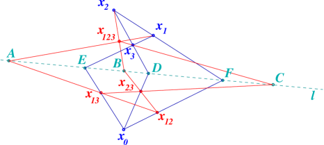
Figure 3. Two quadrangles

In notation of Proposition 2, denote by $\ell$ the intersection line of the plane $\langle x_{1},x_{2},x_{3}\rangle$ with the plane $\langle x_{12},x_{23},x_{13}\rangle$ (containing also the point $x_{0}$). Denote by $A$, $B$, $C$, $D$, $E$, $F$ intersections of sides of the complete quadrilateral with vertices $x_{0},x_{12},x_{23},x_{13}$ with $\ell$ (see Figure 3), i.e. $\mathsf{Q}(DEF,ABC)$. The statement of the Lemma is equivalent to the fact that the lines $\langle A,x_{1}\rangle$, $\langle B,x_{2}\rangle$, $\langle C,x_{3}\rangle$ intersect in one point (which is $x_{123}$); see Excercise 1 of Section 2.4 of [10].

Remark.

As it was pointed to me by Yuri Suris, Proposition 2 is equivalent to the Möbius theorem [35] on mutually inscribed tetrahedra. Indeed, vertices $x_{0}$, $x_{1}$, $x_{2}$, $x_{3}$ of the tetrahedron $\{x_{0},x_{1},x_{2},x_{3}\}$ are contained in the facial planes of the tetrahedron $\{x_{12},x_{13},x_{23},x_{123}\}$, and vice versa. In fact, Figure 3 appears in Möbius’ original proof of the theorem.

Remark.

Proposition 2 can be also considered as a special version of the Miquel theorem [39] (used in [9] to show integrability of the circular lattice) in the same way like Pappus’ hexagon theorem is a special case of the Pascal theorem.

We conclude this Section by defining new reduction of the quadrilateral lattice.

Definition 1.

A quadrilateral lattice $x:{\mathbb{Z}}^{N}\to{\mathbb{P}}^{M}$ is called the B-quadrilateral lattice if for any triple of different indices $i,j,k$ the points $x$, $x_{(ij)}$, $x_{(jk)}$ and $x_{(ik)}$ are coplanar.

Corollary 5.

In the B-quadrilateral lattice, for any triple of different indices $i,j,k$ the points $x_{(i)}$, $x_{(j)}$, $x_{(k)}$ and $x_{(ijk)}$ are coplanar.

2.2. Multidimensional consistency of the BQL constraint

As it was shown in [17] the planarity condition, which allows to construct the point $x_{123}$ as in Lemma 1, does not lead to any further restrictions if we increase dimension of the lattice. This is the consequence of the of the following geometric observation.

Lemma 6.

Consider points $x_{0}$, $x_{1}$, $x_{2}$, $x_{3}$ and $x_{4}$ in general position in ${\mathbb{P}}^{M}$, $M\geq 4$. Choose generic points $x_{ij}\in\langle x_{0},x_{i},x_{j}\rangle$, $1\leq i<j\leq 4$, on the corresponding planes, and using the planarity condition construct the points $x_{ijk}\in\langle x_{0},x_{i},x_{j},x_{k}\rangle$, $1\leq i<j<k\leq 4$ – the remaining vertices of the four (combinatorial) cubes. Then the intersection point $x_{1234}$ of the three planes

$$\langle x_{12},x_{123},x_{124}\rangle,\;\langle x_{13},x_{123},x_{134}\rangle,\;\langle x_{14},x_{124},x_{134}\rangle\quad\text{in}\quad\langle x_{1},x_{12},x_{13},x_{14}\rangle,$$

coincides with the intersection point of the three planes

$$\langle x_{12},x_{123},x_{124}\rangle,\;\langle x_{23},x_{123},x_{234}\rangle,\;\langle x_{24},x_{124},x_{234}\rangle,\quad\text{in}\quad\langle x_{2},x_{12},x_{23},x_{24}\rangle,$$

which is the same as the intersection point of the three planes

$$\langle x_{13},x_{123},x_{134}\rangle,\;\langle x_{23},x_{123},x_{234}\rangle,\;\langle x_{34},x_{134},x_{234}\rangle,\quad\text{in}\quad\langle x_{3},x_{13},x_{23},x_{34}\rangle,$$

and the intersection point of the three planes

$$\langle x_{14},x_{124},x_{134}\rangle,\;\langle x_{24},x_{124},x_{234}\rangle,\;\langle x_{34},x_{134},x_{234}\rangle,\quad\text{in}\quad\langle x_{4},x_{14},x_{24},x_{34}\rangle.$$

Remark.

In fact, the point $x_{1234}$ is the unique intersection point of the four three dimensional subspaces $\langle x_{1},x_{12},x_{13},x_{14}\rangle$, $\langle x_{2},x_{12},x_{23},x_{24}\rangle$, $\langle x_{3},x_{13},x_{23},x_{34}\rangle$, and $\langle x_{4},x_{14},x_{24},x_{34}\rangle$ of the four dimensional subspace $\langle x_{0},x_{1},x_{2},x_{3},x_{4}\rangle$. This observation generalizes naturally to the case of more dimensional hypercube with the planar facets.

The goal of this Section is to show an analogous result for B-quadrilateral lattice. Notice, that in previously known reductions of the quadrilateral lattice, such as the symmetric [18] or the quadratic [15] reduction, the additional constraint was imposed on initial quadrilaterals. Then the multidimensional consistency of the reduction was the result of the three dimensional consistency of the constraint and the multidimensional consistency of the quadrilateral lattice.

In the BQL case, the constraint is imposed on the level of elementary cubes. Therefore its four dimensional consistency is crucial for integrability of the B-quadrilateral lattice, and once proven, implies consistency of the reduction in more dimensions.

Proposition 7.

Under hypotheses of Lemma 6, assume that the BQL condition holds for the initial data, i.e., the point $x_{0}$ belongs to the four planes $\langle x_{ij},x_{ik},x_{jk}\rangle$, $1\leq i<j<k\leq 4$. Then all the three dimensional (combinatorial) cubes obtained in the construction satisfy the BQL constaint, i.e.,

$$x_{1}\in\langle x_{123},x_{124},x_{134}\rangle,\quad x_{2}\in\langle x_{123},x_{124},x_{234}\rangle,\quad x_{3}\in\langle x_{123},x_{134},x_{234}\rangle,\quad x_{4}\in\langle x_{124},x_{134},x_{234}\rangle.$$

Proof.

Consider the gauge of Lemma 3. If we add into the construction points $x_{4}$ and $x_{14}$, then by fixing suitably their gauges $\boldsymbol{x}_{4}$ and $\boldsymbol{x}_{14}$, we can rewrite the coplanarity condition of $x_{0}$, $x_{1}$, $x_{4}$ and $x_{14}$ in the form (2.1). The same argument like in the proof of Lemma 3 implies that the algebraic coplanarity conditions of $x_{0}$, $x_{i}$, $x_{4}$ and $x_{i4}$, $i=2,3$ take the form of equation (2.1).

By fixing gauges of points $x_{ijk}$ like in Corollary 4, we obtain the relations

(2.6) $$\boldsymbol{x}_{ijk}-\boldsymbol{x}_{i}=f^{jk}_{i}(\boldsymbol{x}_{ij}-\boldsymbol{x}_{ik}),\qquad i,j,k\quad\text{disctinct},$$

where

(2.7) $$f^{jk}_{i}=\frac{f^{jk}}{f^{ij}f^{ik}-f^{ij}f^{jk}+f^{ik}f^{jk}},$$

with $f^{ji}=-f^{ij}$.

In equations (2.6) let us fix $i=1$ and consider the three pairs $(j,k)$: $(2,3)$, $(2,4)$ and $(3,4)$. Then after simple calculation we obtain the following linear relation

(2.8) $$f^{24}_{1}f^{34}_{1}(\boldsymbol{x}_{123}-\boldsymbol{x}_{1})-f^{23}_{1}f^{34}_{1}(\boldsymbol{x}_{124}-\boldsymbol{x}_{1})+f^{23}_{1}f^{24}_{1}(\boldsymbol{x}_{134}-\boldsymbol{x}_{1})=0,$$

which shows that $x_{1}\in\langle x_{123},x_{124},x_{134}\rangle$. Other cases are similar. ∎

Corollary 8.

Under assumptions of Proposition 7, the point $x_{1234}$ belongs to the four planes: $\langle x_{12},x_{13},x_{14}\rangle$, $\langle x_{12},x_{23},x_{24}\rangle$, $\langle x_{13},x_{23},x_{34}\rangle$ and $\langle x_{14},x_{24},x_{34}\rangle$.

Remark.

The same procedure can be applied when we increase dimension of the hypercube keeping the BQL constraint.

2.3. BQL and the discrete BKP equation

Proposition 9.

A quadrilateral lattice $x:{\mathbb{Z}}^{N}\to{\mathbb{P}}^{M}$ is a B-quadrilateral lattice if and only if it allows for a homogoneous representation $\boldsymbol{x}:{\mathbb{Z}}^{N}\to{\mathbb{R}}^{M+1}_{*}$ satisfying the system of discrete Moutard equations (the discrete BKP linear problem)

(2.9) $$\boldsymbol{x}_{(ij)}-\boldsymbol{x}=f^{ij}(\boldsymbol{x}_{(i)}-\boldsymbol{x}_{(j)}),\quad 1\leq i<j\leq N,$$

for suitable functions $f^{ij}:{\mathbb{Z}}^{N}\to{\mathbb{R}}$.

Proof.

As we have shown above (we present an alternative difference-equation theory proof in the Appendix), the B-quadrilateral lattices indeed allow for such a gauge; here the Remark after Lemma 3 turns out to be important. Conversely, three equations (2.9) for the pairs $(i,j)$, $(i,k)$, $(j,k)$ imply the linear relation

(2.10) $$f^{jk}f^{ik}(\boldsymbol{x}_{(ij)}-\boldsymbol{x})+f^{ij}f^{ik}(\boldsymbol{x}_{(jk)}-\boldsymbol{x})-f^{ij}f^{jk}(\boldsymbol{x}_{(ik)}-\boldsymbol{x})=0,\qquad 1\leq i<j<k\leq N,$$

expressing coplanarity of the four points $x$, $x_{(ij)}$, $x_{(jk)}$ and $x_{(ik)}$. ∎

The system (2.9) is well known in the literature [38]. Its compatibility leads to the following set of nonlinear equations

(2.11) $$1+f^{jk}_{(i)}(f^{ij}-f^{ik})=f^{ik}_{(j)}f^{ij}=f^{ij}_{(k)}f^{ik},\qquad i,j,k\quad\text{distinct},$$

with $f^{ji}=-f^{ij}$.

Remark.

The system (2.10) can be actually solved, see for example [4], (we have used this fact in a hidden form already). Simply replace the lower index $i$ in the ”star-triangle” relation (2.7) by the shift $(i)$.

On the other side, the second equality in the compatibility condition implies existence of the potential $\tau:{\mathbb{Z}}^{N}\to{\mathbb{R}}$, in terms of which the functions $f^{ij}$ can be written as

(2.12) $$f^{ij}=\frac{\tau_{(i)}\tau_{(j)}}{\tau\,\tau_{(ij)}},\qquad i\neq j.$$

The first equality can be then rewritten in the form of the system of the discrete BKP equations [34]

(2.13) $$\tau\,\tau_{(ijk)}=\tau_{(ij)}\tau_{(k)}-\tau_{(ik)}\tau_{(j)}+\tau_{(jk)}\tau_{(i)},\quad 1\leq i<j<k\leq N.$$

Remark.

Two dimensional quadrilateral lattices whose homogeneous coordinates satisfy (up to a gauge) equation (2.9) are characterized geometrically [22] by condition that any point $x$ and its four second-order neighbours $x_{(\pm 1\pm 2)}$ are contained in a subspace of dimension three. Obviously, any two dimensional slide of the B-quadrilateral lattice fulfills this property, which can therefore serve as definition of a two dimensional BQL. However the example of the standard injection ${\mathbb{Z}}^{N}\to{\mathbb{R}}^{N}\subset{\mathbb{P}}^{N}$ shows that without additional requirements this property does not characterize completly multidimensional BQL.

2.4. The $\tau$-functions

In this Section we present relation between the $\tau$-function of the quadrilateral lattice [18], which we donote here by $\tilde{\tau}$, and the above $\tau$-function of the B-quadrilateral lattice. From the relation between the KP and BKP hierarchies [12] we expect that within the class of the B-quadrilateral lattices $\tilde{\tau}$ should be equal to the square of $\tau$.

Let us recall briefly the algebraic construction of the $\tau$-function of the quadrilateral lattice (the geometric meaning is presented in [18]). The non-homogeneous coordinates $\mathrm{\boldsymbol{x}}:{\mathbb{Z}}^{N}\to{\mathbb{R}}^{M}$ (we restrict our attention to the affine geometric aspects of the theory) of the quadrilateral lattice satisfy the system of Laplace equations

(2.14) $$\boldsymbol{x}_{(ij)}-\boldsymbol{x}=a^{ij}(\boldsymbol{x}_{(i)}-\boldsymbol{x})+a^{ji}(\boldsymbol{x}_{(j)}-\boldsymbol{x}),\quad i\neq j.$$

The functions $a^{ij}:{\mathbb{Z}}^{N}\to{\mathbb{R}}$ are not arbitrary (the system (2.14) must be compatible), in particular they can be parametrized in terms of the potentials $h^{i}$ (the Lamé coefficients) as follows

(2.15) $$a^{ij}=\frac{h_{i(j)}}{h_{i}},\quad i\neq j.$$

Define the so called rotation coefficients $\beta_{ij}$ from equations

(2.16) $$\Delta_{i}h_{j}=h_{i(j)}\beta_{ij},\quad i\neq j,$$

and the normalized tangent vectors $\boldsymbol{X}_{i}$ from

(2.17) $$\Delta_{i}\boldsymbol{x}=h_{i}\boldsymbol{X}_{i}.$$

Then the Laplace system (2.14) takes the first order form

(2.18) $$\Delta_{j}\boldsymbol{X}_{i}=\beta_{ij}\boldsymbol{X}_{j},\quad i\neq j,$$

and its compatibility reads

(2.19) $$\Delta_{j}\beta_{ik}=\beta_{ij(k)}\beta_{jk},\quad i,j,k\quad\text{distinct}.$$

The discrete Darboux equations (2.19) imply existence of the potential $\tilde{\tau}$ (the $\tau$-function of the quadrilateral lattice)

(2.20) $$\frac{\tilde{\tau}\tilde{\tau}_{(ij)}}{\tilde{\tau}_{(i)}\tilde{\tau}_{(j)}}=1-\beta_{ij}\beta_{ji},\quad i\neq j.$$

In looking for the Lamé coefficients $h_{i}$ in the reduction from QL to BQL we can compare both linear systems (2.9) and (2.14), and the expresions (2.15) and (2.12) to obtain

(2.21) $$h_{i}=(-1)^{\sum_{k<i}m_{k}}\frac{\tau}{\tau_{(i)}}.$$

The corresponding rotation coefficients are then given by (below we assume $i<j$)

(2.22) $$\beta_{ij} =-(-1)^{\sum_{i\leq k<j}m_{k}}\left(\frac{\tau_{(i)}}{\tau}+\frac{\tau_{(ij)}}{\tau_{(j)}}\right)\frac{\tau}{\tau_{(j)}},$$

(2.23) $$\beta_{ji} =-(-1)^{\sum_{i\leq k<j}m_{k}}\left(\frac{\tau_{(j)}}{\tau}-\frac{\tau_{(ij)}}{\tau_{(i)}}\right)\frac{\tau}{\tau_{(i)}},$$

which implies (compare with formula (2.20))

(2.24) $$1-\beta_{ij}\beta_{ji}=\left(\frac{{\tau}{\tau}_{(ij)}}{{\tau}_{(i)}{\tau}_{(j)}}\right)^{2},\qquad i\neq j.$$

Therefore, we can summarize the above considerations as follows.

Proposition 10.

Given B-quadrilateral lattice $x$ with the $\tau$-function $\tau$. Then, formally on the level of the reduction of the system of discrete affine Laplace equations (2.14) to the system of discrete Moutard equations (2.9), the Lamé functions and the rotation coefficients are given in terms of $\tau$ by equations (2.21)-(2.23), and the corresponding $\tau$-function $\tilde{\tau}$ of the quadrilateral lattice is given as

(2.25) $$\tilde{\tau}=\tau^{2}.$$

Remark.

We should be aware that the $\tau$-function of the quadrilateral lattice is defined with respect to the coefficients of the affine Laplace equation. Equation (2.9), although formally written in the affine form, is a consequence of the projectively-invariant definition of the B-quadrilateral lattice. Therefore, in this formal correspondence the geometric meaning of the rotation coefficients in the BQL reduction has been lost. We mention that the affine geometric meaning of equation (2.9), and therefore also of the rotation coefficients (2.22)-(2.23), can be provided within the context of the trapezoidal lattices [4] (see also [42, 28]).

3. Algebro-geometric construction of the BQL

Below we apply the algebro-geometric approach, well known in the theory if integrable systems [5], to the B-quadrilateral lattice reduction. It is known [22] that in the BQL reduction case, the generic algebraic curve, used to generate solutions of the discrete Darboux equations [1], should be replaced by a curve admitting a holomorphic involution with two fixed points. Such curves have been already used in construction of solutions of the BKP hierarchy [14] and of its two-component generalization [47]. We develop the corresponding results of [22] and we present the explicit formulas for the lattice points and the solutions of the discrete BKP equation in terms of the Prym theta functions related to such special curves.

3.1. Curves with involution and their Prym varieties

Let us first summarize some fact from theory of Riemann surfaces (see [24, 23]). Consider $\hat{\Gamma}\stackrel{{\scriptstyle\pi}}{{\to}}\Gamma$ a ramified double covering of genus $\hat{g}=2g$ of a compact Riemann surface $\Gamma$ of genus $g$ with exactly two branch points $Q_{0}$, $Q_{\infty}$. Denote by $\sigma:\hat{\Gamma}\to\hat{\Gamma}$ the holomorphic involution permuting sheets of the covering, i.e., $\Gamma=\hat{\Gamma}/\sigma$.

The map $\pi^{*}:\mathcal{J}({\Gamma})\to\mathcal{J}({\hat{\Gamma}})$ lifting divisor classes of degree $0$ is an injection. The holomorphic involution $\sigma$ extends to $\mathcal{J}({\hat{\Gamma}})$ and allows to define the Prym variety

(3.1) $$\mathcal{P}_{\sigma}({\hat{\Gamma}})=\{A-\sigma(A)\,|A\in\mathcal{J}(\hat{\Gamma})\}.$$

The natural epimorphism $i:\mathcal{J}({\Gamma})\times\mathcal{P}_{\sigma}({\hat{\Gamma}})\to\mathcal{J}({\hat{\Gamma}})$ has finite kernel consisting of $4^{g}$ half-periods in $\mathcal{J}({\Gamma})$.

There exists a basis of cycles $a_{i},b_{i}$, $1\leq i\leq 2g$ on $\hat{\Gamma}$ with the canonical intersection matrix such that $\pi(a_{k}),\pi(b_{k})$, $1\leq k\leq g$, is a canonical basis of cycles on $\Gamma$ and

$$\sigma(a_{k})=-a_{g+k},\quad\sigma(b_{k})=-b_{g+k},\qquad 1\leq k\leq g.$$

The corresponding normalized holomorphic differentials $\omega_{i}$

(3.2) $$\oint_{a_{j}}\omega_{i}=\delta_{ij},\qquad 1\leq i,j\leq 2g,$$

satisfy

(3.3) $$\sigma^{*}(\omega_{k})=-\omega_{g+k},\quad\sigma^{*}(\omega_{g+k})=-\omega_{k},\qquad 1\leq k\leq g.$$

The differentials

$$u_{k}=\omega_{k}-\omega_{g+k},\qquad\sigma^{*}(u_{k})=u_{k},\qquad 1\leq k\leq g,$$

form a basis of normalized holomorphic differentials on $\Gamma$, while the odd differentials

(3.4) $$w_{k}=\omega_{k}+\omega_{g+k},\qquad\sigma^{*}(w_{k})=-w_{k},\qquad 1\leq k\leq g,$$

are called normalized holomorphic Prym differentials. Then the Riemann matrix

(3.5) $$\hat{B}_{jk}=\oint_{b_{j}}\omega_{k},\qquad\qquad 1\leq j,k\leq\hat{g}$$

for $\hat{\Gamma}$ has the form

(3.6) $$\hat{B}=\frac{1}{2}\left(\begin{array}[]{cc}\Pi+B&\Pi-B\\ \Pi-B&\Pi+B\end{array}\right),$$

where

(3.7) $$B_{jk}=\oint_{b_{j}}u_{k},\qquad\qquad 1\leq j,k\leq g$$

is the corresponding Riemann matrix for $\Gamma$, and $\Pi$ is the matrix of the $b$-periods of the Prym differentials

(3.8) $$\Pi_{jk}=\oint_{b_{j}}w_{k},\qquad\qquad 1\leq j,k\leq g.$$

The matrix $\Pi$ is symmetric and has positively defined imaginary part, and defines the Prym theta function $\theta(\mathbf{z};\Pi)$, $\mathbf{z}\in\mathbb{C}^{g}$,

(3.9) $$\theta(\mathbf{z};\Pi)=\sum_{\mathbf{n}\in{{\mathbb{Z}}^{{g}}}}\exp\left\{\pi i\langle\mathbf{n},{\Pi}\mathbf{n}\rangle+2\pi i\langle\mathbf{n},\mathbf{z}\rangle\right\},$$

where $\langle\cdot,\cdot\rangle$ denotes the standard bilinear form in $\mathbb{C}^{{g}}$.

With the above choice of the period matrix $B$ for $\hat{\Gamma}$ and with $Q_{\infty}$ as the base-point of the Abel map

(3.10) $$\mathbf{A}(P)=\int_{Q_{\infty}}^{P}\boldsymbol{\omega},\qquad\boldsymbol{\omega}=(\omega_{1},\dots,\omega_{2g}),$$

the lift of $\sigma$ from $\mathcal{J}(\hat{\Gamma})=\mathbb{C}^{2g}/(I_{2g},\hat{B})$ to $\mathbb{C}^{2g}$ reads

$$\sigma(z_{1},\dots,z_{2g})=-(z_{g+1},\dots,z_{2g},z_{1},\dots,z_{g}),$$

while the map $\pi^{*}:\mathcal{J}(\Gamma)\to\mathcal{J}(\hat{\Gamma})$ is represented by

$$\pi^{*}(z_{1},\dots,z_{g})=(z_{1},\dots,z_{g},-z_{1},\dots,-z_{g}).$$

The Prym variety is a principally polarized abelian variety isomorphic to $\mathcal{P}=\mathbb{C}^{g}/(I_{g},\Pi)$, and the injection $\phi:\mathbb{C}^{g}/(I_{g},\Pi)\to\mathbb{C}^{2g}/(I_{2g},\hat{B})$ is given by

$$\phi(z_{1},\dots,z_{g})=(z_{1},\dots,z_{g},z_{1},\dots,z_{g}).$$

There holds the following analog of the Riemann theorem.

Lemma 11 ([23]).

Given $\mathbf{e}\in\mathbb{C}^{g}$ such that $\theta\left(\mathbf{e};\Pi\right)\neq 0$, then the zero divisor $Z$ of $\theta\left(\int_{Q_{\infty}}^{P}\boldsymbol{w}-\mathbf{e};\Pi\right)$ on $\hat{\Gamma}$ is of degree $2g$ and satisfies the relation

(3.11) $$\phi(\mathbf{e})=\mathbf{A}(Z)-\mathbf{A}(Q_{0})+\pi^{*}\mathbf{K}_{\Gamma},\qquad\mathrm{mod}\;(I_{2g},\hat{B}),$$

where $\mathbf{K}_{\Gamma}$ is the Riemann constants vector of $\Gamma$. Moreover $Z+\sigma(Z)-Q_{0}-Q_{\infty}$ is a canonical divisor on $\hat{\Gamma}$.

By $\omega_{ST}$, ($S,T\in\hat{\Gamma}$, $S\neq T$) denote the unique meromorphic differential holomorphic in $\hat{\Gamma}\setminus\{S,T\}$ with poles of the first order in $S$, $T$ with residues, correspondingly, $1$ and $-1$, and normalized by conditions

(3.12) $$\oint_{a_{j}}\omega_{ST}=0,\qquad 1\leq j\leq 2g.$$

It is known that the $b$-periods of such differentials are given by

(3.13) $$\oint_{b_{j}}\omega_{ST}=2\pi i\int_{T}^{S}\omega_{j},\qquad 1\leq j\leq 2g,$$

with the integral being taken along a curve joining $S$ to $T$ in $\hat{\Gamma}\setminus\bigcup_{j=1}^{2g}a_{j}\setminus\bigcup_{j=1}^{2g}b_{j}$. Moreover, the following relation between two such differentials holds (with the paths of integration being appropriately choosen [24])

(3.14) $$\int_{P}^{Q}\omega_{ST}=\int_{S}^{T}\omega_{PQ}.$$

Remark.

Such a form can be expressed in terms of the theta function on $\hat{\Gamma}$ as

$$\omega_{ST}=d_{P}\log\frac{\theta(\mathbf{A}(P)-\mathbf{A}(S)-\boldsymbol{\xi};\hat{B})}{\theta(\mathbf{A}(P)-\mathbf{A}(T)-\boldsymbol{\xi};\hat{B}))},$$

where $\boldsymbol{\xi}$ is a general point of the divisor $\Theta$ of zeros of the theta function in $\mathcal{J}(\hat{\Gamma})$.

3.2. Explicit algebro-geometric formulas

Given $N$ points $Q_{i}\in\Gamma$, different from $Q_{0},Q_{\infty}$, and an effective non-special divisor ${D}$ of degree $\hat{g}$ such that

(3.15) $$D+\sigma(D)-Q_{0}-Q_{\infty}\stackrel{{\scriptstyle\mathcal{J}_{2\hat{g}-2}({\hat{\Gamma}})}}{{=}}C_{\hat{\Gamma}}$$

is a canonical divisor. For an arbitrary $m\in{\mathbb{Z}}^{N}$ there exists [22] the unique function $\psi(m)$ meromorphic on $\Gamma$ having in points $Q_{i}$ (in points $\sigma(Q_{i})$) poles (corrspondingly, zeros) of the order $m_{i}$, no other singularities except for possible simple poles in points of the divisor $D$, and normalized to $1$ at $Q_{\infty}$. In [22] it was shown that, as a function of the discrete parameter $m$, the wave function $\psi$ satisies the system of the discrete Moutard equations

(3.16) $$\psi_{(ij)}(P)-\psi(P)=f^{ij}(\psi_{(i)}(P)-\psi_{(j)}(P)),\qquad 1\leq i<j\leq N,$$

where

(3.17) $$f^{ij}=\lim_{P\to Q_{i}}\frac{\psi_{(ij)}(P)}{\psi_{(i)}(P)}=-\lim_{P\to Q_{j}}\frac{\psi_{(ij)}(P)}{\psi_{(j)}(P)},\qquad i<j.$$

To obtain B-quadrilateral lattices we pick up $M+1$ points $P_{1},\dots,P_{M+1}\in\Gamma$ of the Riemann surface. Then $x_{j}(m)=\Psi(m|P_{j})$, $1\leq j\leq M+1$ serve as homogeneous coordinates of the lattice. However in this way we obtain B-quadrilateral lattices in complex projective space. In order to get real lattices certain additional restrictions, which were also given in [22], should be imposed on the algebro-geometric data.

In [22] the multidimensional aspects of the system (3.16) were not of particular importance. Also the role of the Prym variety and of the corresponding theta function was not fully exploited. Our goal here is to fill this point. We start from the imediate consequence of Definition (3.1) of the Prym variety.

Corollary 12.

Denote by $D(m)$ the divisor of additional zeros of $\psi(m)$, then

(3.18) $$D(m)-D\stackrel{{\scriptstyle\mathcal{J}({\hat{\Gamma}})}}{{=}}\sum_{k=1}^{N}m_{k}\left(\sigma(Q_{k})-Q_{k}\right)$$

moves linearly within the Prym variety.

An important part of the algebro-geometric theory of integrable systems consists on providing the explicit formulas, in terms of the Riemann theta functions of the corresponding Jacobi varieties, for the wave functions and the soliton fields. In the case of the special Riemann surfaces used in the paper, there exist [23] formulas connecting the theta functions of $\hat{\Gamma}$, $\Gamma$ and $\mathcal{P}_{\sigma}$. However, instead of reducing the explicit expressions given in [1, 22] for the generic curves, we will follow the reasoning of [14]. In order to present the explicit formulas, in terms of the (Riemann–) Prym theta function, for the wave function and other relevant data we will use Lema 11.

Let us define

$$\mathbf{V}_{k}=\int_{Q_{\infty}}^{Q_{k}}\!\!\!\boldsymbol{w}\in\mathbb{C}^{g},\qquad 1\leq k\leq N,\qquad\boldsymbol{w}=(w_{1},\dots,w_{g}),$$

then equations (3.4) and (3.13) imply that

(3.19) $$\phi(\mathbf{V}_{k})=\int_{\sigma(Q_{k})}^{Q_{k}}\!\!\!\boldsymbol{\omega}=-\frac{1}{2\pi i}\oint_{\boldsymbol{b}}\omega_{\sigma(Q_{k})Q_{k}},\qquad\boldsymbol{b}=(b_{1},\dots,b_{2g}).$$

Proposition 13.

The BQL wave function $\psi(m)$ can be written down with the help of the Prym theta functions as follows

(3.20) $$\psi(m|P)=\frac{\theta(\int_{Q_{\infty}}^{P}\!\!\boldsymbol{w}-\sum_{k=1}^{N}m_{k}\mathbf{V}_{k}-\mathbf{e};\Pi)\,\theta(\mathbf{e};\Pi)}{\theta(\sum_{k=1}^{N}m_{k}\mathbf{V}_{k}+\mathbf{e};\Pi)\,\theta(\int_{Q_{\infty}}^{P}\!\!\boldsymbol{w}-\mathbf{e};\Pi)}\exp\left(\sum_{k=1}^{N}m_{k}\int_{Q_{\infty}}^{P}\!\!\!\omega_{\sigma(Q_{k})Q_{k}}\right),$$

where

(3.21) $$\phi(\mathbf{e})=\mathbf{A}(D)-\mathbf{A}(Q_{0})+\pi^{*}(\mathbf{K}_{\Gamma}).$$

Proof.

Using the property (3.15) of the divisor $D$, the Hurwitz formula

(3.22) $$C_{\hat{\Gamma}}\stackrel{{\scriptstyle\mathcal{J}_{2\hat{g}-2}(\Gamma)}}{{=}}\pi^{*}C_{\Gamma}+Q_{0}+Q_{\infty}$$

relating canonical divisors on $\hat{\Gamma}$ and $\Gamma$, and the relation

(3.23) $$\mathbf{A}(C_{\hat{\Gamma}})=-2\mathbf{K}_{\hat{\Gamma}}$$

between the canonical divisor and the Riemann constants vector, we obtain

$$\sigma(\mathbf{A}(D)-\mathbf{A}(Q_{0})+\pi^{*}(\mathbf{K}_{\Gamma}))=-\mathbf{A}(D)+\mathbf{A}(Q_{0})-\pi^{*}(\mathbf{K}_{\Gamma}),$$

which asserts that the definition of the vector $\mathbf{e}$ in (3.21) is meaningful.

To show that the right hand side of equation (3.20) is single valued on $\hat{\Gamma}$ we check that it is independent on the integration path in the integrals $\int_{Q_{\infty}}^{P}$. When two paths differ by an elementary cycle we use the properties (3.2)-(3.8) of the holomorphic differentials, the quasi-periodicity properties of the theta functions

$$\theta(\mathbf{z}+\mathbf{e}_{k};{\Pi})=\theta(\mathbf{z};{\Pi}),\qquad\theta(\mathbf{z}+\Pi\mathbf{e}_{k};{\Pi})=\exp(-\pi i\Pi_{kk}-2\pi iz_{k})\theta(\mathbf{z};{\Pi}),$$

where $\mathbf{e}_{k}$ are vectors of the standard basis in $\mathbb{C}^{g}$, and the relations (3.12) and (3.19). From now on our path of integration avoids the cuts, like in fromulas (3.13)-(3.14).

As the normalizaton condition at $Q_{\infty}$ is obvious (the theta function is even) we are left with the analyticity properties. Lemma 11 implies that the right hand side has simple poles at points of the divisor $D$. Apart from the zeros of the theta function in the nominator (which may eventually cancel with the poles at $D$), the only other poles and zeros are consequences of the analytical properties of the integral in the exponential part. Let us choose a local parameter $z_{k}(P)$ at $Q_{k}$, then

$$\omega_{\sigma(Q_{k})Q_{k}}(P)\stackrel{{\scriptstyle P\to Q_{k}}}{{=}}\left(-\frac{1}{z_{k}(P)}+\dots\right)dz_{k}(P),$$

which implies that

$$\int_{Q_{\infty}}^{P}\!\!\!\omega_{\sigma(Q_{k})Q_{k}}\stackrel{{\scriptstyle P\to Q_{k}}}{{=}}-\log z_{k}(P)+O(1),$$

and, in consequence, the right hand side in equation (3.20) has pole of order $m_{k}$ at $Q_{k}$. Similarly, since $z_{k}(\sigma(P))$ is a local parameter at $\sigma(Q_{k})$, we have

$$\int_{Q_{\infty}}^{P}\!\!\!\omega_{\sigma(Q_{k})Q_{k}}\stackrel{{\scriptstyle P\to\sigma(Q_{k})}}{{=}}\log z_{k}(\sigma(P))+O(1),$$

and the right hand side in equation (3.20) has zero of order $m_{k}$ at $\sigma(Q_{k})$. ∎

Corollary 14.

The potentials read

(3.24) $$f^{ij}(m)=\frac{\theta(\mathbf{V}_{i}+\sum_{k=1}^{N}m_{k}\mathbf{V}_{k}+\mathbf{e};\Pi)\theta(\mathbf{V}_{j}+\sum_{k=1}^{N}m_{k}\mathbf{V}_{k}+\mathbf{e};\Pi)}{\theta(\sum_{k=1}^{N}m_{k}\mathbf{V}_{k}+\mathbf{e};\Pi)\,\theta(\mathbf{V}_{i}+\mathbf{V}_{j}+\sum_{k=1}^{N}m_{k}\mathbf{V}_{k}+\mathbf{e};\Pi)}\lambda_{ij}^{-1},\quad i<j$$

where

(3.25) $$\lambda_{ij}=\exp\left(\int_{Q_{\infty}}^{Q_{i}}\!\!\!\omega_{\sigma(Q_{j})Q_{j}}\right),\qquad i<j.$$

The BQL (the discrete BKP) $\tau$-function within the above class of solutions reads

(3.26) $$\tau(m)=\theta(\sum_{k=1}^{N}m_{k}\mathbf{V}_{k}+\mathbf{e};\Pi)\prod_{i<j}\lambda_{ij}^{m_{i}m_{j}}.$$

Proof.

Expression (3.24) for the potentials is a direct consequence of their algebro-geometric definition (3.17) and of equation (3.20). Then the formula (3.26) for $\tau$-function follows easily from its definiton (2.12). ∎

Remark.

From general considerations of [22] we know that

(3.27) $$\lambda_{ij}=\exp\left(\int_{Q_{\infty}}^{Q_{i}}\!\!\!\omega_{\sigma(Q_{j})Q_{j}}\right)=-\exp\left(\int_{Q_{\infty}}^{Q_{j}}\!\!\!\omega_{\sigma(Q_{i})Q_{i}}\right),\quad i<j,$$

which reflects the second equality in (3.17).

4. Transformations of the B-quadrilateral lattice

Below we present the reduction of the vectorial fundamental transformation compatible with the B-quadrilateral lattice constraint. In literature [38] there is known the direct vectorial Moutard transformation between solutions of the BQL linear problem (2.9) providing thus the corresponding transformation between solutions of the discrete BKP equation (2.13). Our goal will be to find the transition to the Pfaffian expressions of [38] starting from the BQL reduction of the fundamental transformation. In describing this connection we follow the ideas of [31], where similar problem between the Grammian expressions for binary Darboux transformation of the KP hierarchy has been transformed, in the BKP reduction, into the Pfaffian form [26] (see also [26, 46] for other aspects of the relation of Pfaffians with the BKP hierarchy and the discrete BKP equation).

4.1. The fundamental transformation of the QL

Let us first recall some basic facts concerning the vectorial fundamental transformation of the quadrilateral lattice. Geometrically, the (scalar) fundamental transformation is the relation between two quadrilateral lattices $x$ and $\hat{x}$ such that for each direction $i$ the points $x$, $\hat{x}$, $x_{(i)}$ and $\hat{x}_{(i)}$ are coplanar.

We present below the algebraic description of its vectorial extension (see [33, 21, 32] for details) in the affine formalism. Given the solution $\boldsymbol{Y}_{i}:\mathbb{Z}^{N}\to\mathbb{V}$, $\mathbb{V}$ being a linear space, of the linear system (2.18), and given the solution $\boldsymbol{Y}^{*}_{i}:\mathbb{Z}^{N}\to\mathbb{V}^{*}$, $\mathbb{V}^{*}$ being the dual of $\mathbb{V}$, of the linear system (2.16). These allow to construct the linear operator valued potential $\boldsymbol{\Omega}(\boldsymbol{Y},\boldsymbol{Y}^{*}):\mathbb{Z}^{N}\to L(\mathbb{V})$, defined by

(4.1) $$\Delta_{i}\boldsymbol{\Omega}(\boldsymbol{Y},\boldsymbol{Y}^{*})=\boldsymbol{Y}_{i}\otimes\boldsymbol{Y}^{*}_{i},\qquad i=1,\dots,N;$$

similarly, one defines $\boldsymbol{\Omega}(\boldsymbol{X},\boldsymbol{Y}^{*}):\mathbb{Z}^{N}\to L(\mathbb{V},\mathbb{R}^{M})$ and $\boldsymbol{\Omega}(\boldsymbol{Y},h):\mathbb{Z}^{N}\to\mathbb{V}$ by

(4.2) $$\Delta_{i}\boldsymbol{\Omega}(\boldsymbol{X},\boldsymbol{Y}^{*}) =\boldsymbol{X}_{i}\otimes\boldsymbol{Y}^{*}_{i},$$

(4.3) $$\Delta_{i}\boldsymbol{\Omega}(\boldsymbol{Y},h) =\boldsymbol{Y}_{i}\otimes h_{i}.$$

If $\boldsymbol{\Omega}(\boldsymbol{Y},\boldsymbol{Y}^{*})$ is invertible then the (vectorial) fundamental transform of the lattice $\boldsymbol{x}$ is given by

(4.4) $$\hat{\boldsymbol{x}}=\boldsymbol{x}-\boldsymbol{\Omega}(\boldsymbol{X},\boldsymbol{Y}^{*})\boldsymbol{\Omega}(\boldsymbol{Y},\boldsymbol{Y}^{*})^{-1}\boldsymbol{\Omega}(\boldsymbol{Y},h).$$

The corresponding transformation of the $\tau$-function $\tilde{\tau}$ of the quadrilateral lattice reads

(4.5) $$\hat{\tilde{\tau}}=\tilde{\tau}\det\boldsymbol{\Omega}(\boldsymbol{Y},\boldsymbol{Y}^{*}).$$

When $\dim\mathbb{V}=1$ we obtain the formula relating the quadrilateral lattice $\boldsymbol{x}$ and its fundmental transform $\hat{\boldsymbol{x}}$. The vectorial fundamental transformation can be considered as superposition of $\dim\mathbb{V}$ (scalar) fundamental transformations; on intermediate stages the rest of the transformation data should be suitably transformed as well. Such a description contains already the principle of permutability of such transformations, which follows from the following observation [21].

Lemma 15.

Assume the following splitting of the data of the vectorial fundamental transformation

(4.6) $$\boldsymbol{Y}_{i}=\left(\begin{array}[]{c}\boldsymbol{Y}_{i}^{a}\\ \boldsymbol{Y}_{i}^{b}\end{array}\right),\qquad\boldsymbol{Y}_{i}^{*}=\left(\begin{array}[]{cc}\boldsymbol{Y}_{ai}^{*}\;,&\boldsymbol{Y}_{bi}^{*}\end{array}\right),$$

associated with the partition $\mathbb{V}=\mathbb{V}_{a}\oplus\mathbb{V}_{b}$, which implies the following splitting of the potentials

(4.7) $$\boldsymbol{\Omega}(\boldsymbol{Y},h)=\left(\begin{array}[]{c}\boldsymbol{\Omega}(\boldsymbol{Y}^{a},h)\\ \boldsymbol{\Omega}(\boldsymbol{Y}^{b},h)\end{array}\right),\qquad\boldsymbol{\Omega}(\boldsymbol{Y},\boldsymbol{Y}^{*})=\left(\begin{array}[]{cc}\boldsymbol{\Omega}(\boldsymbol{Y}^{a},\boldsymbol{Y}_{a}^{*})&\boldsymbol{\Omega}(\boldsymbol{Y}^{a},\boldsymbol{Y}_{b}^{*})\\ \boldsymbol{\Omega}(\boldsymbol{Y}^{b},\boldsymbol{Y}_{a}^{*})&\boldsymbol{\Omega}(\boldsymbol{Y}^{b},\boldsymbol{Y}_{b}^{*})\end{array}\right),$$

(4.8) $$\boldsymbol{\Omega}(\boldsymbol{X},\boldsymbol{Y}^{*})=\left(\begin{array}[]{cc}\boldsymbol{\Omega}(\boldsymbol{X},\boldsymbol{Y}_{a}^{*})\;,&\boldsymbol{\Omega}(\boldsymbol{X},\boldsymbol{Y}_{b}^{*})\end{array}\right).$$

Then the vectorial fundamental tansformation is equivalent to the following superposition of vectorial fundamental transformations:
1) Transformation $\boldsymbol{x}\to\hat{\boldsymbol{x}}^{\{a\}}$ with the potentials $\boldsymbol{\Omega}(\boldsymbol{Y}^{a},h)$, $\boldsymbol{\Omega}(\boldsymbol{Y}^{a},\boldsymbol{Y}_{a}^{*})$, $\boldsymbol{\Omega}(\boldsymbol{X},\boldsymbol{Y}_{a}^{*})$

(4.9) $$\hat{\boldsymbol{x}}^{\{a\}}=\boldsymbol{x}-\boldsymbol{\Omega}(\boldsymbol{X},\boldsymbol{Y}^{*}_{a})\boldsymbol{\Omega}(\boldsymbol{Y}^{a},\boldsymbol{Y}^{*}_{a})^{-1}\boldsymbol{\Omega}(\boldsymbol{Y}^{a},h).$$

2) Application on the result the vectorial fundamental transformation with the transformed potentials

(4.10) $$\hat{\boldsymbol{x}}^{\{a,b\}}=\hat{\boldsymbol{x}}^{\{a\}}-\hat{\boldsymbol{\Omega}}(\boldsymbol{X},\boldsymbol{Y}^{*}_{b})^{\{a\}}[\hat{\boldsymbol{\Omega}}(\boldsymbol{Y}^{b},\boldsymbol{Y}^{*}_{b})^{\{a\}}]^{-1}\hat{\boldsymbol{\Omega}}(\boldsymbol{Y}^{b},h)^{\{a\}},$$

where

(4.11) $$\hat{\boldsymbol{\Omega}}(\boldsymbol{Y}^{b},h)^{\{a\}} =\boldsymbol{\Omega}(\boldsymbol{Y}^{b},h)-\boldsymbol{\Omega}(\boldsymbol{Y}^{b},\boldsymbol{Y}^{*}_{a})\boldsymbol{\Omega}(\boldsymbol{Y}^{a},\boldsymbol{Y}^{*}_{a})^{-1}\boldsymbol{\Omega}(\boldsymbol{Y}^{a},h),$$

(4.12) $$\hat{\boldsymbol{\Omega}}(\boldsymbol{Y}^{b},\boldsymbol{Y}^{*}_{b})^{\{a\}} =\boldsymbol{\Omega}(\boldsymbol{Y}^{b},\boldsymbol{Y}^{*}_{b})-\boldsymbol{\Omega}(\boldsymbol{Y}^{b},\boldsymbol{Y}^{*}_{a})\boldsymbol{\Omega}(\boldsymbol{Y}^{a},\boldsymbol{Y}^{*}_{a})^{-1}\boldsymbol{\Omega}(\boldsymbol{Y}^{a},\boldsymbol{Y}^{*}_{b}),$$

(4.13) $$\hat{\boldsymbol{\Omega}}(\boldsymbol{X},\boldsymbol{Y}^{*}_{b})^{\{a\}} =\boldsymbol{\Omega}(\boldsymbol{X},\boldsymbol{Y}^{*}_{b})-\boldsymbol{\Omega}(\boldsymbol{X},\boldsymbol{Y}^{*}_{a})\boldsymbol{\Omega}(\boldsymbol{Y}^{a},\boldsymbol{Y}^{*}_{a})^{-1}\boldsymbol{\Omega}(\boldsymbol{Y}^{a},\boldsymbol{Y}^{*}_{b}).$$

Corollary 16.

The normalized tangent vectors $\boldsymbol{X}_{i}$ and the Lamé coefficients $h_{i}$ are transformed, at the intermediate step, according to formulas

(4.14) $$\hat{\boldsymbol{X}}_{i}^{\{a\}} =\boldsymbol{X}_{i}-\boldsymbol{\Omega}(\boldsymbol{X},\boldsymbol{Y}^{*}_{a})\boldsymbol{\Omega}(\boldsymbol{Y}^{a},\boldsymbol{Y}^{*}_{a})^{-1}\boldsymbol{Y}^{a}_{i},$$

(4.15) $$\hat{h}_{i}^{\{a\}} =h_{i}-\boldsymbol{Y}^{*}_{ia}\boldsymbol{\Omega}(\boldsymbol{Y}^{a},\boldsymbol{Y}^{*}_{a})^{-1}\boldsymbol{\Omega}(\boldsymbol{Y}^{a},h),$$

which also give the corresponding transforms of the second set of transformation data $\boldsymbol{Y}^{b}$ and $\boldsymbol{Y}^{*}_{b}$

(4.16) $$\hat{\boldsymbol{Y}}_{i}^{b\{a\}} =\boldsymbol{Y}_{i}^{b}-\boldsymbol{\Omega}(\boldsymbol{Y}^{b},\boldsymbol{Y}^{*}_{a})\boldsymbol{\Omega}(\boldsymbol{Y}^{a},\boldsymbol{Y}^{*}_{a})^{-1}\boldsymbol{Y}^{a}_{i},$$

(4.17) $$\hat{\boldsymbol{Y}}_{ib}^{*\{a\}} =\boldsymbol{Y}_{ib}^{*}-\boldsymbol{Y}^{*}_{ia}\boldsymbol{\Omega}(\boldsymbol{Y}^{a},\boldsymbol{Y}^{*}_{a})^{-1}\boldsymbol{\Omega}(\boldsymbol{Y}^{a},\boldsymbol{Y}_{b}^{*});$$

which agree with the transformation rules (4.13) for the potentials, i.e.,

$$\hat{\boldsymbol{\Omega}}(\boldsymbol{Y}^{b},h)^{\{a\}} =\boldsymbol{\Omega}(\hat{\boldsymbol{Y}}^{b\{a\}},\hat{h}^{\{a\}}),$$

$$\hat{\boldsymbol{\Omega}}(\boldsymbol{Y}^{b},\boldsymbol{Y}^{*}_{b})^{\{a\}} =\boldsymbol{\Omega}(\hat{\boldsymbol{Y}}^{b\{a\}},\hat{\boldsymbol{Y}}_{b}^{*\{a\}}),$$

$$\hat{\boldsymbol{\Omega}}(\boldsymbol{X},\boldsymbol{Y}^{*}_{b})^{\{a\}} =\boldsymbol{\Omega}(\hat{\boldsymbol{X}}^{\{a\}},\hat{\boldsymbol{Y}}_{b}^{*\{a\}}).$$

Remark.

The same result $\hat{\boldsymbol{x}}=\hat{\boldsymbol{x}}^{\{a,b\}}=\hat{\boldsymbol{x}}^{\{b,a\}}$ is obtained exchanging the order of transformations, exchanging also the indices $a$ and $b$ in formulas (4.9)-(4.13).

Remark.

If we denote by $\hat{\boldsymbol{x}}^{\{1,2\}}$ the quadrilateral lattice obtained by superposition of two (scalar) fundamental transforms from $\boldsymbol{x}$ to $\hat{\boldsymbol{x}}^{\{1\}}$ and $\hat{\boldsymbol{x}}^{\{2\}}$, then the points $\boldsymbol{x}$, $\hat{\boldsymbol{x}}^{\{1\}}$, $\hat{\boldsymbol{x}}^{\{2\}}$ and $\hat{\boldsymbol{x}}^{\{1,2\}}$ are coplanar again, i.e., the fundamental transformations reproduce the planarity constraint responsible for integrability of the quadrilateral lattice.

4.2. The BQL (Moutard) reduction of the fundamental transformation

In this section we describe restrictions on the data of the fundamental transformation in order to preserve the reduction from QL to BQL. As usuall (see, for example [21, 15, 32]) the reduction of the fundamental transformation for the special quadrilateral lattices mimics the geometric properties of the lattice. Because the basic geometric property of the (scalar) fundamental transformation can be interpreted as construction of a ”new level” of the quadrilateral lattice, then it is natural to define the reduced transformation in a similar spirit. Our definition of the BQL reducion of the fundamental transformation is therefore based on the following observation.

Lemma 17.

Given B-quadrilateral lattice $x:{\mathbb{Z}}^{N}\to{\mathbb{P}}^{M}$ and its fundamental transform $\hat{x}$ constructed under additional assumption that for any point $x$ of the lattice and any pair $i,j$ of different directions, the four points $x$, $x_{(ij)}$, $\hat{x}_{(i)}$ and $\hat{x}_{(j)}$ are coplanar. Then the lattice $\hat{x}:{\mathbb{Z}}^{N}\to{\mathbb{P}}^{M}$ is B-quadrilateral lattice as well.

Proof.

The result is equivalent to the $4$-dimensional consistency of the BQL lattice. Indeed, in Proposition 7 let the forth direction be identified withe the transformation direction (the three first directions are the lattice directions $i$, $j$, $k$). Then the implication $x_{4}\in\langle x_{124},x_{134},x_{234}\rangle$ is rewritten in the form $\hat{x}\in\langle\hat{x}_{(ij)},\hat{x}_{(ik)},\hat{x}_{(jk)}\rangle$. ∎

Definition 2.

The fundamental transform $\hat{x}$ of a B-quadrilateral lattice $x:{\mathbb{Z}}^{N}\to{\mathbb{P}}^{M}$ constructed under additional assumption that for any point $x$ of the lattice and any pair $i,j$ of different directions, the four points $x$, $x_{(ij)}$, $\hat{x}_{(i)}$ and $\hat{x}_{(j)}$ are coplanar is called the BQL reduction of the fundamental transformation of $x$.

On the algebraic level, the Darboux-type transformation of the solutions of the linear problem (2.9) was introduced and studied by Nimmo and Schief in [38] as discretization of the Moutard transformation. We will derive their results from the general theory of transformations of the quadrilateral lattice.

Lemma 18.

Given a scalar solution $Y_{i}$ of the linear problem (2.18) with the rotation coefficients restricted by the BQL reduction (2.22)-(2.23), denote by $\theta=\Omega(Y,h)$ the corresponding potential, where the Lamé coefficients are given by equation (2.21). Then the functions

(4.18) $$Y_{i}^{*}=(-1)^{\sum_{k<i}m_{k}}\frac{\tau}{\tau_{(i)}}(\theta+\theta_{(i)})$$

are solutions of the adjoint linear problem (2.16) in the BQL reduction, and the function $\theta^{2}$ can be taken as the corresponding potential $\Omega(Y,Y^{*})$

(4.19) $$\theta^{2}=\Omega(Y,Y^{*}).$$

Proof.

By direct calculation one verifies that the functions defined in (4.18) satisfy the reduced system (2.16). Similarly one checks validity of equation (4.19). ∎

Remark.

Notice that equation (4.19) implies, under assumptions of Lemma 18, the form (4.18) of the solution of the adjoint linear problem.

Proposition 19.

Given BQL lattice $x$ with homogeneous representation $\boldsymbol{x}$ in the gauge of the linear problem (2.9), then the transform of $\boldsymbol{x}$ constructed using equation (4.4) with the data described in Lemma 18 data satisfies the conditions of the BQL reduction.

Proof.

The fundamental transform of $\boldsymbol{x}$ constructed with such a data reads

(4.20) $$\hat{\boldsymbol{x}}=\boldsymbol{x}-\boldsymbol{\Omega}(\boldsymbol{X},Y^{*})/\theta.$$

Equation (4.2), with $\boldsymbol{\Omega}(\boldsymbol{X},Y^{*})$ given above, can be rewritten then in the following form

(4.21) $$\hat{\boldsymbol{x}}_{(i)}-\boldsymbol{x}=\frac{\theta}{\theta_{(i)}}\left(\hat{\boldsymbol{x}}-\boldsymbol{x}_{(i)}\right),$$

which, together with the linear problem (2.9), implies the linear relation

(4.22) $$\frac{\theta}{\theta_{(i)}}\left(\hat{\boldsymbol{x}}_{(i)}-\boldsymbol{x}\right)-\frac{\theta}{\theta_{(j)}}\left(\hat{\boldsymbol{x}}_{(j)}-\boldsymbol{x}\right)+\frac{1}{f^{ij}}\left(\boldsymbol{x}_{(ij)}-\boldsymbol{x}\right)=0,\quad i<j,$$

between the homogeneous coordinates of the points $x$, $x_{(ij)}$ of the lattice and the points $\hat{x}_{(i)}$ and $\hat{x}_{(j)}$ of its fundamental transform, which is the algebraic expression of their coplanarity. ∎

In the approach of [38] the Moutard transform $\hat{\boldsymbol{x}}$ of $\boldsymbol{x}$ was defined in terms of the system (4.21). Then $\hat{\boldsymbol{x}}$ satisfies new Moutard equations (2.9) with new potential

(4.23) $$\hat{f}^{ij}=f^{ij}\frac{\theta_{(i)}\theta_{(j)}}{\theta\theta_{(ij)}},\qquad i<j,$$

and new $\tau$-function

(4.24) $$\hat{\tau}=\theta\tau.$$

Another important ingredient of [38] was the existence of the potential $S(\theta|\boldsymbol{x})=\theta\hat{\boldsymbol{x}}$ which satisfies the system

(4.25) $$\Delta_{i}S(\theta|\boldsymbol{x})=\theta_{(i)}\boldsymbol{x}-\theta\boldsymbol{x}_{(i)}.$$

We have shown that the algebraic reduction, described in Lemma 18, of the data of the fundamental transformation can be interpreted as a BQL reduction of the transformation. We close this Section by showing that the above algebraic description holds generally.

Proposition 20.

Any BQL-reduction of the fundamental transformation can be algebraically described as in Proposition 19.

Proof.

We will follow the reasoning of [4] used to the same linear problem (2.9) but in different geometric context. Because the BQL-reduced fundamental transformation can be considered as construction of the new level of the B-quadrilateral lattice, its algebraic representation should be (in appropriate gauge) in the form of the BQL linear problem (2.9)

(4.26) $$\hat{\boldsymbol{x}}_{(i)}-\boldsymbol{x}=f^{0i}(\hat{\boldsymbol{x}}-\boldsymbol{x}_{(i)}),$$

where we can label the transformation direction by the index $0$. The compatibility of system (4.26) gives the following equations (compare with (2.11))

(4.27) $$f^{0i}_{(j)}f^{0j}=f^{0j}_{(i)}f^{0i},\qquad 1-f^{0j}_{(i)}(f^{0i}+f^{ij})=-f^{0i}_{(j)}f^{ij}.$$

First of them implies the existence of a potential $\theta$ such that

$$f^{0i}=\frac{\theta}{\theta_{(i)}},$$

thus equations (4.21). The second equation rewritten in terms of the potential implies that $\theta$ satisfies linear problem (2.9), i.e. $\theta=\Omega(Y,h)$, where $h$ given by (2.21) and $Y_{i}$ is a solution of the linear problem (2.18) with the rotation coefficients restricted by the BQL reduction (2.22)-(2.23). By equation (4.18) we define the corresponding solution of the adjoint linear problem. Finally, direct calculation with the help of the Moutard transformation formulas (4.21) show that the potential

$$\boldsymbol{\Omega}(\boldsymbol{X},Y^{*})=\theta(\boldsymbol{x}-\hat{\boldsymbol{x}}),$$

(compare with equation (4.20)) does satisfy equation (4.2), thus $\Omega(Y,Y^{*})$ is of the form given in equation (4.19). ∎

4.3. The BQL reduction of the vectorial fundamental transformation

In this Section we propose the restrictions on the data of the vectorial fundamental transformation, which are compatible with the BQL reduction.

Proposition 21.

Given solution $\boldsymbol{Y}_{i}:{\mathbb{Z}}^{N}\to\mathbb{V}$ of the linear problem (2.18) corresponding to the BQL linear problem (2.9) satisfied by the homogeneous coordinates $\boldsymbol{x}$ of the BQL lattice $x:{\mathbb{Z}}^{N}\to{\mathbb{P}}^{M}$. Denote by $\boldsymbol{\Theta}=\boldsymbol{\Omega}(\boldsymbol{Y},h)$ the corresponding potential, which is also new vectorial solution of the BQL linear problem (2.9).
1) Then

(4.28) $$\boldsymbol{Y}^{*}_{i}=(-1)^{\sum_{k<i}m_{k}}\frac{\tau}{\tau_{(i)}}(\boldsymbol{\Theta}^{\mathrm{t}}+\boldsymbol{\Theta}_{(i)}^{\mathrm{t}})$$

provides a vectorial solution of the adjoint linear problem, and the corresponding potential $\boldsymbol{\Omega}(\boldsymbol{Y},\boldsymbol{Y}^{*})$ allows for the following constraint

(4.29) $$\boldsymbol{\Omega}(\boldsymbol{Y},\boldsymbol{Y}^{*})+\boldsymbol{\Omega}(\boldsymbol{Y},\boldsymbol{Y}^{*})^{\mathrm{t}}=2\boldsymbol{\Theta}\otimes\boldsymbol{\Theta}^{\mathrm{t}}.$$

2) The fundamental vectorial transform $\hat{\boldsymbol{x}}$ of $\boldsymbol{x}$, given by (4.4) with the potentials $\boldsymbol{\Omega}$ restricted as above can be considered as the superposition of $\dim\mathbb{V}$ (scalar) discrete BQL reduced fundamental transforms.

Proof.

The point 1) can be checked by direct calculation. To prove the point 2) notice that when $\dim\mathbb{V}=1$ we obtain the BQL reduction of the fundamental transformation in the setting of Proposition 19. For $\dim\mathbb{V}>1$ the statement follows from the standard reasoning applied to superposition of two reduced vectorial fundamental transformations (compare with [21, 15]).

Assume the splitting $\mathbb{V}=\mathbb{V}_{a}\oplus\mathbb{V}_{b}$ of the vectorial space $\mathbb{V}$, and the induced splitting of the basic data $\boldsymbol{Y}_{i}$ of the transformation. Then we have also (in shorthand notation, compare equations (4.7)-(4.8))

(4.30) $$\boldsymbol{\Theta}=\left(\begin{array}[]{c}\boldsymbol{\Theta}^{a}\\ \boldsymbol{\Theta}^{b}\end{array}\right),\qquad\boldsymbol{\Omega}(\boldsymbol{Y},\boldsymbol{Y}^{*})=\left(\begin{array}[]{cc}\boldsymbol{\Omega}^{a}_{a}&\boldsymbol{\Omega}^{a}_{b}\\ \boldsymbol{\Omega}^{b}_{a}&\boldsymbol{\Omega}^{b}_{b}\end{array}\right),$$

and the constraint (4.29) reads

(4.31) $$\left(\begin{array}[]{cc}\boldsymbol{\Omega}^{a}_{a}&\boldsymbol{\Omega}^{a}_{b}\\ \boldsymbol{\Omega}^{b}_{a}&\boldsymbol{\Omega}^{b}_{b}\end{array}\right)+\left(\begin{array}[]{cc}\boldsymbol{\Omega}^{a\mathrm{t}}_{a}&\boldsymbol{\Omega}^{b\mathrm{t}}_{a}\\ \boldsymbol{\Omega}^{a\mathrm{t}}_{b}&\boldsymbol{\Omega}^{b\mathrm{t}}_{b}\end{array}\right)=2\left(\begin{array}[]{cc}\boldsymbol{\Theta}^{a}\otimes\boldsymbol{\Theta}^{a\mathrm{t}}&\boldsymbol{\Theta}^{a}\otimes\boldsymbol{\Theta}^{b\mathrm{t}}\\ \boldsymbol{\Theta}^{b}\otimes\boldsymbol{\Theta}^{a\mathrm{t}}&\boldsymbol{\Theta}^{b}\otimes\boldsymbol{\Theta}^{b\mathrm{t}}\end{array}\right).$$

By straightforward algebra, using equations (4.31), one checks that the transformed potentials (compare equations (4.13))

(4.32) $$\boldsymbol{\Omega}^{b\{a\}}_{b} =\boldsymbol{\Omega}^{b}_{b}-\boldsymbol{\Omega}^{b}_{a}[\boldsymbol{\Omega}^{a}_{a}]^{-1}\boldsymbol{\Omega}^{a}_{b},$$

(4.33) $$\boldsymbol{\Theta}^{b\{a\}} =\boldsymbol{\Theta}^{b}-\boldsymbol{\Omega}^{b}_{a}[\boldsymbol{\Omega}^{a}_{a}]^{-1}\boldsymbol{\Theta}^{a},$$

satisfy the BQL constraint (4.29) as well, i.e.,

(4.34) $$\boldsymbol{\Omega}^{b\{a\}}_{b}+\boldsymbol{\Omega}^{b\{a\}\,\mathrm{t}}_{b}=2\,\boldsymbol{\Theta}^{b\{a\}}\otimes\boldsymbol{\Theta}^{b\{a\}\,\mathrm{t}},$$

which concludes the proof. ∎

Remark.

Because the BQL-reduced fundamental transformation can be cosidered as construction of new levels of the B-quadrilateral lattice, then if we denote by $\hat{x}^{\{1,2\}}$ the B-quadrilateral lattice obtained by superposition of two (scalar) such transforms from $x$ to $\hat{x}^{\{1\}}$ and $\hat{x}^{\{2\}}$, then for each direction $i$ of the lattice the points $x$, $\hat{x}^{\{1\}}_{(i)}$, $\hat{x}^{\{2\}}_{(i)}$ and $\hat{x}^{\{1,2\}}$ are coplanar as well as the points $x_{(i)}$, $\hat{x}^{\{1\}}$, $\hat{x}^{\{2\}}$ and $\hat{x}^{\{1,2\}}_{(i)}$. Similarly, if we consider superpositions of three (scalar) transforms of the B-quadrilateral lattice $x$ then the points $x$, $\hat{x}^{\{1,2\}}$, $\hat{x}^{\{1,3\}}$ and $\hat{x}^{\{2,3\}}$ are coplanar as well as the points $\hat{x}^{\{1\}}$, $\hat{x}^{\{2\}}$, $\hat{x}^{\{3\}}$ and $\hat{x}^{\{1,2,3\}}$.

4.4. The Pfaffian form of the transformation

Finally, we are going to show that the Pfaffian formulas of the vectorial discrete Moutard transformation obtained in [38] can be derived from the corresponding formulas of the fundamental transformation subjected to the BQL reduction.

Denote by $S(\boldsymbol{\Theta}|\boldsymbol{\Theta})$ the antisymmetric part of $\boldsymbol{\Omega}(\boldsymbol{Y},\boldsymbol{Y}^{*})$ then equations (4.1), (4.28) and (4.29) imply

(4.35) $$\Delta_{i}S(\boldsymbol{\Theta}|\boldsymbol{\Theta})=\boldsymbol{\Theta}_{(i)}\otimes\boldsymbol{\Theta}^{\mathrm{t}}-\boldsymbol{\Theta}\otimes\boldsymbol{\Theta}^{\mathrm{t}}_{(i)}.$$

Lemma 22.

For $\boldsymbol{\Omega}(\boldsymbol{Y},\boldsymbol{Y}^{*})$ and $S(\boldsymbol{\Theta}|\boldsymbol{\Theta})$ as above we have

(4.36) $$\det\boldsymbol{\Omega}(\boldsymbol{Y},\boldsymbol{Y}^{*})=\det S(\boldsymbol{\Theta}|\boldsymbol{\Theta})+\left|\begin{array}[]{cc}0&-\boldsymbol{\Theta}^{\mathrm{t}}\\ \boldsymbol{\Theta}&S(\boldsymbol{\Theta}|\boldsymbol{\Theta})\end{array}\right|.$$

Proof.

Notice that the $j$th column $\Omega_{j}$ of $\boldsymbol{\Omega}(\boldsymbol{Y},\boldsymbol{Y}^{*})$ is of the form

(4.37) $$\Omega_{j}=\theta^{j}\boldsymbol{\Theta}+S_{j},$$

where $\theta^{j}$ is the $j$th component of $\boldsymbol{\Theta}$, and $S_{j}$ is the $j$th column of $S(\boldsymbol{\Theta}|\boldsymbol{\Theta})$. Then the basic properties of determinants imply that

(4.38) $$\det\boldsymbol{\Omega}(\boldsymbol{Y},\boldsymbol{Y}^{*})=\det S(\boldsymbol{\Theta}|\boldsymbol{\Theta})+\sum_{j=1}^{\dim\mathbb{V}}\theta^{j}S(j),$$

where by $S(j)$ we denote the matrix $S(\boldsymbol{\Theta}|\boldsymbol{\Theta})$ with $j$th column replaced by $\boldsymbol{\Theta}$. The second summand in (4.38) is the Laplace expansion of that in (4.36). ∎

The standard properties of determinants of antisymmetric matrices (see Appendix B) imply the following result derived in [38] directly on the level of vectorial Moutard transformation.

Corollary 23.

The transformation formula (4.5) of the QL $\tau$-function and the relation (2.25) between both $\tau$-functions imply the following transformation formula for the BQL $\tau$-function

(4.39) $$\hat{\tau}=\begin{cases}\tau\>\mathrm{Pf}\>S(\boldsymbol{\Theta}|\boldsymbol{\Theta}),&\dim\mathbb{V}\;\text{even}\\ \tau\>\mathrm{Pf}\left(\begin{array}[]{cc}0&-\boldsymbol{\Theta}^{\mathrm{t}},\\ \boldsymbol{\Theta}&S(\boldsymbol{\Theta}|\boldsymbol{\Theta})\end{array}\right),\qquad&\dim\mathbb{V}\;\text{odd}.\end{cases}$$

Remark.

Notice [38] that

(4.40) $$\left(\begin{array}[]{cc}0&-\boldsymbol{\Theta}^{\mathrm{t}},\\ \boldsymbol{\Theta}&S(\boldsymbol{\Theta}|\boldsymbol{\Theta})\end{array}\right)=S(\boldsymbol{\tilde{\Theta}}|\boldsymbol{\tilde{\Theta}}),\qquad\text{where}\qquad\boldsymbol{\tilde{\Theta}}=\left(\begin{array}[]{c}1\\ \boldsymbol{\Theta}\end{array}\right),$$

which allows to define

(4.41) $$\mathcal{P}(\boldsymbol{\Theta})=\begin{cases}\mathrm{Pf}\>S(\boldsymbol{\Theta}|\boldsymbol{\Theta}),&\dim\mathbb{V}\;\text{even},\\ \mathrm{Pf}\>S(\boldsymbol{\tilde{\Theta}}|\boldsymbol{\tilde{\Theta}}),\qquad&\dim\mathbb{V}\;\text{odd},\end{cases}$$

and gives

(4.42) $$\hat{\tau}=\tau\>\mathcal{P}(\boldsymbol{\Theta}).$$

Finally, we will connect the formula of the vectorial fundamental transformation (4.4) in the BQL reduction with the Pffafian form of the vectorial Moutard transformation [38].

Corollary 24.

The homogeneous coordinates (in the gauge of the linear problem (2.9)) of the BQL lattice $\hat{x}$ obtained from the BQL lattice $x$ via vectorial transform with the solution $\boldsymbol{\Theta}$ of the linear problem (2.9) are given by

(4.43) $$\hat{x}^{i}=\frac{\mathcal{P}(\boldsymbol{\Theta},x^{i})}{\mathcal{P}(\boldsymbol{\Theta})},$$

where

(4.44) $$\mathcal{P}(\boldsymbol{\Theta},x^{i})=\mathcal{P}\left(\left(\begin{array}[]{c}\boldsymbol{\Theta}\\ x^{i}\end{array}\right)\right).$$

Proof.

We will work using assumptions and notation of Proposition 21. Let us define

(4.45) $$S(\boldsymbol{x}|\boldsymbol{\Theta})=\boldsymbol{\Omega}(\boldsymbol{X},\boldsymbol{Y}^{*})-\boldsymbol{x}\otimes\boldsymbol{\Theta}^{\mathrm{t}},$$

then, due to equations (2.17), (4.2) and (4.28) we have

(4.46) $$\Delta_{i}S(\boldsymbol{x}|\boldsymbol{\Theta})=\boldsymbol{x}_{(i)}\otimes\boldsymbol{\Theta}^{\mathrm{t}}-\boldsymbol{x}\otimes\boldsymbol{\Theta}^{\mathrm{t}}_{(i)}.$$

By the Cramer rule and equation (4.37), formula (4.4) in the considered reduction case can be brought to the form

(4.47) $$\hat{\boldsymbol{x}}=\boldsymbol{x}-\left(\boldsymbol{x}\otimes\boldsymbol{\Theta}^{\mathrm{t}}+S(\boldsymbol{x}|\boldsymbol{\Theta})\right)\frac{1}{\det\boldsymbol{\Omega}(\boldsymbol{Y},\boldsymbol{Y}^{*})}\left(\begin{array}[]{c}\det S(1)\\ \vdots\\ \det S(\dim\mathbb{V})\end{array}\right),$$

moreover we have

(4.48) $$\boldsymbol{\Theta}^{\mathrm{t}}\left(\begin{array}[]{c}\det S(1)\\ \vdots\\ \det S(\dim\mathbb{V})\end{array}\right)=\left|\begin{array}[]{cc}0&-\boldsymbol{\Theta}^{\mathrm{t}}\\ \boldsymbol{\Theta}&S(\boldsymbol{\Theta}|\boldsymbol{\Theta})\end{array}\right|.$$

Our further analysis splits in the cases of $\dim\mathbb{V}$ being even or odd. In the first case the right hand side of equation (4.48) vanishes giving

(4.49) $$\hat{\boldsymbol{x}}=\boldsymbol{x}-\frac{S(\boldsymbol{x}|\boldsymbol{\Theta})}{\mathrm{Pf}S(\boldsymbol{\Theta}|\boldsymbol{\Theta})}\left(\begin{array}[]{c}\mathrm{Pf}S[1]\\ \vdots\\ \mathrm{Pf}S[\dim\mathbb{V}]\end{array}\right),$$

where we used equation (4.36) and the Pfaffian analogue (B.11) of the Cramer rule for for solutions of the equation $S(\boldsymbol{\Theta}|\boldsymbol{\Theta})\boldsymbol{y}=\boldsymbol{\Theta}$. Then the expansion rule for Pfaffians (B.8) implies that the $i$th coordinates of the B-quadrilateral lattice $\boldsymbol{x}$ and its transform $\hat{\boldsymbol{x}}$ can be put in the form

(4.50) $$\hat{x}^{i}=\frac{1}{\mathrm{Pf}S(\boldsymbol{\Theta}|\boldsymbol{\Theta})}\mathrm{Pf}\left(\begin{array}[]{ccc}0&x^{i}&S(x^{i}|\boldsymbol{\Theta})\\ -x^{i}&0&-\boldsymbol{\Theta}^{\mathrm{t}}\\ -S(x^{i}|\boldsymbol{\Theta})^{\mathrm{t}}&\boldsymbol{\Theta}&S(\boldsymbol{\Theta}|\boldsymbol{\Theta})\end{array}\right)=\frac{\mathcal{P}(\boldsymbol{\Theta},x^{i})}{\mathcal{P}(\boldsymbol{\Theta})}.$$

For $\dim\mathbb{V}$ odd, by equations (4.36) and (4.48), equation (4.47) reduces to

(4.51) $$\hat{\boldsymbol{x}}=-\left|\begin{array}[]{cc}0&-\boldsymbol{\Theta}^{\mathrm{t}}\\ \boldsymbol{\Theta}&S(\boldsymbol{\Theta}|\boldsymbol{\Theta})\end{array}\right|^{-1}S(\boldsymbol{x}|\boldsymbol{\Theta})\left(\begin{array}[]{c}\det S(1)\\ \vdots\\ \det S(\dim\mathbb{V})\end{array}\right).$$

Expanding $\det S(j)$ with respect to its $j$th column, and using Pfaffian expressions (B.13) for the minors of $S(\boldsymbol{\Theta}|\boldsymbol{\Theta})$ we obtain

(4.52) $$\hat{x}^{i}=\frac{\mathrm{Pf}\left(\begin{array}[]{cc}0&S(x^{i}|\boldsymbol{\Theta})\\ -S(x^{i}|\boldsymbol{\Theta})^{\mathrm{t}}&S(\boldsymbol{\Theta}|\boldsymbol{\Theta})\end{array}\right)}{\mathrm{Pf}\left(\begin{array}[]{cc}0&-\boldsymbol{\Theta}^{\mathrm{t}}\\ \boldsymbol{\Theta}&S(\boldsymbol{\Theta}|\boldsymbol{\Theta})\end{array}\right)}=\frac{\mathcal{P}(\boldsymbol{\Theta},x^{i})}{\mathcal{P}(\boldsymbol{\Theta})},$$

which concludes the proof. ∎

5. Conclusion and remarks

We presented new geometric interpretation of the discrete BKP equation within the theory of quadrilateral lattices. This new integrable lattice should be considered, together with the symmetric lattice [18] and the quadrilateral lattices subject to quadratic constraints [15], as one of basic reductions of the quadrilateral lattice. In the forthcomong paper [16] we show, for example, that the discrete isothermic surfaces [3] are lattices subjected simultaneously to the BQL and quadratic (in this case the quadric is the Möbius sphere) reductions.

As in the case of the Hirota (the discrete KP) equation, also the Miwa (the discrete BKP) equation can be considered in the finite fields (or the finite geometry) setting. In paricular, the main algebro-geometric way of reasoning (see [20, 2] for the former discrete KP case) leading to the Prym varieties should be also transferable for fields of characteristic different from two (see [37] for general theory of Prym varieties).

The explicit Prym-theta functional formalae (it is enough to consider the case $N=2$) for the wave function and potentials of the discrete Moutard equation can be also used to provide characterization of the Prym varieties among all principally polarized abelian varieties (the Prym–Schottky problem) in the spirit of [30].

Appendix A An alternative proof of the existence of the BQL gauge

The planarity condition of elementary quadrilaterals of QL can be expressed in terms of generic homogoneous representation as the following system of discrete Laplace equations [17]

(A.1) $$\boldsymbol{x}_{(ij)}=a^{ij}\boldsymbol{x}_{(i)}-a^{ji}\boldsymbol{x}_{(j)}+c^{ij}\boldsymbol{x},\quad 1\leq i<j\leq N$$

whose compatibility are equations

(A.2) $$a^{ij}_{(k)}c^{ik}-a^{ji}_{(k)}c^{jk}=a^{ik}_{(j)}c^{ij}-a^{ki}_{(j)}c^{jk}=a^{jk}_{(i)}c^{ij}-a^{kj}_{(i)}c^{ik},$$

(A.3) $$a^{ij}_{(k)}a^{ik}=a^{ik}_{(j)}a^{ij}=c^{jk}_{(i)}+a^{jk}_{(i)}a^{ij}-a^{kj}_{(i)}a^{ik}$$

(A.4) $$a^{ji}_{(k)}a^{jk}=a^{jk}_{(i)}a^{ji}=-c^{ik}_{(j)}+a^{ik}_{(j)}a^{ji}+a^{ki}_{(j)}a^{jk},$$

(A.5) $$a^{ki}_{(j)}a^{kj}=a^{kj}_{(i)}a^{ki}=c^{ij}_{(k)}+a^{ji}_{(k)}a^{kj}-a^{ij}_{(k)}a^{ki},$$

where $1\leq i<j<k\leq N$. Because

(A.6) $$\boldsymbol{x}\wedge\boldsymbol{x}_{(ij)}\wedge\boldsymbol{x}_{(ik)}\wedge\boldsymbol{x}_{(jk)}=\boldsymbol{x}\wedge\boldsymbol{x}_{(i)}\wedge\boldsymbol{x}_{(j)}\wedge\boldsymbol{x}_{(k)}(a^{ij}a^{jk}a^{ki}-a^{ji}a^{kj}a^{ik}),$$

then the BQL reduction condition is equivalent to

(A.7) $$a^{ij}a^{jk}a^{ki}-a^{ji}a^{kj}a^{ik}=0.$$

We will show that equation (A.7) implies existence the gauge function $\rho:{\mathbb{Z}}^{N}\to{\mathbb{R}}$ such that

(A.8) $$a^{ij}\rho_{(i)}=a^{ji}\rho_{(j)},\quad a^{ik}\rho_{(i)} =a^{ki}\rho_{(k)},\quad a^{jk}\rho_{(j)}=a^{kj}\rho_{(k)},$$

(A.9) $$\rho_{(ij)}=c^{ij}\rho,\quad\rho_{(ik)} =c^{ik}\rho,\quad\rho_{(jk)}=c^{jk}\rho.$$

Then, after rescaling $\boldsymbol{x}\to\boldsymbol{x}/\rho$, the new homogeneous coordinates satisfy the system (2.9).

Let us consider equations (A.8)-(A.9) as a difference system, which allows to calculate from $\rho$ and (say) $\rho_{(i)}$ values of the gauge function in remainig vertices of the hexahedron. Notice first that the condition (A.7) and the system (A.2)-(A.5) imply (it can be verified directly, but actually it follows from Corollary 5) that

(A.10) $$a^{ij}_{(k)}c^{ik}=a^{ji}_{(k)}c^{jk},\quad a^{ik}_{(j)}c^{ij}=a^{ki}_{(j)}c^{jk},\quad a^{jk}_{(i)}c^{ij}=a^{kj}_{(i)}c^{ik}.$$

The condition (A.7) assures self-consistency of equations (A.8). Then equations (A.10) imply consistency of equations (A.9) with the following consequence of equations (A.8)

$$a^{ij}_{(k)}\rho_{(ik)}=a^{ji}_{(k)}\rho_{(jk)},\quad a^{ik}_{(j)}\rho_{(ij)}=a^{ki}_{(j)}\rho_{(jk)},\quad a^{jk}_{(i)}\rho_{(ij)}=a^{kj}_{(i)}\rho_{(ik)}.\\$$

Finally, the self-consistency of equations (A.9) in finding $\rho_{(ijk)}$ follows from equations (A.8) and the system (A.3)-(A.5).

Remark.

Notice that the system (A.2)-(A.5) of nonlinear equations can be considered as a system of eight linear equations allowing for transition

$$(a^{ij},a^{ji},a^{ik},a^{ki},a^{jk},a^{kj},c^{ij},c^{ik},c^{jk})\to(a^{ij}_{(k)},a^{ji}_{(k)},a^{ik}_{(j)},a^{ki}_{(j)},a^{jk}_{(i)},a^{kj}_{(i)},c^{ij}_{(k)},c^{ik}_{(j)},c^{jk}_{(i)});$$

the difference in the number of unknowns and equations reflects the homogeneous nature of the linear system (A.1).

Appendix B Pfaffians

We recall basic properties of Pfaffians [36, 41], which we use in Section 4.4. Let $A=(a_{ij})_{1\leq i,j\leq 2r}$ be a skew symmetric matrix (i.e., $a_{ji}=-a_{ij}$) of the even order $2r$. Consider the form

(B.1) $$\omega=\sum_{i<j}a_{ij}e_{i}\wedge e_{j},$$

then the Pfaffian $\mathrm{Pf}(A)$ of $A$ is defined by

(B.2) $$\omega^{\wedge r}=(r!)\;\mathrm{Pf}(A)\;e_{1}\wedge\dots\wedge e_{2r}.$$

For each permutation $\pi$ of $\{1,\dots,2r\}$, put $A^{\pi}=(a_{\pi(i)\pi(j)})$, then

(B.3) $$\mathrm{Pf}(A^{\pi})=\mathrm{sgn}\;\pi\;\mathrm{Pf}(A).$$

Notice the analogy with the determinant $\det B$ of an arbitrary square matrix $B=(b_{ij})_{1\leq i,j\leq n}$ expressed in terms of the forms

(B.4) $$\omega_{i}=\sum_{j}b_{ij}e_{j}$$

as follows

(B.5) $$\omega_{1}\wedge\dots\wedge\omega_{n}=\det(B)\;e_{1}\wedge\dots\wedge e_{n}.$$

It turns out that the determinant of any skew symmetric matrix of an even order equals to the square of its Pfaffian

(B.6) $$\det(A)=(\mathrm{Pf}(A))^{2}.$$

For any two subsets $I,J\subset\{1,\dots,n\}$ denote by $B(I,J)$ the sub-matrix of $B$ obtained by removing all the $i$th$\in I$ rows and all the $j$th$\in J$ columns of $B$. Then in analogy to the Laplace expansion of determinants

(B.7) $$\delta_{ij}\det(B)=\sum_{k=1}^{n}b_{kj}(-1)^{k+i}\det(B(\{k\},\{i\})).$$

we have the following expansion formula for Pfaffians

(B.8) $$\delta_{ij}\mathrm{Pf}(A)=\sum_{k=1}^{2r}a_{kj}(-1)^{k+i-1}\mathrm{Pf}(A(\{k,i\},\{k,i\})).$$

Both formulas imply

(B.9) $$\det(A(\{i\},\{j\}))=-\mathrm{Pf}(A)\;\mathrm{Pf}(A(\{i,j\},\{i,j\})),$$

which leads to the following Pfaffian-Cramer rule for solutions of the linear system

(B.10) $$A\boldsymbol{y}=\boldsymbol{b}$$

with non-degenerate skew symmetrix matrix od the even order:

(B.11) $$y^{j}=\frac{\mathrm{Pf}(A[j])}{\mathrm{Pf}(A)},$$

where by $A[j]$ is denoted the matrix $A$ whose $j$th column is replaced by

(B.12) $$\boldsymbol{b^{\prime}}=\left(b^{1},\dots,b^{j-1},0,-b^{j+1},\dots,-b^{2r}\right)^{\mathrm{t}},$$

and whose $j$th row is replaced by $-\boldsymbol{b^{\prime}}^{\mathrm{t}}$.

When the order of the skew symmetric matrix $A$ is odd we have $\det(A)=0$, but the following formula holds

(B.13) $$\det(A(\{i\},\{j\}))=\mathrm{Pf}(A(\{i\},\{i\}))\;\mathrm{Pf}(A(\{j\},\{j\})).$$

References

- [1] A. A. Akhmetishin, I. M. Krichever and Y. S. Volvovski, Discrete analogues of the Darboux–Egoroff metrics, Proc. Steklov Inst. Math. 225 16-39.
- [2] M. Białecki, A. Doliwa, Algebro-geometric solution of the discrete KP equation over a finite field out of a hyperelliptic curve, Comm. Math. Phys. 253 (2005), 157–170.
- [3] A. I. Bobenko and U. Pinkall, Discrete isothermic surfaces, J. Reine Angew. Math. 475 (1996) 187–208.
- [4] A. I. Bobenko and Yu. Suris, Discrete differential geometry. Consistency as integrability, math.DG/0504358.
- [5] E. D. Belokolos, A. I. Bobenko, V. Z. Enol’skii, A. R. Its and V. B. Matveev, Algebro-geometric approach to nonlinear integrable equations, Sronger, Berlin, 1994.
- [6] L. V. Bogdanov and B. G. Konopelchenko, Lattice and -difference Darboux–Zakharov–Manakov systems via method, J. Phys. A: Math. Gen. 28 L173–L178.
- [7] L. V. Bogdanov and B. G. Konoelchenko, Analytic-bilinear approach to integrable hiererchies II. Multicomponent KP and 2D Toda hiererchies, J. Math. Phys. 39 (1998) 4701–4728.
- [8] G. D. Carroll and D. Speyer, The cube recurrence, Electron. J. Combin. 11 (2004), no. 1, Research Paper 73, 31 pp. (electronic).
- [9] J. Cieśliński, A. Doliwa and P. M. Santini, The Integrable Discrete Analogues of Orthogonal Coordinate Systems are Multidimensional Circular Lattices, Phys. Lett. A 235 (1997) 480–488.
- [10] H. S. M. Coxeter, Projective Geometry, Springer, Berlin, 1974.
- [11] G. Darboux, Leçons sur les systémes orthogonaux et les coordonnées curvilignes, Gauthier-Villars, Paris, 1910.
- [12] E. Date, M. Kashiwara, M. Jimbo and T. Miwa, Transformation groups for soliton equations, [in:] Proceedings of RIMS Symposioum on Non-Linear Integrable Systems — Classical Theory and Quantum Theory (M. Jimbo and T. Miwa, eds.) World Science Publishing Co., Singapore, 1983, pp. 39–119.
- [13] E. Date, M. Jimbo, M. Kashiwara and T. Miwa, A new hierarchy of soliton equations of KP-type, Physica 4 D (1982) 343–365.
- [14] E. Date, M. Jimbo, M. Kashiwara and T. Miwa, Quasi-periodic solutions of the orthognal KP equation – Transformation groups for soliton equations V, Publ. RIMS, Kyoto Univ. 18 (1982) 1111–1119.
- [15] A. Doliwa, Quadratic reductions of quadrilateral lattices, J. Geom. Phys. 30 (1999), 169–186.
- [16] A. Doliwa, Generalized isothermic lattice, in preparation.
- [17] A. Doliwa and P. M. Santini, Multidimensional quadrilateral lattices are integrable, Phys. Lett. A 233 (1997), 365–372.
- [18] A. Doliwa and P. M. Santini, The symmetric, D-invariant and Egorov reductions of the quadrilateral lattice, J. Geom. Phys. 36 (2000) 60–102.
- [19] A. Doliwa and P. M. Santini, Integrable systems and discrete geometry, [in:] Encyclopedia of Mathematical Physics, J. P. François, G. Naber and T. S. Tsun (eds.), Elsevier, 2006, Vol. III, pp. 78-87.
- [20] A. Doliwa, M. Białecki, P. Klimczewski, The Hirota equation over finite fields: algebro-geometric approach and multisoliton solutions J. Phys. A 36 (2003) 4827–4839.
- [21] A. Doliwa, P. M. Santini and M. Mañas, Transformations of Quadrilateral Lattices, J. Math. Phys. 41 (2000) 944–990.
- [22] A. Doliwa, P. Grinevich, M. Nieszporski, and P. M. Santini, Integrable lattices and their sub-lattices: from the discrete Moutard (discrete Cauchy–Riemann) 4-point equation to the self-adjoint 5-point scheme, nlin.SI/0410046.
- [23] J. D. Fay, Theta functions on Riemann surfaces, Springer, Berlin, 1973.
- [24] H. M. Farkas and I. Kra, Riemann surfaces, Springer, Berlin – New York, 1992.
- [25] S. Fomin and A. Zelevinsky, The Laurent phenomenon, Adv. Appl. Math. 28 (2002) 119–144.
- [26] R. Hirota, Soliton solutions to the BKP equations. I. The Pfaffian technique, J. Phys. Soc. Japan 58 (1989) 2285–2296.
- [27] V. G. Kac and J. van de Leur, The -component KP hiererchy and representation theory, [in:] Important developments in soliton theory, (A. S. Fokas and V. E. Zakharov, eds.) Springer, Berlin, 1993, pp. 302–343.
- [28] B. G. Konopelchenko and W. K. Schief, Trapezoidal discrete surfaces: geometry and integrability, J. Geom. Phys. 31 (1999) 75–95.
- [29] B. G. Konopelchenko and W. K. Schief, Reciprocal figures, graphical statics and inversive geometry of the Schwarzian BKP hierarchy, Stud. Appl. Math. 109 (2002) 89–124.
- [30] I. Krichever, A characterization of Prym varieties, math.AG/0506238.
- [31] Q. P. Liu and M. Mañas, Pfaffian form of Grammian determinant solutions of the BKP hierarchy, solv-int/9806004, Chinese Ann. Math. Ser. A 23 (2002) 693–698.
- [32] M. Mañas, Fundamental transformation for quadrilateral lattices: first potentials and -functions, symmetric and pseudo-Egorov reductions, J. Phys. A 34 (2001) 10413–10421.
- [33] M. Mañas, A. Doliwa and P.M. Santini, Darboux transformations for multidimensional quadrilateral lattices. I, Phys. Lett. A 232 (1997) 99–105.
- [34] T. Miwa, On Hirota’s difference equations, Proc. Japan Acad. 58 (1982) 9–12.
- [35] F. A. M—”obius, Kann von zwei dreiseitigen Pyramiden eine jede in Bezug auf die andere um- und eingeschrieben zugleich heissen?, J. reine angew. Math. 3 (1828) 273-278.
- [36] T. Muir, A treatise on the theory of determinants, revised and enlarged by W. H. Metzler, Dover Publ., New York, 1960.
- [37] D. Mumford, Prym varieties. I, Contributions to analysis (a collection of papers dedicated to Lipman Bers), pp. 325–350, Academic Press, New York, 1974.
- [38] J. J. C. Nimmo and W. K. Schief, Superposition principles associated with the Moutard transformation. An integrable discretisation of a (2+1)-dimensional sine-Gordon system, Proc. R. Soc. London A 453 (1997), 255–279.
- [39] D. Pedoe, Geometry, a comprehensive course, Dover Publications, New York, 1988.
- [40] J. Propp, The many faces of alternating-sign matrices, Discrete Mathematics and Theoretical Computer Science Proceedings AA (DM-CCG) (2001) 43–58.
- [41] I. V. Proskuryakov, Problems in linear algebra, Mir Publishers, Moscow, 1978.
- [42] R. Sauer, Differenzengeometrie, Springer, Berlin, 1970.
- [43] W. K. Schief, Lattice geometry of the discrete Darboux, KP, BKP and CKP equations. Menelaus’ and Carnot’s theorems, J. Nonl. Math. Phys. 10 Supplement 2 (2003) 194–208.
- [44] T. Shiota, Prym varieties and soliton equations, Infinite dimensional Lie algebras and groups, (V. G. Kac, ed.), World Scientific, Singapore, 1989, pp. 407–448.
- [45] I. A. Taimanov, Prym varieties of branch covers and nonlinear equations, Matem. Sbornik 181 (1990) 934–950.
- [46] S. Tsujimoto and R. Hirota, Pfaffian representation of solutions to the discrete BKP hierarchy in bilinear form, J. Phys. Soc. Japan 66 (1997) 2797–2806.
- [47] A. P. Veselov and S. P. Novikov, Finite-gap two-dimensional potential Schrödinger operators: explicit formulae and evolution equations, Doklady AN USSR 279 (1984) 20–24.